Bad Primes in Computational Algebraic Geometry

Abstract.

Computations over the rational numbers often suffer from intermediate coefficient swell. One solution to this problem is to apply the given algorithm modulo a number of primes and then lift the modular results to the rationals. This method is guaranteed to work if we use a sufficiently large set of good primes. In many applications, however, there is no efficient way of excluding bad primes. In this note, we describe a technique for rational reconstruction which will nevertheless return the correct result, provided the number of good primes in the selected set of primes is large enough. We give a number of illustrating examples which are implemented using the computer algebra system Singular and the programming language Julia. We discuss applications of our technique in computational algebraic geometry.

1. Introduction

Many exact computations in computer algebra are carried out over the rationals and extensions thereof. Modular techniques are an important tool to improve the performance of such algorithms since intermediate coefficient growth is avoided and the resulting modular computations can be done in parallel. For this, we require that the algorithm under consideration is also applicable over finite fields and returns a deterministic result. The fundamental approach is then as follows: Compute the result modulo a number of primes. Then reconstruct the result over $\mathbb{Q}$ from the modular results.

Example 1.

To compute

$$\frac{1}{2}+\frac{1}{3}=\frac{5}{6}$$

using modular methods, the first step is to apply the Chinese remainder isomorphism:

$$\mathbb{Z}/5$$

, ,

, ,

, ,

The second step is to reconstruct a rational number from $\overline{590}$.

2. Rational Reconstruction

Theorem 2.

[8] For every integer $N$, the $N$-Farey map

$$\left\{\frac{a}{b}\in\mathbb{Q}\left|\begin{tabular}[c]{r}$\gcd(a,b)=1$\\ $\gcd(b,N)=1$\end{tabular}\ \ \right.\text{ }\left|a\right|,\left|b\right|\leq\sqrt{(N-1)/2}\right\}$$

      

is injective.

There are efficient algorithms for computing preimages of the Farey map, see, for example, [8, Sec. 5].

Example 3.

We use the computer algebra system Singular [6] to compute the preimage of the Farey map the setting of Example 1:

$\color[rgb]{0,0,1}>$ ring r = 0, x, dp;

$\color[rgb]{0,0,1}>$ farey(590,3535);

5/6

The basic concept for modular computations is then as follows:

1. Compute the result over $\mathbb{Z}/p_{i}$ for distinct primes $p_{1},\ldots,p_{r}$.

2. Use the Chinese remainder isomorphism

   $$\mathbb{Z}/N\hskip 5.69054pt\cong\hskip 5.69054pt\mathbb{Z}/p_{1}\times\ldots\times\mathbb{Z}/p_{r}$$

   to lift the modular results to $\mathbb{Z}/N$ where $N=p_{1}\cdots p_{r}$.

3. Compute the preimage of the lift with respect to the $N$-Farey map.

4. Verify the correctness of the lift.

This will yield the correct result, provided $N$ is large enough (that is, the $\mathbb{Q}$-result is contained in the domain of the $N$-Farey map), and provided none of the $p_{i}$ is bad.

Definition 4.

A prime $p$ is called bad (with respect to a fixed algorithm and input) if the result over $\mathbb{Q}$ does not reduce modulo $p$ to the result over $\mathbb{Z}/p$.

By convention, this includes the case where, modulo $p$, the input is not defined or the algorithm in consideration is not applicable.

3. Bad primes

3.1. Bad primes in Gröbner basis computations

Consider a set of variables $X=\{x_{1},\ldots,x_{n}\}$ and a monomial ordering $>$ on the monomials in $X$. For a set of polynomials $G$, write $\operatorname{LM}(G)$ for its set of lead monomials. For $G\subset\mathbb{Z}[X]$ and $p$ prime, write $G_{p}$ for the image of $G$ in $\mathbb{Z}/p\hskip 0.7113pt[X]$.

Theorem 5.

[2] Suppose $F=\{f_{1},...,f_{r}\}\subset\mathbb{Z}[X]$ with all $f_{i}$ primitive and homogeneous. Let $G$ be the reduced Gröbner basis of $\left\langle F\right\rangle\subset\mathbb{Q}[X]$, $G(p)$ the reduced Gröbner basis of $\left\langle F_{p}\right\rangle$, and $G_{\mathbb{Z}}$ a minimal strong Gröbner basis of $\left\langle F\right\rangle\subset\mathbb{Z}[X]$. Then

$p$ does not divide any lead coefficient in $G_{\mathbb{Z}}$ $\Leftrightarrow$ $\operatorname{LM}(G)=\operatorname{LM}(G(p))$ $\Leftrightarrow$ $G_{p}=G(p)$.

Example 6.

Using Singular, we determine the bad primes for a Gröbner basis computation of the Jacobian ideal of a projective plane curve. We compute a minimial strong Gröbner basis over $\mathbb{Z}$:

$\color[rgb]{0,0,1}>$ option("redSB");
$\color[rgb]{0,0,1}>$ ring R = integer,(x, y, z),lp;
$\color[rgb]{0,0,1}>$ poly f = x7y5 + x2yz9 + xz11 + y3z9;
$\color[rgb]{0,0,1}>$ ideal I = groebner(ideal(diff(f, x), diff(f, y), diff(f,z)));
$\color[rgb]{0,0,1}>$ apply(list(I[1..size(I)]),leadcoef);
13781115527868730344777310464613260 83521912290113517241074608876444 60 12 4 12 12 45349632 12 1473863040 12 22674816 12 3888 12 12 12 13608 12 108 54 6 2 27 3 1 4 2 2 1 216 1 2 3 1 540 12 108 27 3 1 9 3 1 1 1 1 1 7 1 5 1 1

The bad primes, that is, the primes $p$ with $G_{p}\neq G(p)$, are then the prime factors

$$p=2,3,5,7,11,13,257,247072949,328838088993550682027$$

of the lead coefficients. In contrast, the lead coefficients of the Gröbner basis over $\mathbb{Q}$ involve only the prime factors $2,3,5,7,13$, and hence not all bad primes. As shown by the following computation, $257$ is indeed a bad prime:

$\color[rgb]{0,0,1}>$ ring R0 = 0,(x, y, z),lp;
$\color[rgb]{0,0,1}>$ size(lead(groebner(fetch(R,I))));
$\color[rgb]{0,0,1}15$
$\color[rgb]{0,0,1}>$ ring R1 = 257,(x, y, z),lp;
$\color[rgb]{0,0,1}>$ size(lead(groebner(fetch(R,I))));
$\color[rgb]{0,0,1}14$

3.2. Classification of Bad Primes

Bad primes can be classified as follows, see [3, Sec. 3] for details:

• Type 1: The input modulo $p$ is not valid (this poses no problem).

• Type 2: There is a failure in the course of the algorithm (for example, a matrix may not be invertible modulo $p$; this wastes computation time if it happens).

• Type 3: A computable invariant with known expected value (for example, a Hilbert polynomial) has a wrong value in a modular computation (to detect this we have to do expensive tests for each prime, although the set of bad primes usually is finite, and hence bad primes rarely occur).

• Type 4: A computable invariant with unknown expected value (for example, the lead ideal in a Gröbner basis computation) is wrong (this can be handled by a majority vote, however we have to compute the invariant for each modular result and store the modular results).

• Type 5: otherwise.

The Type 5 case in fact occurs, as is shown by the following example. For an ideal $I\subset\mathbb{Q}[X]$ and a prime $p$ define $I_{p}=(I\cap\mathbb{Z}[X])_{p}$.

Example 7.

Consider the algorithm $I\mapsto\sqrt{I+\operatorname{Jac}(I)}$ computing the radical of the Jacobian ideal for the curve

$$\ I=\scalebox{1.0}{$\left\langle x^{6}+y^{6}+7x^{5}z+x^{3}y^{2}z-31x^{4}z^{2}-224x^{3}z^{3}+244x^{2}z^{4}+1632xz^{5}+576z^{6}\right\rangle$.}$$

Note that, with respect to the degree reverse lexicographic order, $\operatorname{LM}(I)=\left\langle x^{6}\right\rangle=\operatorname{LM}(I_{5})$, that is, $5$ is not bad with respect to the input. The following computation in Singular first determines the minimal associated primes of $U(0)=\sqrt{I+\operatorname{Jac}(I)}$ and $U(5)=\sqrt{I_{5}+\operatorname{Jac}(I_{5})}$.

$\color[rgb]{0,0,1}>$ LIB "primdec.lib";
$\color[rgb]{0,0,1}>$ ring R0 = 0, (x, y, z), dp;
$\color[rgb]{0,0,1}>$ poly f = x6+y6+7x5z+x3y2z-31x4z2-224x3z3+244x2z4+1632xz5+576z6;
$\color[rgb]{0,0,1}>$ ideal U0 = radical(ideal(f, diff(f, x), diff(f, y), diff(f, z)));
$\color[rgb]{0,0,1}>$ minAssGTZ(U0);
[1]: w[1]=y         [2]: w[1]=y
[1]:  w[2]=x+6z           w[2]=x-4z
$\color[rgb]{0,0,1}>$ ring R5 = 5, (x, y, z), dp;
$\color[rgb]{0,0,1}>$ poly f =imap(R0,f);
$\color[rgb]{0,0,1}>$ ideal U5 = radical(ideal(f, diff(f, x), diff(f, y), diff(f, z)));
$\color[rgb]{0,0,1}>$ minAssGTZ(U5);
[1]: w[1]=y         [2]: w[1]=y
[1]:  w[2]=x-z             w[2]=x+z
$\color[rgb]{0,0,1}>$ minassGTZ(imap(R0,U0));
[1]: w[1]=y
[1]: w[2]=x+z

This shows that $U(0)_{5}\neq U(5)$, but $\operatorname{LM}(U(0))=\left\langle y,x^{2}\right\rangle=\operatorname{LM}(U(5))$.

4. Error-Tolerant Reconstruction

Our goal is to reconstruct the $\mathbb{Q}$-result $\frac{a}{b}$ from the modular result $\overline{r}\in\mathbb{Z}/N$ in the presence of bad primes. Our basic strategy will be to find an element $(x,y)$ with $\frac{x}{y}=\frac{a}{b}$ in the lattice

$$\Lambda=\langle(N,0),(r,1)\rangle\subset\mathbb{Z}^{2}.$$

Lemma 8.

[3, Lem. 4.2] All $(x,y)\in\Lambda$ with $x^{2}+y^{2}<N$ are collinear.

Now suppose $N=N^{\prime}\cdot M$ with $\gcd(N^{\prime},M)=1$. We assume that $N^{\prime}$ is the product of the good primes with correct result $\overline{s}$, and $M$ is the product of the bad primes with wrong result $\overline{t}$.

Theorem 9.

[3, Lem. 4.3] If

$$\overline{r}\mapsto(\overline{s},\overline{t})\text{ \quad with respect to}\quad\mathbb{Z}/N\cong\mathbb{Z}/N^{\prime}\times\mathbb{Z}/M$$

and

$$\frac{a}{b}\operatorname{mod}N^{\prime}=s$$

then $(aM,bM)\in\Lambda$. So if $(a^{2}+b^{2})M<N^{\prime}$, then (by Lemma 8)

$$\frac{x}{y}=\frac{a}{b}\hskip 5.69054pt\text{ for all }(x,y)\in\Lambda\text{ with }(x^{2}+y^{2})<N$$

and such vectors exist. Moreover, if $\gcd(a,b)=1$ and $(x,y)$ is a shortest vector $\neq 0$ in $\Lambda$, we also have $\gcd(x,y)|M$.

Hence, if $N^{\prime}\gg M$, the Gauss-Lagrange-Algorithm for finding a shortest vector $(x,y)\in\Lambda$ gives $\frac{a}{b}$ independently of $t$, provided $x^{2}+y^{2}<N$. We use the programming language Julia, to illustrate the resulting algorithm.

⬇

function ErrorTolerantReconstruction(r::Integer, N::Integer)

a1 = [N, 0]

a2 = [r, 1]

while dot(a1, a1) > dot(a2, a2)

q = dot(a1, a2)//dot(a2, a2)

a1, a2 = a2, a1 - Integer(round(q))*a2

end

if dot(a1, a1) < N

return a1[1]//a1[2]

else

return false

end

end

The following table shows timings (in seconds), for $r$ and $N$ of bit-length $500$, comparing the Julia-function with implementations in the Singular-kernel (optimized C/C++ code) and the current Singular-interpreter:

Singular-kernel			Julia			Singular-interpreter
0.001			0.005			0.055

Building on Julia as a fast mid-level language, a backwards-compatible just-in-time compiled Singular-interpreter is under development.

Example 10.

In the setting of Example 1, we obtain $\frac{5}{6}$ from $\overline{590}\in\mathbb{Z}/3535$ by

⬇

julia> ErrorTolerantReconstruction(590, 3535)

5//6

which computes the sequence

$$(3535,0) =6\cdot(590,1)+(-5,-6),$$

$$(590,1) =-48\cdot(-5,-6)+(350,-287).$$

Example 11.

Now we introduce an error in the modular results:

$$\mathbb{Z}/5$$

,

    

Error tolerant reconstruction computes

$$(3535,0) =1\cdot(2711,1)+(824,-1),$$

$$(2711,1) =3\cdot(824,-1)+(239,4)$$

$$(824,-1) =3\cdot(239,4)+(107,-13)$$

$$(239,4) =2\cdot(107,-13)+(25,30)$$

$$(107,-13) =1\cdot(25,30)+(82,-43)$$

hence yields

$$\frac{25}{30}=\frac{5\cdot 5}{5\cdot 6}=\frac{5}{6}\text{.}$$

Note that

$$(5^{2}+6^{2})\cdot 5=305<707=7\cdot 101.$$

5. General Reconstruction Scheme for Commutative Algebra

For a given ideal $I\subset\mathbb{Q}[X]$, we want to compute some ideal (or module) $U(0)$ associated to $I$ by a deterministic algorithm. We proceed along the following lines:

1. Over $\mathbb{Z}/p$ compute $U(p)$ from $I_{p}$ for $p$ in a suitable finite set $\mathcal{P}$ of primes.

2. Replace $\mathcal{P}$ by a subset according to a majority vote on $\operatorname{LM}(U(p))$ (see also [3, Rmk. 5.7]).

3. For $N=\prod\nolimits_{p\in\mathcal{P}}p$ compute the coefficient-wise CRT–lift $U(N)$ to $\mathbb{Z}/N$, identifying generators by their lead monomials.

4. Lift $U(N)$ by error tolerant rational reconstruction to $U$.

5. Test $U_{p}=U(p)$ for some random extra prime $p$.

6. Verify $U=U(0)$.

7. If the lift, test or verification fails, then enlarge $\mathcal{P}$ and repeat.

Theorem 12.

[3, Lem. 5.6] If the bad primes form a Zariski closed proper subset of $\operatorname{Spec}\mathbb{Z}$, then this strategy terminates with the correct result.

6. Computing Adjoint Ideals

We discuss an application from algebraic geometry. The goal is to compute adjoint curves, that is, curves which pass with sufficiently high multiplicity through the singularities of a given curve, see Figure 1. We consider an integral, non-degenerate projective curve $\Gamma\subset\mathbb{P}^{r}$ with normalization map $\pi:\overline{\Gamma}\rightarrow\Gamma$, and a saturated homogeneous ideal $I$ with $I(\Gamma)\subsetneqq I\subset k[x_{0},...,x_{r}]$. We write $\operatorname*{Sing}(\Gamma)$ for the singular locus of $\Gamma$. Let $H$ be the pullback of a hyperplane, and $\Delta(I)$ the pullback of $\operatorname*{Proj}(S/I)$. Then the exact sequence

$$0\rightarrow\widetilde{I}\mathcal{O}_{\Gamma}\rightarrow\pi_{\ast}(\widetilde{I}\mathcal{O}_{\overline{\Gamma}})\rightarrow\mathcal{F}\rightarrow 0$$

induces, for $m\gg 0$, an exact sequence

$$0\rightarrow I_{m}/I(\Gamma)_{m}\overset{\overline{\varrho_{m}}}{\rightarrow}H^{0}\left(\overline{\Gamma},\mathcal{O}_{\overline{\Gamma}}\left(mH-\Delta(I)\right)\right)\rightarrow H^{0}\left(\Gamma,\mathcal{F}\right)\rightarrow 0\text{.}$$

Definition 13.

The ideal $I$ is an adjoint ideal of $\Gamma$ if $\overline{\varrho_{m}}$ is surjective for $m\gg 0$.

Since $h^{0}\left(\Gamma,\mathcal{F}\right)=\sum\nolimits_{P\in\operatorname*{Sing}(\Gamma)}\operatorname{length}(I_{P}\overline{\mathcal{O}_{\Gamma,P}}/I_{P})$, we obtain:

Theorem 14.

[1] With notation as above:

$$I\text{ is an adjoint ideal of $\Gamma$ }\Longleftrightarrow\text{ }I_{P}\overline{\mathcal{O}_{\Gamma,P}}=I_{P}\text{ for all }P\in\operatorname*{Sing}(\Gamma).$$

The conductor $\mathcal{C}_{\mathcal{O}_{\Gamma,P}}$ of $\mathcal{O}_{\Gamma,P}\subset\overline{\mathcal{O}_{\Gamma,P}}$ is the largest ideal of $\mathcal{O}_{\Gamma,P}$ which is also an ideal in $\overline{\mathcal{O}_{\Gamma,P}}$.

Definition 15.

The Gorenstein adjoint ideal of $\Gamma$ is the largest homogeneous ideal $\mathfrak{G}\subset K[x_{0},\ldots,x_{r}]$ with

$$\mathfrak{G}_{P}=\mathcal{C}_{\mathcal{O}_{\Gamma,P}}\;\text{ for all }\;P\in\operatorname*{Sing}(\Gamma)\text{.}$$

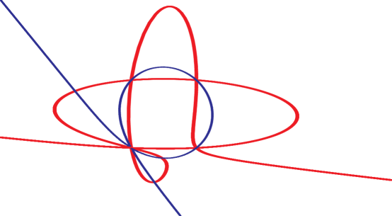
Figure 1. Degree $3$ adjoint curve of a rational curve of degree $5$

The Gorenstein adjoint ideal has many applications in the geometry of curves.

Example 16.

If $\Gamma$ be an irreducible plane algebraic curve of degree $n$, then $\mathfrak{G}_{n-3}$ cuts out the canonical linear series.

Example 17.

If $\Gamma$ is a rational plane curve of degree $n$, then $\mathfrak{G}_{n-2}$ maps $\Gamma$ to a rational normal curve of degree $n-2$ in $\mathbb{P}^{n-2}$.

Example 18.

The Gorenstein adjoint ideal can be used in the Brill-Noether-Algorithm to compute Riemann-Roch spaces for singular curves.

The Gorenstein adjoint ideal can be computed via a local-to-global strategy.

Definition 19.

The local adjoint ideal of $\Gamma$ at $P\in\operatorname{Sing}\Gamma$ is the largest homogeneous ideal $\mathfrak{G}(P)\subset k[x_{0},\ldots,x_{r}]$ with $\mathfrak{G}(P)_{P}=\mathcal{C}_{\mathcal{O}_{\Gamma,P}}.$

Lemma 20.

[5, Prop. 5.4] With notation as above,

$$\mathfrak{G}={\bigcap\nolimits_{P\in\operatorname{Sing}\Gamma}}\mathfrak{G}(P).$$

Definition 21.

Let $A$ be the coordinate ring of an affine model $C=\operatorname{Spec}A$ of $\Gamma$ and let $P\in\operatorname{Sing}(A)$. A ring $A\subset B\subset\overline{A}\subset\operatorname{Quot}(A)$ is called a minimal local contribution to $\overline{A}$ at $P$ if $B_{P}=\overline{A_{P}}$ and $B_{Q}=A_{Q}$ for all $P\neq Q\in C$.

The minimal local contribution to $\overline{A}$ at $P$ is unique and can be computed using Grauert-Remmert-type normalization algorithms, see [4]. It can be written as $B=\frac{U}{d}$ with an ideal $U\subset A$ and a common denominator $d\in A$.

Algorithm 22.

[5, Alg. 4] With notation as above, $\mathfrak{G}(P)\subset k[x_{0},\ldots,x_{r}]$ is the homogenization of the preimage of $\left(d:U\right)$ under $k[x_{1},\ldots,x_{r}]\rightarrow k[x_{1},\ldots,x_{r}]/I=A$.

7. Modular version of the algorithm

Applying the general modular strategy gives an algorithm which is two-fold parallel (taking Lemma 20 into account). We use primes $p$ such that the algorithm is applicable to the variety $\Gamma_{p}$ defined by $I(\Gamma)_{p}$. Efficient verification can be realized through a semi-continuity argument, see [5, Theorem 8.14]. Table 1 gives timings (in seconds on a 2.2 GHz processor) for plane curves $f_{n}$ of degree $n$ with $\binom{n-1}{2}$ singularities of type $A_{1}$.

Rows LA and IQ refer to global computations of the Gorenstein adjoint ideal via linear algebra [9] and ideal quotients, respectively. The row Maple-IB shows timings for the normalization of the curve via a computation of an integral basis in Maple [10]. The row locIQ gives timings for the local-to-global (Lemma 20), and modLocIQ for the modular local-to-global strategy. We also give timings for parallel computations and for the modular probabilistic algorithm obtained by omitting the verification. In square brackets, the number of primes in the modular strategy is shown, in round brackets the number of cores used simultaneously in a parallel computation.

	parallel	probabilistic	$f_{5}$		$f_{6}$		$f_{7}$
Maple-IB			5.1		47		318
LA			98		4400		-
IQ			1.3		54		3800
locIQ	$\blacksquare$		1.3	(1)	54	(1)	3800	(1)
modLocIQ			6.4	[33]	19	[53]	150	[75]
		$\blacksquare$	6.2	[33]	18	[53]	104	[75]
	$\blacksquare$		.36	(74)	1.6	(153)	51	(230)
	$\blacksquare$	$\blacksquare$	.21	(74)	0.48	(153)	5.2	(230)

Table 1. Timings

Observe that, in the example, a local-to-global strategy does not give any benefit when computing over the rationals, since the singular locus does not decompose. However, by Chebotarev’s density theorem, the singular locus is likely to decompose when passing to a finite field, as illustrated by the last two rows of the table.

References

- [1] Arbarello, E.; Ciliberto, C.: Adjoint hypersurfaces to curves in following Petri, in Commutative Algebra, Lecture Notes in Pure and Applied Mathematics, vol. 84, Dekker, New York, 1-21 (1983).
- [2] Arnold, E. A.: Modular algorithms for computing Gröbner bases, J. Symb. Comput. 35, 403–419 (2003).
- [3] J. Böhm, W. Decker, C. Fieker, G. Pfister. The use of bad primes in rational reconstruction, Math. Comp. 84, 3013–3027 (2015).
- [4] J. Böhm, W. Decker, S. Laplagne, G. Pfister, A. Steenpaß, S. Steidel. Parallel algorithms for normalization, J. Symb. Comp. 51, 99–114 (2013).
- [5] J. Böhm, W. Decker, G. Pfister, S. Laplagne. Local to global algorithms for the Gorenstein adjoint ideal of a curve, Preprint (2015), arXiv:1505.05040.
- [6] Decker, W., Greuel, G.-M., Pfister, G., Schönemann, H., 2015. Singular 4-0-2 – A computer algebra system for polynomial computations. http://www.singular.uni-kl.de
- [7] G.-M. Greuel, S. Laplagne, S. Seelisch, Normalization of rings, J. Symb. Comp. 45(9), 887–901 (2010).
- [8] P. Kornerup, R. T. Gregory, Mapping integers and Hensel codes onto Farey fractions, BIT 23, 9–20 (1983).
- [9] Mnuk, M.: An algebraic approach to computing adjoint curves. J. Symbolic Comput., 23(2-3), 229-240 (1997).
- [10] van Hoeij, M.: An algorithm for computing an integral basis in an algebraic function field. J. Symbolic Comput. 18, no. 4, 353-363 (1994).