Analyzing New Physics in $\bar{B}^{0}\to D^{(\ast)}\tau^{-}\bar{\nu}_{\tau}$

Abstract

We discuss possible new physics (NP) effects beyond the standard model (SM) in the exclusive decays $\bar{B}^{0}\to D^{(\ast)}\tau^{-}\bar{\nu}_{\tau}$. Starting with a model-independent effective Hamiltonian including non-SM four-Fermi operators, we show how to obtain experimental constraints on different NP scenarios and investigate their effects on a large set of physical observables. The $\bar{B}^{0}\to D^{(\ast)}$ transition form factors are calculated in the full kinematic $q^{2}$ range by employing the covariant confined quark model developed by our group.

1 Introduction

The exclusive semileptonic decays $\bar{B}^{0}\to D^{(\ast)}\tau^{-}\bar{\nu}_{\tau}$ have been measured by the BABAR [1], Belle [2], and LHCb [3] collaborations in an effort to unravel the well-known $R_{D^{(*)}}$ puzzle which has persisted for several years (see [4, 5, 6] and references therein). The current world averages of the ratios are $R_{D}=0.406\pm 0.050$ and $R_{D^{\ast}}=0.311\pm 0.016$, which exceed the SM predictions of $R_{D}=0.300\pm 0.008$ [7] and $R_{D^{\ast}}=0.252\pm 0.003$ [8] by $2.1\sigma$ and $3.6\sigma$, respectively.

The excess of $R(D^{(\ast)})$ over SM predictions has attracted a great deal of attention in the particle physics community and has led to many theoretical studies looking for NP explanations. Some studies focus on specific NP models including two-Higgs-doublet models [9], leptoquark models [10], and other extensions of the SM. Other studies adopt a model-independent approach, in which a general effective Hamiltonian for the $b\to c\ell\nu$ transition in the presence of NP is imposed to investigate the impact of various NP operators on different physical observables [11]. Most of the theoretical studies rely on the heavy quark effective theory (HQET) [12] to evaluate the hadronic form factors, which are expressed through a few universal functions in the heavy quark limit (HQL). In the present analysis, we employ an alternative approach to calculate the NP-induced hadronic transitions based on the covariant confined quark model (CCQM), which has been developed in some earlier papers by us (see [13] and references therein).

Here we follow the authors of [11] to include NP operators in the effective Hamiltonian and investigate their effects on physical observables of the decays $\bar{B}^{0}\to D^{(\ast)}\ell^{-}\bar{\nu}_{\ell}$. We define a full set of form factors corresponding to SM+NP operators and calculate them by employing the CCQM. In the CCQM the transition form factors can be determined in the full range of momentum transfer, making the calculations straightforward without any extrapolation. This provides an opportunity to investigate NP operators in a self-consistent manner, and independently from the HQET. We first constrain the NP operators using experimental data on the ratios of branching fractions, then analyze their effects on various observables. We also derive the fourfold angular distribution for the cascade decay $\bar{B}^{0}\to D^{\ast\,+}(\to D^{0}\pi^{+})\tau^{-}\bar{\nu}_{\tau}$ to analyze the polarization of the $D^{\ast}$ meson in the presence of NP.

2 Effective operators and helicity amplitudes

Assuming that all neutrinos are left-handed and that NP effects only influence leptons of the third generation, the effective Hamiltonian for the quark-level transition $b\to c\tau^{-}\bar{\nu}_{\tau}$ is given by

$${\mathcal{H}}_{eff} = \frac{4G_{F}}{\sqrt{2}}V_{cb}\left[\mathcal{O}_{V_{L}}+\sum\limits_{X=S_{L},S_{R},V_{L},V_{R},T_{L}}X\mathcal{O}_{X}\right],$$

where the four-Fermi operators $\mathcal{O}_{X}$ are defined as $(i=L,R)$

$$\mathcal{O}_{V_{i}} = \left(\bar{c}\gamma^{\mu}P_{i}b\right)\left(\bar{\tau}\gamma_{\mu}P_{L}\nu_{\tau}\right),$$

$$\mathcal{O}_{S_{i}} = \left(\bar{c}P_{i}b\right)\left(\bar{\tau}P_{L}\nu_{\tau}\right),$$

$$\mathcal{O}_{T_{L}} = \left(\bar{c}\sigma^{\mu\nu}P_{L}b\right)\left(\bar{\tau}\sigma_{\mu\nu}P_{L}\nu_{\tau}\right).$$

Here, $\sigma_{\mu\nu}=i\left[\gamma_{\mu},\gamma_{\nu}\right]/2$, $P_{L,R}=(1\mp\gamma_{5})/2$ are the left and right projection operators, and $X$’s are the complex Wilson coefficients governing the NP contributions, which are equal to zero in the SM.

The invariant form factors describing the hadronic transitions $\bar{B}^{0}\to D$ and $\bar{B}^{0}\to D^{\ast}$ are defined as follows:

$$\langle D(p_{2})|\bar{c}\gamma^{\mu}b|\bar{B}^{0}(p_{1})\rangle = F_{+}(q^{2})P^{\mu}+F_{-}(q^{2})q^{\mu},$$

$$\langle D(p_{2})|\bar{c}b|\bar{B}^{0}(p_{1})\rangle = (m_{1}+m_{2})F^{S}(q^{2}),$$

$$\langle D(p_{2})|\bar{c}\sigma^{\mu\nu}(1-\gamma^{5})b|\bar{B}^{0}(p_{1})\rangle = \frac{iF^{T}(q^{2})}{m_{1}+m_{2}}\left(P^{\mu}q^{\nu}-P^{\nu}q^{\mu}+i\varepsilon^{\mu\nu Pq}\right),$$

$$\langle D^{\ast}(p_{2})|\bar{c}\gamma^{\mu}(1\mp\gamma^{5})b|\bar{B}^{0}(p_{1})\rangle = \frac{\epsilon^{\dagger}_{2\alpha}}{m_{1}+m_{2}}\Big{[}\mp g^{\mu\alpha}PqA_{0}(q^{2})\pm P^{\mu}P^{\alpha}A_{+}(q^{2})$$

$$\pm q^{\mu}P^{\alpha}A_{-}(q^{2})+i\varepsilon^{\mu\alpha Pq}V(q^{2})\Big{]},$$

$$\langle D^{\ast}(p_{2})|\bar{c}\gamma^{5}b|\bar{B}^{0}(p_{1})\rangle = \epsilon^{\dagger}_{2\alpha}P^{\alpha}G^{S}(q^{2}),$$

$$\langle D^{\ast}(p_{2})|\bar{c}\sigma^{\mu\nu}(1-\gamma^{5})b|\bar{B}^{0}(p_{1})\rangle = -i\epsilon^{\dagger}_{2\alpha}\Big{[}\left(P^{\mu}g^{\nu\alpha}-P^{\nu}g^{\mu\alpha}+i\varepsilon^{P\mu\nu\alpha}\right)G_{1}^{T}(q^{2})$$

$$+\left(q^{\mu}g^{\nu\alpha}-q^{\nu}g^{\mu\alpha}+i\varepsilon^{q\mu\nu\alpha}\right)G_{2}^{T}(q^{2})$$

$$+\left(P^{\mu}q^{\nu}-P^{\nu}q^{\mu}+i\varepsilon^{Pq\mu\nu}\right)P^{\alpha}\frac{G_{0}^{T}(q^{2})}{(m_{1}+m_{2})^{2}}\Big{]},$$

where $P=p_{1}+p_{2}$, $q=p_{1}-p_{2}$, and $\epsilon_{2}$ is the polarization vector of the $D^{\ast}$ meson which satisfies the condition $\epsilon_{2}^{\dagger}\cdot p_{2}=0$. The particles are on their mass shells: $p_{1}^{2}=m_{1}^{2}=m_{\bar{B}^{0}}^{2}$ and $p_{2}^{2}=m_{2}^{2}=m_{D^{(\ast)}}^{2}$.

Using the helicity technique first described in [14] and further discussed in our recent papers [4, 5], one obtains the ratio of branching fractions $R_{D^{(*)}}(q^{2})$ as follows:

$$R_{D^{(*)}}(q^{2})=\left(\frac{q^{2}-m_{\tau}^{2}}{q^{2}-m_{\mu}^{2}}\right)^{2}\frac{{\cal H}_{tot}^{D^{(\ast)}}}{\sum\limits_{n}|H_{n}|^{2}+\delta_{\mu}\big{(}\sum\limits_{n}|H_{n}|^{2}+3|H_{t}|^{2}\big{)}},$$

$${\cal H}_{tot}^{D} = |1+g_{V}|^{2}\left[|H_{0}|^{2}+\delta_{\tau}(|H_{0}|^{2}+3|H_{t}|^{2})\right]+\frac{3}{2}|g_{S}|^{2}|H_{P}^{S}|^{2}$$

$$+3\sqrt{2\delta_{\tau}}{\rm Re}g_{S}H_{P}^{S}H_{t}+8|T_{L}|^{2}(1+4\delta_{\tau})|H_{T}|^{2}+12\sqrt{2\delta_{\tau}}{\rm Re}T_{L}H_{0}H_{T},$$

$${\cal H}_{tot}^{D^{\ast}} = (|1+V_{L}|^{2}+|V_{R}|^{2})\Big{[}\sum\limits_{n}|H_{n}|^{2}+\delta_{\tau}\Big{(}\sum\limits_{n}|H_{n}|^{2}+3|H_{t}|^{2}\Big{)}\Big{]}+\frac{3}{2}|g_{P}|^{2}|H^{S}_{V}|^{2}$$

$$-2{\rm Re}V_{R}\big{[}(1+\delta_{\tau})(|H_{0}|^{2}+2H_{+}H_{-})+3\delta_{\tau}|H_{t}|^{2}\big{]}-3\sqrt{2\delta_{\tau}}{\rm Re}g_{P}H^{S}_{V}H_{t}$$

$$+8|T_{L}|^{2}(1+4\delta_{\tau})\sum\limits_{n}|H_{T}^{n}|^{2}-12\sqrt{2\delta_{\tau}}{\rm Re}T_{L}\sum\limits_{n}H_{n}H_{T}^{n}.$$

Here, $\delta_{\ell}=m^{2}_{\ell}/2q^{2}$ is the helicity flip factor, $g_{V}\equiv V_{L}+V_{R}$, $g_{S}\equiv S_{L}+S_{R}$, $g_{P}\equiv S_{L}-S_{R}$, and the index $n$ runs through $(0,+,-)$. The definition of the hadronic helicity amplitudes $H$ in terms of the invariant form factors is presented in the Appendix of [6]. Note that we do not consider interference terms between different NP operators since we assume the dominance of only one NP operator besides the SM contribution.

3 Form factors in the CCQM

As has been discussed in detail in [5] we calculate the current-induced $B\to D^{(\ast)}$ transitions from their one-loop quark diagrams. As a result the various form factors in our model are represented by threefold integrals which are calculated by using fortran codes in the full kinematical momentum transfer region $0\leq q^{2}\leq q^{2}_{max}=(m_{\bar{B}^{0}}-m_{D^{(\ast)}})^{2}$. Our numerical results for the form factors are well represented by a double-pole parametrization

$$F(q^{2})=\frac{F(0)}{1-as+bs^{2}},\quad s=\frac{q^{2}}{m_{1}^{2}}.$$

The parameters of the form factors for the $\bar{B}^{0}\to D$ and $\bar{B}^{0}\to D^{\ast}$ transitions are listed in Table 1.

	$\bar{B}^{0}\to D^{\ast}$								$\bar{B}^{0}\to D$
	$A_{0}$	$A_{+}$	$A_{-}$	$V$	$G^{S}$	$G_{0}^{T}$	$G_{1}^{T}$	$G_{2}^{T}$	$F_{+}$	$F_{-}$	$F^{S}$	$F^{T}$
$F(0)$	1.62	0.67	$-0.77$	0.77	$-0.50$	$-0.073$	0.73	$-0.37$	0.79	$-0.36$	0.80	0.77
$a$	0.34	0.87	0.89	0.90	0.87	1.23	0.90	0.88	0.75	0.77	0.22	0.76
$b$	$-0.16$	0.057	0.070	0.075	0.060	0.33	0.074	0.065	0.039	0.046	$-0.098$	0.043
$F(q^{2}_{\rm max})$	1.91	0.99	$-1.15$	1.15	$-0.74$	$-0.13$	1.10	$-0.55$	1.14	$-0.53$	0.89	1.11
$F^{HQL}(q^{2}_{\rm max})$	1.99	1.12	$-1.12$	1.12	$-0.62$	0	1.12	$-0.50$	1.14	$-0.54$	0.88	1.14

Table 1: Parameters of the dipole approximation for $\bar{B}^{0}\to D^{(\ast)}$ form factors. Zero-recoil values of the form factors are also listed for comparison with the HQET.

We also list the zero-recoil values of the form factors for comparison with the corresponding HQET results which can e.g. be found in [5]. The agreement between the two sets of zero-recoil values is within $10\%$. It is worth mentioning that we obtain a nonzero result for the form factor $G_{0}^{T}$ at zero recoil, which is predicted to vanish in the HQET.

We note that in [4] the HQL in our approach was explored in great detail for the heavy-to-heavy $\bar{B}^{0}\to D^{(\ast)}$ transitions. In [4] we also calculated the Isgur-Wise function and considered the near-recoil behavior of the form factors. A brief discussion of the subleading corrections to the HQL arising from finite quark masses can be found in Appendix B of [5]. Finally, we briefly discuss some error estimates within our model. We fix our model parameters (the constituent quark masses, the infrared cutoff, and the hadron size parameters) by minimizing the functional $\chi^{2}=\sum\limits_{i}\frac{(y_{i}^{\rm expt}-y_{i}^{\rm theor})^{2}}{\sigma^{2}_{i}}$ where $\sigma_{i}$ is the experimental uncertainty. If $\sigma$ is too small then we take its value of 10$\%$. Moreover, we observed that the errors of the fitted parameters are of the order of 10$\%$. Thus we estimate the model uncertainties to lie within 10$\%$.

4 Experimental constraints

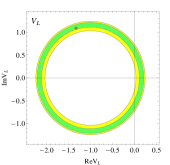
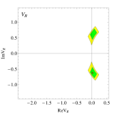
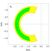
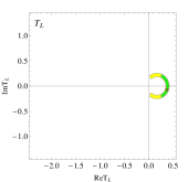
Figure 1: Constraints on the Wilson coefficients $V_{L}$, $V_{R}$, $S_{L}$, and $T_{L}$ within $1\sigma$ (green, dark) and $2\sigma$ (yellow, light). No value of $S_{R}$ is allowed within $2\sigma$. The best-fit value in each case is denoted with the symbol $\ast$.

Within the SM (without any NP operators) our model calculation yields $R(D)=0.267$ and $R(D^{\ast})=0.238$, which are consistent with other SM predictions given in [7, 8] within $10\%$.

Assuming the dominance of only one NP operator at a time (besides the SM one), we compare the calculated ratios $R_{D^{(\ast)}}$ with the current experimental data $R_{D}=0.406\pm 0.050$ and $R_{D^{\ast}}=0.311\pm 0.016$ and obtain the allowed regions for the NP couplings as shown in Fig. 1.

It is important to note that while determining these regions, we also take into account a theoretical error of $10\%$ for the ratios $R(D^{(\ast)})$. The vector operators $\mathcal{O}_{V_{L,R}}$ and the left scalar operator $\mathcal{O}_{S_{L}}$ are favored while there is no allowed region for the right scalar operator $\mathcal{O}_{S_{R}}$ within $2\sigma$. Therefore we will not consider $\mathcal{O}_{S_{R}}$ in what follows. The tensor operator $\mathcal{O}_{T_{L}}$ is less favored, but it can still well explain the current experimental results. In each allowed region at $2\sigma$ we find the best-fit value for each NP coupling. The best-fit couplings read $V_{L}=-1.33+i1.11$, $V_{R}=0.03-i0.60$, $S_{L}=-1.79-i0.22$, $T_{L}=0.38-i0.06$, and are marked with an asterisk.

5 The cascade decay $\bar{B}^{0}\to D^{\ast+}(\to D^{0}\pi^{+})\tau^{-}\bar{\nu}_{\tau}$ and the
angular observables

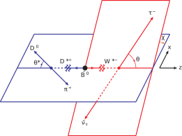
Figure 2: Definition of the angles $\theta$, $\theta^{\ast}$ and $\chi$ in the cascade decay $\bar{B}^{0}\to D^{\ast+}(\to D^{0}\pi^{+})\tau^{-}\bar{\nu}_{\tau}$.

5.1 The fourfold distribution

In order to analyze NP effects on the polarization of the $D^{\ast}$ meson one uses the cascade decay $\bar{B}^{0}\to D^{\ast+}(\to D^{0}\pi^{+})\tau^{-}\bar{\nu}_{\tau}$. A detailed derivation of the fourfold angular distribution (without NP) can be found in our paper [15]. The three angles $\theta$, $\theta^{\ast}$, and $\chi$ in the distribution are defined in Fig. 2 One has

$$\frac{d^{4}\Gamma(\bar{B}^{0}\to D^{\ast+}(\to D^{0}\pi^{+})\tau^{-}\bar{\nu}_{\tau})}{dq^{2}d\cos\theta d\chi d\cos\theta^{\ast}}$$

$$=\frac{9}{8\pi}|N|^{2}J(\theta,\theta^{\ast},\chi),$$

where

$$|N|^{2}=\frac{G_{F}^{2}|V_{cb}|^{2}|{\bf p_{2}}|q^{2}v^{2}}{(2\pi)^{3}12m_{1}^{2}}\mathcal{B}(D^{\ast}\to D\pi).$$

The full angular distribution $J(\theta,\theta^{\ast},\chi)$ is written as

$$J(\theta,\theta^{\ast},\chi)$$

$$= J_{1s}\sin^{2}\theta^{\ast}+J_{1c}\cos^{2}\theta^{\ast}+(J_{2s}\sin^{2}\theta^{\ast}+J_{2c}\cos^{2}\theta^{\ast})\cos 2\theta$$

$$+J_{3}\sin^{2}\theta^{\ast}\sin^{2}\theta\cos 2\chi+J_{4}\sin 2\theta^{\ast}\sin 2\theta\cos\chi$$

$$+J_{5}\sin 2\theta^{\ast}\sin\theta\cos\chi+(J_{6s}\sin^{2}\theta^{\ast}+J_{6c}\cos^{2}\theta^{\ast})\cos\theta$$

$$+J_{7}\sin 2\theta^{\ast}\sin\theta\sin\chi+J_{8}\sin 2\theta^{\ast}\sin 2\theta\sin\chi+J_{9}\sin^{2}\theta^{\ast}\sin^{2}\theta\sin 2\chi,$$

where $J_{i(a)}$ $(i=1,\dots,9;a=s,c)$ are the angular observables. Their explicit expressions in terms of helicity amplitudes and Wilson coefficients can be found in our paper [5]. The fourfold distribution allows one to define a large set of observables which can help probe NP in the decay. First, by integrating the angular decay distribution over all angles one obtains

$$\frac{d\Gamma(\bar{B}^{0}\to D^{\ast}\tau^{-}\bar{\nu}_{\tau})}{dq^{2}}=|N|^{2}J_{\rm tot}=|N|^{2}(J_{L}+J_{T}),$$

where $J_{L}=3J_{1c}-J_{2c}$ and $J_{T}=2(3J_{1s}-J_{2s})$ are the longitudinal and transverse polarization amplitudes of the $D^{\ast}$ meson. In Fig. 3 we present the $q^{2}$ dependence of the rate ratios $R_{D^{(\ast)}}(q^{2})$ in different NP scenarios. It is interesting to note that unlike the vector and scalar operators, which tend to increase both ratios, the tensor operator can lead to a decrease of the ratio $R(D^{\ast})$ for $q^{2}\gtrsim 8~{}\text{GeV}^{2}$. Moreover, while the ratio $R(D^{\ast})$ is minimally sensitive to the scalar coupling $S_{L}$ (in comparison with other couplings, i.e. $V_{L,R}$, $T_{L}$), the ratio $R(D)$ shows maximal sensitivity to $S_{L}$. These behaviors can help discriminate between different NP operators.

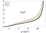
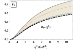
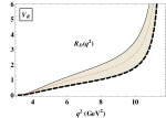
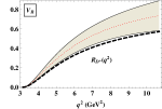
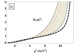
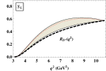
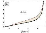
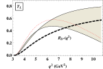
Figure 3: $R_{D}(q^{2})$ (left) and $R_{D^{\ast}}(q^{2})$ (right). The thick black dashed lines are the SM prediction; the gray bands include NP effects corresponding to the $2\sigma$ allowed regions in Fig. 1; the red dotted lines represent the best-fit values.

5.2 The $\cos\theta$ distribution, the forward-backward asymmetry, and the lepton-side convexity parameter

We define a normalized angular decay distribution $\widetilde{J}(\theta^{\ast},\theta,\chi)$ through

$$\widetilde{J}(\theta^{\ast},\theta,\chi)=\frac{9}{8\pi}\frac{J(\theta^{\ast},\theta,\chi)}{J_{\rm tot}},$$

where $J_{\rm tot}=3J_{1c}+6J_{1s}-J_{2c}-2J_{2s}$. The normalized angular decay distribution $\widetilde{J}(\theta^{\ast},\theta,\chi)$ obviously integrates to $1$ after $\cos\theta^{\ast},\,\cos\theta$, and $\chi$ integration. By integrating the fourfold distribution over $\cos\theta^{\ast}$ and $\chi$ one obtains the differential $\cos\theta$ distribution which is described by a tilted parabola. The normalized form of the parabola reads

$$\widetilde{J}(\theta)=\frac{a+b\cos\theta+c\cos^{2}\theta}{2(a+c/3)}.$$

The linear coefficient $b/2(a+c/3)$ can be projected out by defining a forward-backward asymmetry given by

$$\mathcal{A}_{FB}(q^{2})$$

$$=\frac{[\int_{0}^{1}-\int_{-1}^{0}]d\cos\theta\,d\Gamma/d\cos\theta}{[\int_{0}^{1}+\int_{-1}^{0}]d\cos\theta\,d\Gamma/d\cos\theta}$$

$$=\frac{b}{2(a+c/3)}=\frac{3}{2}\frac{J_{6c}+2J_{6s}}{J_{\rm tot}}.$$

The coefficient $c/2(a+c/3)$ of the quadratic contribution is obtained by taking the second derivative of $\widetilde{J}(\theta)$. Accordingly, we define a convexity parameter by writing

$$C_{F}^{\tau}(q^{2})=\frac{d^{2}\widetilde{J}(\theta)}{d(\cos\theta)^{2}}=\frac{c}{a+c/3}=\frac{6(J_{2c}+2J_{2s})}{J_{\rm tot}}.$$

The $q^{2}$ dependence of $\mathcal{A}_{FB}$ is shown in Fig. 4. The coupling $V_{L}$ does not effect $\mathcal{A}_{FB}$ in both decays. In the case of the $\bar{B}^{0}\to D^{\ast}$ transition, the operators $\mathcal{O}_{V_{R}}$, $\mathcal{O}_{S_{L}}$, and $\mathcal{O}_{T_{L}}$ behave mostly similarly: they tend to decrease $\mathcal{A}_{FB}$ and shift the zero-crossing point to greater values than the SM one. However, the tensor operator can also increase $\mathcal{A}_{FB}$ in the high-$q^{2}$ region. In the case of the $\bar{B}^{0}\to D$ transition, the operator $\mathcal{O}_{V_{R}}$ does not affect $\mathcal{A}_{FB}$, the tensor operator $\mathcal{O}_{T_{L}}$ tends to lower $\mathcal{A}_{FB}$, and the scalar operator $\mathcal{O}_{S_{L}}$ thoroughly changes $\mathcal{A}_{FB}$: it can increase $\mathcal{A}_{FB}$ by up to $200\%$ and implies a zero-crossing point, which is impossible in the SM. This unique effect of $\mathcal{O}_{S_{L}}$ would clearly distinguish it from the other NP operators.

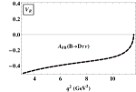
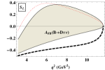
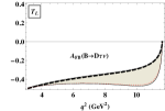
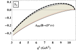
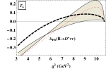
Figure 4: Forward-backward asymmetry $\mathcal{A}_{FB}$ for $\bar{B}^{0}\to D\tau^{-}\bar{\nu}_{\tau}$ (upper) and $\bar{B}^{0}\to D^{\ast}\tau^{-}\bar{\nu}_{\tau}$ (lower). Notations are the same as in Fig. 3.

In Fig. 5 we present the lepton-side convexity parameter $C_{F}^{\tau}(q^{2})$.

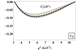
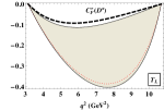
Figure 5: Lepton-side convexity parameter $C_{F}^{\tau}(q^{2})$.

While $C_{F}^{\tau}(D)$ is only sensitive to $\mathcal{O}_{T_{L}}$, $C_{F}^{\tau}(D^{\ast})$ is sensitive to $\mathcal{O}_{S_{L}}$, $\mathcal{O}_{V_{R}}$, and $\mathcal{O}_{T_{L}}$. Unlike $\mathcal{O}_{S_{L}}$, which can only increase $C_{F}^{\tau}(D^{\ast})$, the operator $\mathcal{O}_{T_{L}}$ can only lower the parameter. It is worth mentioning that $C_{F}^{\tau}(D)$ and $C_{F}^{\tau}(D^{\ast})$ are extremely sensitive to $\mathcal{O}_{T_{L}}$: it can change $C_{F}^{\tau}(D^{(\ast)})$ by a factor of 4 at $q^{2}\approx 7~{}\text{GeV}^{2}$.

5.3 The $\cos\theta^{\ast}$ distribution and the hadron-side convexity parameter

By integrating the fourfold distribution over $\cos\theta$ and $\chi$ one obtains the hadron-side $\cos\theta^{\ast}$ distribution described by an untilted parabola (without a linear term). The normalized form of the $\cos\theta^{\ast}$ distribution reads $\widetilde{J}(\theta^{\ast})=(a^{\prime}+c^{\prime}\cos^{2}\theta^{\ast})/2(a^{\prime}+c^{\prime}/3)$, which can again be characterized by its convexity parameter given by

$$C_{F}^{h}(q^{2})=\frac{d^{2}\widetilde{J}(\theta^{\ast})}{d(\cos\theta^{\ast})^{2}}=\frac{c^{\prime}}{a^{\prime}+c^{\prime}/3}=\frac{3J_{1c}-J_{2c}-3J_{1s}+J_{2s}}{J_{\rm tot}/3}.$$

The $\cos\theta^{\ast}$ distribution can be written as

$$\widetilde{J}(\theta^{\ast})=3/4\cdot\left(2F_{L}(q^{2})\cos^{2}\theta^{\ast}+F_{T}(q^{2})\sin^{2}\theta^{\ast}\right),$$

where $F_{L}(q^{2})$ and $F_{T}(q^{2})$ are the polarization fractions of the $D^{\ast}$ meson and are defined as

$$F_{L}(q^{2})=J_{L}/(J_{L}+J_{T}),\qquad F_{T}(q^{2})=J_{T}/(J_{L}+J_{T}),\qquad F_{L}(q^{2})+F_{T}(q^{2})=1.$$

The hadron-side convexity parameter and the polarization fractions of the $D^{\ast}$ are related by

$$C_{F}^{h}(q^{2})=3/2\cdot\left(2F_{L}(q^{2})-F_{T}(q^{2})\right)=3/2\cdot\left(3F_{L}(q^{2})-1\right).$$

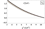
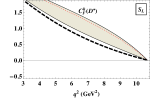
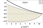
Figure 6: Hadron-side convexity parameter $C_{F}^{h}(q^{2})$. Notations are the same as in Fig. 3.

The effects of NP operators on the hadron-side convexity parameter $C_{F}^{h}(q^{2})$ are shown in Fig. 6. Each NP operator can change $C_{F}^{h}(q^{2})$ in a unique way: the vector operator $\mathcal{O}_{V_{R}}$ almost does nothing to the parameter; the scalar operator $\mathcal{O}_{S_{L}}$ increases the parameter by about $50\%$ nearly in the whole range of $q^{2}$; the tensor operator $\mathcal{O}_{T_{L}}$ lowers the parameter (by up to $200\%$ at low $q^{2}$), and it also allows negative values of $C_{F}^{h}(q^{2})$, which are impossible in the SM.

5.4 The $\chi$ distribution and the trigonometric moments

By integrating the fourfold distribution over $\cos\theta$ and $\cos\theta^{\ast}$, one obtains the $\chi$ distribution whose normalized form reads

$$\widetilde{J}^{(I)}(\chi)=\Big{[}1+A_{C}^{(1)}(q^{2})\cos 2\chi+A_{T}^{(1)}(q^{2})\sin 2\chi\Big{]}/(2\pi),$$

where $A_{C}^{(1)}(q^{2})=4J_{3}/J_{\rm tot}$ and $A_{T}^{(1)}(q^{2})=4J_{9}/J_{\rm tot}$. Besides, one can also define other angular distributions in the angular variable $\chi$ as follows:

$$J^{(II)}(\chi) = \Big{[}\int_{0}^{1}-\int_{-1}^{0}\Big{]}d\cos\theta^{\ast}\int_{-1}^{1}d\cos\theta\frac{d^{4}\Gamma}{dq^{2}d\cos\theta d\chi d\cos\theta^{\ast}},$$

$$J^{(III)}(\chi) = \Big{[}\int_{0}^{1}-\int_{-1}^{0}\Big{]}d\cos\theta^{\ast}\Big{[}\int_{0}^{1}-\int_{-1}^{0}\Big{]}d\cos\theta\frac{d^{4}\Gamma}{dq^{2}d\cos\theta d\chi d\cos\theta^{\ast}}.$$

The normalized forms of these distributions read

$$\widetilde{J}^{(II)}(\chi) = \frac{1}{4}\Big{[}A_{C}^{(2)}(q^{2})\cos\chi+A_{T}^{(2)}(q^{2})\sin\chi\Big{]},$$

$$\widetilde{J}^{(III)}(\chi) = \frac{2}{3\pi}\Big{[}A_{C}^{(3)}(q^{2})\cos\chi+A_{T}^{(3)}(q^{2})\sin\chi\Big{]},$$

where $A_{C}^{(2)}(q^{2})=3J_{5}/J_{\rm tot},\quad A_{T}^{(2)}(q^{2})=3J_{7}/J_{\rm tot},\quad A_{C}^{(3)}(q^{2})=3J_{4}/J_{\rm tot},\quad A_{T}^{(3)}(q^{2})=3J_{8}/J_{\rm tot}$.

Another method to project the coefficient functions $J_{i}$ $(i=3,4,5,7,8,9)$ out from the fourfold angular decay distribution is to take the appropriate trigonometric moments of the normalized decay distribution $\widetilde{J}(\theta^{\ast},\theta,\chi)$ [4]. The trigonometric moments are defined by

$$W_{i}=\int d\cos\theta d\cos\theta^{\ast}d\chi M_{i}(\theta^{\ast},\theta,\chi)\widetilde{J}(\theta^{\ast},\theta,\chi)\equiv\left\langle M_{i}(\theta^{\ast},\theta,\chi)\right\rangle,$$

where $M_{i}(\theta^{\ast},\theta,\chi)$ defines the trigonometric moment that is being taken. One finds

$$W_{T}(q^{2}) \equiv \left\langle\cos 2\chi\right\rangle=2\cdot(J_{3}/J_{\rm tot})=(1/2)\cdot A_{C}^{(1)}(q^{2}),$$

$$W_{IT}(q^{2}) \equiv \left\langle\sin 2\chi\right\rangle=2\cdot(J_{9}/J_{\rm tot})=(1/2)\cdot A_{T}^{(1)}(q^{2}),$$

$$W_{A}(q^{2}) \equiv \left\langle\sin\theta\cos\theta^{\ast}\cos\chi\right\rangle=(3\pi/8)\cdot(J_{5}/J_{\rm tot})=(\pi/8)\cdot A_{C}^{(2)}(q^{2}),$$

$$W_{IA}(q^{2}) \equiv \left\langle\sin\theta\cos\theta^{\ast}\sin\chi\right\rangle=(3\pi/8)\cdot(J_{7}/J_{\rm tot})=(\pi/8)\cdot A_{T}^{(2)}(q^{2}),$$

$$W_{I}(q^{2}) \equiv \left\langle\cos\theta\cos\theta^{\ast}\cos\chi\right\rangle=(9\pi^{2}/128)\cdot(J_{4}/J_{\rm tot})=(3\pi^{2}/128)\cdot A_{C}^{(3)}(q^{2}),$$

$$W_{II}(q^{2}) \equiv \left\langle\cos\theta\cos\theta^{\ast}\sin\chi\right\rangle=(9\pi^{2}/128)\cdot(J_{8}/J_{\rm tot})=(3\pi^{2}/128)\cdot A_{T}^{(3)}(q^{2}).$$

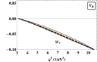
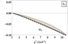
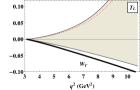
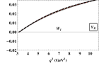
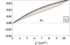
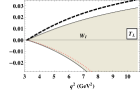
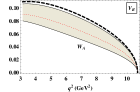
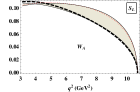
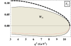
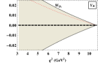
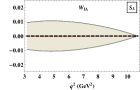
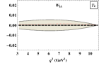
Figure 7: Trigonometric moments $W_{T}(q^{2})$, $W_{I}(q^{2})$, $W_{A}(q^{2})$, and $W_{IA}(q^{2})$. Notations are the same as in Fig. 3.

In Fig. 7 we show the $q^{2}$ dependence of the trigonometric moments $W_{T}(q^{2})$, $W_{I}(q^{2})$, $W_{A}(q^{2})$, and $W_{IA}(q^{2})$. The moments $W_{T}(q^{2})$ and $W_{I}(q^{2})$ are almost insensitive to $\mathcal{O}_{V_{R}}$ but highly sensitive to $\mathcal{O}_{T_{L}}$. The scalar and tensor operators are likely to raise $W_{T}(q^{2})$ and to lower $W_{I}(q^{2})$ in general. The moment $W_{A}(q^{2})$ shows great sensitivity to $\mathcal{O}_{V_{R}}$, $\mathcal{O}_{S_{L}}$, and $\mathcal{O}_{T_{L}}$. Both $\mathcal{O}_{V_{R}}$ and $\mathcal{O}_{T_{L}}$ tend to decrease $W_{A}(q^{2})$ while $\mathcal{O}_{S_{L}}$ tries to do the opposite. It is worth noting that all three moments $W_{T}(q^{2})$, $W_{I}(q^{2})$, and $W_{A}(q^{2})$ are extremely sensitive to $\mathcal{O}_{T_{L}}$ and their sign can change in the presence of $\mathcal{O}_{T_{L}}$. Regarding the moment $W_{IA}(q^{2})$, the three operators act in the same manner: they can change $W_{IA}(q^{2})$ in both directions, and the sensitivity is maximal in the case of $\mathcal{O}_{V_{R}}$.

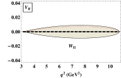
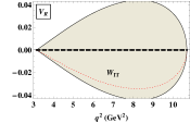
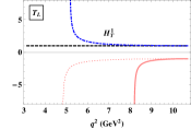
Figure 8: Trigonometric moments $W_{II}(q^{2})$ (left) and $W_{IT}(q^{2})$ (center), and the optimal angular observable $H_{T}^{(1)}(q^{2})$ (right). The black dashed lines are the SM prediction. The red dotted lines represent the best-fit values. The blue dot-dashed line and the pink solid line in the right plot are the predictions for $T_{L}=0.04-0.17i$ and $T_{L}=0.18+0.23i$, respectively.

The trigonometric moments $W_{II}(q^{2})$ and $W_{IT}(q^{2})$ are equal to zero in the SM and obtain a nonzero contribution only from the right-chiral vector operator $\mathcal{O}_{V_{R}}$, as depicted in Fig. 8. Both moments are proportional to the imaginary part of $V_{R}$ and the effect of $\mathcal{O}_{V_{R}}$ cancels in their ratio.

One can also consider certain combinations of angular observables where the form factor dependence drops out (at least in most NP scenarios) [16]. As a demonstration, we consider the optimized observable

$$H_{T}^{(1)}=\sqrt{2}J_{4}/\sqrt{-J_{2c}(2J_{2s}-J_{3})},$$

which is equal to one not only in the SM but also in all NP scenarios except the tensor one, as shown in the right plot of Fig. 8. Therefore $H_{T}^{(1)}(q^{2})$ plays a prominent role in confirming the appearance of the tensor operator $\mathcal{O}_{T_{L}}$ in the decay $\bar{B}^{0}\to D^{\ast}\tau^{-}\bar{\nu}_{\tau}$.

6 Tau polarization as probe for NP

Recently, the Belle collaboration has reported on the first measurement of the longitudinal polarization of the tau lepton in the decay $\bar{B}^{0}\to D^{\ast}\tau^{-}\bar{\nu}_{\tau}$ with the result $P_{L}^{\tau}=-0.38\pm 0.51(\text{stat.})^{+0.21}_{-0.16}(\text{syst.})$ [2]. The errors are quite large but this pioneering measurement has opened a new window on the analysis of the dynamics of the semileptonic $B\to D^{(*)}$ transitions. The hope is that, with the Belle II super-B factory nearing completion, more precise values of the polarization can be achieved in the future, which would shed more light on the search for possible NP in these decays.

In a recent paper [6] we have studied the longitudinal ($P_{L}$), transverse ($P_{T}$), and normal ($P_{N}$) polarization components of the $\tau^{-}$ in $\bar{B}^{0}\to D^{(\ast)}\tau^{-}\bar{\nu}_{\tau}$ and clarified their roles in the search for NP. In [6] one can find the $q^{2}$ dependence of the $\tau^{-}$ polarizations in the presence of NP operators, which bears powerful information for discriminating between different NP scenarios. For example, it can be used to perform a bin-by-bin analysis to probe NP in different $q^{2}$ regions. One can also calculate the average polarizations over the whole $q^{2}$ region. The predictions for the mean polarizations are summarized in Table 2.

$\bar{B}^{0}\to D$
	$<P_{L}^{D}>$	$<P_{T}^{D}>$	$<P_{N}^{D}>$	$<|\vec{P}^{D}|>$
SM (CCQM)	$0.33$	$0.84$	$0$	$0.91$
$S_{L}$	$(0.36,0.67)$	$(-0.68,0.33)$	$(-0.76,0.76)$	$(0.89,0.96)$
$T_{L}$	$(0.13,0.31)$	$(0.78,0.83)$	$(-0.17,0.17)$	$(0.79,0.90)$
$\bar{B}^{0}\to D^{\ast}$
	$<P_{L}^{D^{\ast}}>$	$<P_{T}^{D^{\ast}}>$	$<P_{N}^{D^{\ast}}>$	$<|\vec{P}^{D^{\ast}}|>$
SM (CCQM)	-0.50	0.46	0	0.71
$S_{L}$	$(-0.40,-0.14)$	$(0.47,0.62)$	$(-0.20,0.20)$	$(0.69,0.70)$
$T_{L}$	$(-0.36,0.24)$	$(-0.61,0.26)$	$(-0.17,0.17)$	$(0.23,0.69)$
$V_{R}$	$-0.50$	$(0.32,0.43)$	$0$	$(0.48,0.67)$

Table 2: $q^{2}$ averages of the polarization components and the total polarization. The two rows labeled by SM (CCQM) contain our predictions within the SM with form factors calculated in the CCQM. The predicted intervals for the observables in the presence of NP are given in correspondence with the $2\sigma$ allowed regions of the NP couplings depicted in Fig. 1.

One sees that the $\tau^{-}$ polarization components in $\bar{B}^{0}\to D\tau^{-}\bar{\nu}_{\tau}$ are extremely sensitive to $S_{L}$. When $S_{L}$ is present, $\langle P_{L}^{D}\rangle$ can be as large as $0.67$, $\langle P_{T}^{D}\rangle$ can reach $-0.68$, and $\langle P_{N}^{D}\rangle$ can even reach $\pm 0.76$. It is interesting to note that if one measures $\langle P_{L}^{D}\rangle$ and finds any excess over the SM value, it would be a clear sign of $S_{L}$. Meanwhile, the $\tau^{-}$ longitudinal and transverse polarization components in $\bar{B}^{0}\to D^{\ast}\tau^{-}\bar{\nu}_{\tau}$ are more sensitive to $T_{L}$. The coupling $T_{L}$ can enhance $\langle P_{L}^{D^{\ast}}\rangle$ from the SM value of $-0.50$ up to $0.24$, or lower $\langle P_{T}^{D^{\ast}}\rangle$ from $0.46$ down to $-0.61$. Notably, the average transverse polarization $\langle P_{T}^{D}\rangle$ is almost insensitive to $T_{L}$ in comparison with $S_{L}$. When $T_{L}$ is present, one finds $0.78\leq\langle P_{T}^{D}\rangle\leq 0.83$, which is almost the same as the SM value $\langle P_{T}^{D}\rangle=0.84$. In contrast, if $S_{L}$ is present, one has $-0.68\leq\langle P_{T}^{D}\rangle\leq 0.33$, which is much lower than the SM prediction. This unique property of $\langle P_{T}^{D}\rangle$ may play a very important role in probing the scalar coupling $S_{L}$. It is also interesting to note that the average total polarization $<|\vec{P}^{D^{\ast}}|>$ is almost insensitive to $S_{L}$.

7 Summary and discussion

We have provided a thorough analysis of possible NP in the decays $\bar{B}^{0}\to D^{(\ast)}\tau^{-}\bar{\nu}_{\tau}$ using the form factors obtained from our covariant quark model. Starting with a general effective Hamiltonian including NP operators, we have derived the full angular distribution and defined a large set of physical observables. Assuming NP only affects leptons of the third generation and only one NP operator appears at a time, we have gained the allowed regions of NP couplings based on recent measurements at $B$ factories, and studied their effects on the observables. It has turned out that the current experimental data of $R(D)$ and $R(D^{\ast})$ prefer the operators $\mathcal{O}_{S_{L}}$ and $\mathcal{O}_{V_{L,R}}$, the operator $\mathcal{O}_{T_{L}}$ is less favored, and the operator $\mathcal{O}_{S_{R}}$ is disfavored at $2\sigma$.

Our analysis has been done under the assumption of one-operator dominance. However, the large observable set has revealed unique behaviors of several observables and provided many correlations between them, which allows one to distinguish between NP operators. Our analysis can serve as a map for setting up various strategies to identify the origins of NP, one of which is as follows: first, one uses the null tests $W_{IT}(q^{2})=0$ and $H_{T}^{(1)}(q^{2})-1=0$ to probe the operators $\mathcal{O}_{V_{R}}$ and $\mathcal{O}_{T_{L}}$, respectively. Second, one measures the forward-backward asymmetry in $\bar{B}^{0}\to D\tau^{-}\bar{\nu}_{\tau}$. If $\mathcal{A}_{FB}^{D}(q^{2})$ has a zero-crossing point, then it is a clear sign of $\mathcal{O}_{S_{L}}$. The coupling $V_{L}$ is more difficult to test because it is just a multiplier of the SM operator. However, if the tests above disconfirm $\mathcal{O}_{V_{R}}$, $\mathcal{O}_{T_{L}}$, and $\mathcal{O}_{S_{L}}$ at the same time, then the modification of $V_{L}$ to $R(D)$ and $R(D^{\ast})$ is a must. In the future when more precise data will be collected, one can adopt the strategies described here as a useful tool to discover NP in these decays if the deviation from the SM still remains.

References

- [1] J. Lees et al. (BABAR Collaboration), Phys. Rev. Lett. 109, 101802 (2012).
-
[2]
M. Huschle et al. (Belle Collaboration),
Phys. Rev. D92, 072014 (2015);
Y. Sato et al. (Belle Collaboration), Phys. Rev. D94, 072007 (2016);
S. Hirose et al. (Belle Collaboration), arXiv:1612.00529. - [3] R. Aaij et al. (LHCb Collaboration), Phys. Rev. Lett. 115, 111803 (2015).
- [4] M. A. Ivanov, J. G. Körner, and C. T. Tran, Phys. Rev. D92, 114022 (2015).
- [5] M. A. Ivanov, J. G. Körner and C. T. Tran, Phys. Rev. D94, 094028 (2016).
- [6] M. A. Ivanov, J. G. Körner and C. T. Tran, arXiv:1701.02937 [hep-ph].
- [7] H. Na et al. (HPQCD Collaboration), Phys. Rev. D92, 054510 (2015).
- [8] S. Fajfer, J. F. Kamenik, and I. Nisandzic, Phys. Rev. D85, 094025 (2012).
-
[9]
A. Crivellin, C. Greub and A. Kokulu,
Phys. Rev. D86, 054014 (2012);
A. Celis, M. Jung, X. Q. Li and A. Pich, JHEP 1301, 054 (2013). -
[10]
Y. Sakaki, M. Tanaka, A. Tayduganov and R. Watanabe,
Phys. Rev. D88, 094012 (2013);
M. Bauer and M. Neubert, Phys. Rev. Lett. 116, 141802 (2016);
S. Fajfer and N. Kosnik, Phys. Lett. B755, 270 (2016);
X. Q. Li, Y. D. Yang and X. Zhang, JHEP 1608, 054 (2016). -
[11]
A. Datta, M. Duraisamy and D. Ghosh,
Phys. Rev. D86, 034027 (2012);
D. Becirevic, N. Kosnik and A. Tayduganov, Phys. Lett. B716, 208 (2012);
M. Tanaka and R. Watanabe, Phys. Rev. D87, 034028 (2013);
P. Biancofiore, P. Colangelo and F. De Fazio, Phys. Rev. D87, 074010 (2013);
M. Duraisamy and A. Datta, JHEP 1309, 059 (2013). - [12] M. Neubert, Heavy quark symmetry, Phys. Rept. 245, 259 (1994).
-
[13]
T. Branz et al.,
Phys. Rev. D81, 034010 (2010);
M. A. Ivanov et al. Phys. Rev. D85, 034004 (2012);
M. A. Ivanov and C. T. Tran, Phys. Rev. D92, 074030 (2015). -
[14]
J. G. Körner and G. A. Schuler,
Phys. Lett. B231, 306 (1989);
J. G. Körner and G. A. Schuler, Z. Phys. C 46, 93 (1990). - [15] A. Faessler et al., Eur. Phys. J. direct C 4, 18 (2002).
- [16] T. Feldmann, B. Müller and D. van Dyk, Phys. Rev. D92, 034013 (2015).