Hadronic Vacuum Polarization in QCD
and its Evaluation in the Euclidean

Eduardo de Rafael

Aix-Marseille Université, CNRS, CPT, UMR 7332, 13288 Marseille, France

We discuss a new technique to evaluate integrals of QCD Green’s functions in the Euclidean based on their Mellin-Barnes representation. We present as a first application the evaluation of the lowest order Hadronic Vacuum Polarization (HVP) contribution to the anomalous magnetic moment of the muon $\frac{1}{2}(g_{\mu}-2)_{\mbox{\rm\tiny HVP}}\equiv a_{\mu}^{\rm HVP}$. It is shown that with a precise determination of the slope and curvature of the HVP function at the origin from lattice QCD (LQCD), one can already obtain a result for $a_{\mu}^{\rm HVP}$ which may serve as a test of the determinations based on experimental measurements of the $e^{+}e^{-}$ annihilation cross-section into hadrons.

I Introduction

In this and forthcoming papers we shall be concerned with QCD two-point functions of color singlet local operators with possible insertions of soft operators. These Green’s functions, weighted by appropriate known functions, when integrated over the full range of their Euclidean momenta dependence, govern the hadronic contribution to many electromagnetic and weak interaction processes which appear as low energy observables. Two well known examples, with no soft insertions, are:

1. The Hadronic Vacuum Polarization two-point function:

   $$\Pi_{\mu\nu}(q)=i\int d^{4}x\ e^{iq\cdot x}\langle 0|T\left(J_{\mu}(x)J_{\nu}(0)\right)|0\rangle=(q_{\mu}q_{\nu}-q^{2}g_{\mu\nu})\Pi(Q^{2})\,,\quad Q^{2}=-q^{2}\geq 0\,,$$ (1.1)

   where $J_{\mu}(x)$ denotes the hadronic electromagnetic current in the Standard Model. For the light quarks $u$, $d$, $s$,

   $$J_{\mu}(x)=(-ie)\left\{\frac{2}{3}\bar{u}(x)\gamma^{\mu}u(x)-\frac{1}{3}\bar{d}(x)\gamma^{\mu}d(x)-\frac{1}{3}\bar{s}(x)\gamma^{\mu}s(x)\right\}\,.$$ (1.2)

2. The Left-Right two-point function in the chiral limit:

   $$\Pi_{\rm LR}^{\mu\nu}(q)=2i\int d^{4}x\,e^{iq\cdot x}\langle 0|T\left(L^{\mu}(x)R^{\nu}(0)^{\dagger}\right)|0\rangle=(q^{\mu}q^{\nu}-g^{\mu\nu}q^{2})\Pi_{\rm LR}(Q^{2})\,,\quad Q^{2}=-q^{2}\geq 0\,,$$ (1.3)

   where

   $$L^{\mu}(x)=\bar{d}(x)\gamma^{\mu}\frac{1}{2}(1-\gamma_{5})u(x)\quad\mbox{\rm and}\quad R^{\mu}(x)=\bar{d}(x)\gamma^{\mu}\frac{1}{2}(1+\gamma_{5})u(x)\,.$$ (1.4)

To lowest order in the electromagnetic coupling, the Hadronic Vacuum Polarization (HVP) contribution to the anomalous magnetic moment of the muon $\frac{1}{2}(g_{\mu}-2)_{\mbox{\rm\tiny HVP}}\equiv a_{\mu}^{\rm HVP}$ is governed by a weighted integral [1, 2] of the hadronic photon self-energy function $\Pi(Q^{2})$ in the Euclidean, renormalized on-shell at $Q^{2}=0$:

$$a_{\mu}^{\rm HVP}=\frac{\alpha}{\pi}\int_{0}^{1}dx(1-x)\left[-\Pi\left(Q^{2}\equiv\frac{x^{2}}{1-x}m_{\mu}^{2}\right)\right]\,.$$ (1.5)

This integral requires knowing the function $\Pi(Q^{2})$ all the way from $Q^{2}=0$ ($x=0$) to $Q^{2}=\infty$ ($x=1$). In the second example, the $\pi^{+}-\pi^{0}$ mass difference in the Standard Model, to lowest order in the electroweak coupling and in the chiral limit, is governed by a weighted integral of the function $\Pi_{\rm LR}(Q^{2})$ in the Euclidean over the full range $0\leq Q^{2}\leq\infty$ (see ref. [3] and references therein):

$$(m_{\pi^{+}}^{2}-m_{\pi^{0}}^{2})|_{\rm SM}=\frac{\alpha}{\pi}\frac{3}{4f_{\pi}^{2}}\int_{0}^{\infty}dQ^{2}\left(1-\frac{Q^{2}}{Q^{2}+M_{Z}^{2}}\right)\left(-Q^{2}\Pi_{\rm LR}(Q^{2})\right)\,,$$ (1.6)

The first term in the r.h.s. produces a mass difference of electromagnetic origin [4] while the second one corresponds to the small contribution induced by the electroweak $Z$ gauge boson propagator [3]. Other examples of two-point functions with soft insertions are described e.g. in ref. [5] where references to the relevant literature can also be found.

The purpose of this paper is to describe a new approach to evaluate Euclidean QCD integrals of this type. The problem of computing analytically Green’s functions like $\Pi(Q^{2})$ and $\Pi_{\rm LR}(Q^{2})$ in QCD is due to the fact that QCD perturbation theory (pQCD) is only applicable to short-distances i.e. large $Q^{2}$ values and, in fact, in the case of Green’s functions which are order parameters of spontaneous chiral symmetry breaking, like $\Pi_{\rm LR}(Q^{2})$, pQCD gives no contribution at all in the chiral limit. The Green’s functions in question, however, obey dispersion relations which relate their values in the Euclidean to integrals over spectral functions defined in the Minkowski domain. The hadronic photon self-energy $\Pi(Q^{2})$ above is not an order parameter of spontaneous chiral symmetry breaking and it obeys the subtracted dispersion relation

$$\Pi(Q^{2})=\int_{4m_{\pi^{\pm}}^{2}}^{\infty}\frac{dt}{t}\,\frac{-Q^{2}}{t+Q^{2}}\frac{1}{\pi}\mbox{\rm Im}\Pi(t)\,,$$ (1.7)

while $\Pi_{\rm LR}(Q^{2})$ obeys an unsubtracted dispersion relation

$$\Pi_{\rm LR}(Q^{2})=\int_{m_{\pi^{\pm}}^{2}}^{\infty}dt\frac{1}{t+Q^{2}}\frac{1}{\pi}\mbox{\rm Im}\Pi_{\rm LR}(t)\,.$$ (1.8)

Furthermore, the two spectral functions $\frac{1}{\pi}\mbox{\rm Im}\Pi(t)$ and $\frac{1}{\pi}\mbox{\rm Im}\Pi_{\rm LR}(t)$ are accessible to experiment. The first one is directly accessible to experiment via the one photon $e^{+}e^{-}$ annihilation cross section into hadrons ($m_{e}\rightarrow 0$):

$$\sigma(t)=\frac{4\pi^{2}\alpha}{t}\frac{1}{\pi}\mbox{\rm Im}\Pi(t)\,,$$ (1.9)

and this is in fact the way which $a_{\mu}^{\rm HVP}$ has been evaluated to a high degree of precision [8, 9, 10]. Similarly, the hadronic spectral function $\frac{1}{\pi}\mbox{\rm Im}\Pi_{\rm LR}(t)$, which is the difference:

$$\frac{1}{\pi}\mbox{\rm Im}\Pi_{\rm LR}(t)=\frac{1}{\pi}\mbox{\rm Im}\Pi_{\rm VV}(t)-\frac{1}{\pi}\mbox{\rm Im}\Pi_{\rm AA}(t)$$ (1.10)

of Vector-Vector and Axial-Axial correlation functions, is accessible via $e^{+}e^{-}$ annihilation and hadronic $\tau$-decay data. QCD perturbation theory contributes both to the VV and to the AA correlation functions, but the contribution is the same in the chiral limit and vanishes in the difference.

The two examples above are, however, rather exceptional. In most cases, the associated spectral functions to the Green’s functions one is interested in are not accessible to experimental determination. In that sense, both $\Pi(Q^{2})$ and $\Pi_{\rm LR}(Q^{2})$ provide excellent theoretical laboratories to test non perturbative approaches to the determination of the more general type of Green’s functions we are concerned with.

This first paper is dedicated to the study of the hadronic photon self-energy $\Pi(Q^{2})$ and its contribution to $a_{\mu}^{\rm HVP}$. There is a persistent discrepancy between the latest experimental determination of the anomalous magnetic moment of the muon [6]:

$$a_{\mu}^{\rm exp}=116~{}592~{}089(63)\times 10^{-11}\,,$$ (1.11)

and its theoretical evaluation in the Standard Model (see e.g. ref [7] for a recent description of the various contributions as well as for earlier references.) The lowest order HVP contribution to $a_{\mu}^{\rm th}$, evaluated from a combination of experimental results on $e^{+}e^{-}$ data:

$$a_{\mu}^{\rm HVP}=(6.923\pm 0.042)\times 10^{-8}~{}{\cite[cite]{[\@@bibref{}{Davier11}{}{}]}}\quad\mbox{\rm and}\quad a_{\mu}^{\rm HVP}=(6.949\pm 0.043)\times 10^{-8}~{}{\cite[cite]{[\@@bibref{}{Hagiwara11}{}{}]}}\,,$$ (1.12)

gives at present the contribution with the largest error. The total Standard Model contribution corresponding to these HVP determinations are

$$a_{\mu}^{\rm SM}=116~{}591~{}802(49)\times 10^{-8}~{}{\cite[cite]{[\@@bibref{}{Davier11}{}{}]}}\quad\mbox{\rm and}\quad a_{\mu}^{\rm SM}=116~{}591~{}828(50)\times 10^{-8}~{}{\cite[cite]{[\@@bibref{}{Hagiwara11}{}{}]}}\,,$$ (1.13)

which are significantly lower than the experimental result. A more precise recent determination of $a_{\mu}^{\rm HVP}$:

$$a_{\mu}^{\rm HVP}=(6.926\pm 0.033)\times 10^{-8}~{}{\cite[cite]{[\@@bibref{}{Davier16}{}{}]}}\,,$$ (1.14)

confirms this discrepancy.

The possibility of a totally different evaluation of $a_{\mu}^{\rm HVP}$ based on lattice QCD (LQCD, see e.g. refs. [11, 12, 13] and references therein), may eventually serve as a test of the above results. This, and the planned experiments at Fermilab and JPARC to measure $a_{\mu}$ in the near future, which aim at reducing the present uncertainty in $a_{\mu}^{\rm exp}$ by a factor of four, has prompted a renewed activity on this topic.

This paper is organized as follows. In the next section we discuss the Mellin-Barnes representation of the HVP- function $\Pi(Q^{2})$. Section III recalls various equivalent representations which can be used to evaluate $a_{\mu}^{\rm HVP}$. Section IV is dedicated to an application of Ramanujan’s Master Theorem to the HVP-function and Section V to the Marichev Interpolation of the Mellin transform of the HVP-Spectral Function, which is in fact the approach that we propose. Our procedure to evaluate $a_{\mu}^{\rm HVP}$ is discussed in Section VI. First in the case where only the first Mellin moment ${\cal M}(0)$ is known, i.e. when only the slope of $\Pi(Q^{2})$ at the origin is known; and also when both the first two Mellin Moments ${\cal M}(0)$ and ${\cal M}(-1)$ are known, i.e. when the slope and curvature of $\Pi(Q^{2})$ at the origin are known. We illustrate the Marichev Interpolation Approach with the example of Vacuum Polarization in QED, and we test it with a phenomenological Toy Model [14] which reproduces the basic features of the hadronic spectral function. We then apply the same interpolation approach to the BHLS model of ref. [21] as well as to a recent LQCD evaluation [13] of the first two moments ${\cal M}(0)$ and ${\cal M}(-1)$, and finally we conclude.

II Mellin-Barnes Representation of the HVP-Function.

We shall extensively use the fact that the electromagnetic hadronic self-energy function $\Pi(Q^{2})$ in Eq. (1.7) has a useful representation in terms of the Mellin transform of its spectral function $\frac{1}{\pi}\mbox{\rm Im}\Pi(t)$ defined as follows [20]:

$${\cal M}\left[\frac{1}{\pi}\mbox{\rm Im}\Pi(t)\right](s)\equiv{\cal M}(s)=\int_{t_{0}}^{\infty}\frac{dt}{t}\left(\frac{t}{t_{0}}\right)^{s-1}\frac{1}{\pi}\mbox{\rm Im}\Pi(t)\,,\quad t_{0}=4m_{\pi^{\pm}}^{2}\,,\quad-\infty\leq\mbox{\rm Re}(s)<1\,,$$ (2.1)

where we have normalized the spectral function $t$-variable to the two-pion threshold value . With this normalization ${\cal M}(s)$ is dimensionless and monotonously decreasing in the range: $-\infty\leq\mbox{\rm Re}(s)<1$.

In QCD, the Mellin transform ${\cal M}(s)$ is singular at $s=1$ with a residue which is fixed by pQCD. The contribution from the three light $u$, $d$, $s$ quarks gives

$${\cal M}(s)\underset{{s\rightarrow\ 1}}{\thicksim}\left(\frac{\alpha}{\pi}\right)\left(\frac{4}{9}+\frac{1}{9}+\frac{1}{9}\right)N_{c}\ \frac{1}{3}\left[1+{\cal O}(\alpha_{\mbox{\rm{\scriptsize s}}})\right]\ \frac{1}{1-s}\,.$$ (2.2)

The representation of $\Pi(Q^{2})$ in terms of ${\cal M}(s)$ follows from inserting the Mellin-Barnes identity

$$\frac{1}{1+\frac{Q^{2}}{t}}=\frac{1}{2\pi i}\int\limits_{c_{s}-i\infty}^{c_{s}+i\infty}ds\ \left(\frac{Q^{2}}{t}\right)^{-s}\ \Gamma(s)\Gamma(1-s)$$ (2.3)

in the integrand of the r.h.s. of the dispersion relation in Eq. (1.7). Then, one has

$$\Pi(Q^{2}) = -Q^{2}\int_{t_{0}}^{\infty}\frac{dt}{t^{2}}\ \frac{1}{2\pi i}\int\limits_{c_{s}-i\infty}^{c_{s}+i\infty}ds\ \left(\frac{Q^{2}}{t}\right)^{-s}\Gamma(s)\Gamma(1-s)\ \frac{1}{\pi}\mbox{\rm Im}\Pi(t)$$ (2.4)

$$= -\frac{Q^{2}}{t_{0}}\ \frac{1}{2\pi i}\int\limits_{c_{s}-i\infty}^{c_{s}+i\infty}ds\ \left(\frac{Q^{2}}{t_{0}}\right)^{-s}\Gamma(s)\Gamma(1-s)\ {\cal M}(s)\,,\quad c_{s}\equiv\mbox{\rm Re}(s)\in]0,1[\,.$$

The interest of this integral representation is encoded in the so called converse mapping theorem of ref. [22] (see also refs. [23, 24, 25] for applications in QED). This theorem relates the singularities in the complex $s$-plane of the integrand, i.e. the singularities of $\Gamma(s)\Gamma(1-s)\ {\cal M}(s)$ in our case, to the asymptotic expansions of $\Pi(Q^{2})$ for $Q^{2}$ large and for $Q^{2}$ small. These relations are as follows:

• Expansion for $Q^{2}\rightarrow\infty$

  In the r.h.s. of the fundamental strip defined by $c_{s}\equiv\mbox{\rm Re}(s)\in]0,1[$ in Eq. (2.4) i.e. for $\mbox{\rm Re}(s)\geq 1$, the most general singular expansion of the function $\Gamma(s)\Gamma(1-s)\ {\cal M}(s)$ is of the following type:

  $$\Gamma(s)\Gamma(1-s)\ {\cal M}(s)\asymp\sum_{p=1}\sum_{k=0}\frac{\mathsf{a}_{p,k}}{(s-p)^{k+1}}\,\quad{\rm where~{}here}\quad(p,k)\in\mathbb{N}\,.$$ (2.5)

  The corresponding asymptotic behaviour of $\Pi(Q^{2})$ for $Q^{2}$ large ordered in increasing powers of $t_{0}/Q^{2}$ is then:

  $$\Pi(Q^{2})\underset{{Q^{2}\rightarrow\infty}}{\thicksim}-\frac{Q^{2}}{t_{0}}\sum_{p=1}\sum_{k=0}\frac{(-1)^{k+1}}{k!}\ \mathsf{a}_{p,k}\ \left(\frac{t_{0}}{Q^{2}}\right)^{p}\ \log^{k}\frac{Q^{2}}{t_{0}}\,.$$ (2.6)

  From Eq. (2.5) there follows that the possible presence of powers of $\log Q^{2}$ terms in this expansion is correlated to the possible singular behaviour of the Mellin transform ${\cal M}(s)$ at $s=1,2,3,\cdots$. In particular, the leading behaviour of $\Pi(Q^{2})$ for $Q^{2}\rightarrow\infty$, which is controlled by pQCD, corresponds to $p=1$ and $k=1$, and

  $$\Pi(Q^{2})\underset{{Q^{2}\rightarrow\infty}}{\thicksim}-\mathsf{a}_{1,1}\ \log\frac{Q^{2}}{t_{0}}+\cdots\,,$$ (2.7)

  where, from the light $u$, $d$, $s$ quarks contribution,

  $$\mathsf{a}_{1,1}=\left(\frac{\alpha}{\pi}\right)\left(\frac{2}{3}\right)\frac{1}{3}N_{c}\left[1+{\cal O}(\alpha_{\mbox{\rm{\scriptsize s}}})\right]\,.$$ (2.8)

  In other words, the singular behaviour of the Mellin transform in Eq. (2.1) at $s=1$ is correlated with the leading $\log Q^{2}$ behaviour of $\Pi(Q^{2})$ when $Q^{2}\rightarrow\infty$ and with the fact that the hadronic spectral function goes asymptotically to a constant:

  $$\frac{1}{\pi}\mbox{\rm Im}\Pi(t)\underset{{t\rightarrow\infty}}{\thicksim}\left(\frac{\alpha}{\pi}\right)\left(\frac{2}{3}\right)\frac{1}{3}N_{c}\left[1+{\cal O}(\alpha_{\mbox{\rm{\scriptsize s}}})\right]\,.$$ (2.9)

• Expansion for $Q^{2}\rightarrow 0$

  In the l.h.s. of the fundamental strip i.e. for $s\leq 0$, the most general form of the singular expansion of the function $\Gamma(s)\Gamma(1-s)\ {\cal M}(s)$ is of the following type:

  $$\Gamma(s)\Gamma(1-s)\ {\cal M}(s)\asymp\sum_{p=0}\sum_{k=0}\frac{\mathsf{b}_{p,k}}{(s+p)^{k+1}}\,,$$ (2.10)

  and the corresponding asymptotic behaviour of $\Pi(Q^{2})$ ordered in increasing powers of $Q^{2}/t_{0}$ is then:

  $$\Pi(Q^{2})\underset{{Q^{2}\rightarrow 0}}{\thicksim}-\frac{Q^{2}}{t_{0}}\sum_{p=0}\sum_{k=0}(-1)^{k}\ \mathsf{b}_{p,k}\ \left(\frac{Q^{2}}{t_{0}}\right)^{p}\log^{k}\frac{Q^{2}}{t_{0}}\,.$$ (2.11)

  In QCD the Mellin transform in Eq. (2.1) for $\mbox{\rm Re}(s)<1$ is not singular and, therefore, there are no powers of $\log Q^{2}$ in the expansion of $\Pi(Q^{2})$ for $Q^{2}\rightarrow 0$. The expansion in this region is a power series:

  $$\Pi(Q^{2})\underset{{Q^{2}\rightarrow 0}}{\thicksim}-\frac{Q^{2}}{t_{0}}\sum_{n=0}\ \mathsf{b}_{n}\ \left(\frac{Q^{2}}{t_{0}}\right)^{n}\,,$$ (2.12)

  and the coefficients $\mathsf{b}_{n}$ are fixed by the moments ${\cal M}(s)$ at $s=-n$, with $n=0,1,2,3,\cdots$. From the dispersion relation in Eq. (1.8) there follows that these moments correspond to successive derivatives of the HVP self-energy $\Pi(Q^{2})$ at the origin:

  $${\cal M}(-n)=\int\limits_{0}^{\infty}\frac{dt}{t}\left(\frac{t_{0}}{t}\right)^{1+n}\frac{1}{\pi}\mbox{\rm Im}\Pi(t)=\frac{(-1)^{n+1}}{(n+1)!}(t_{0})^{n+1}\left(\frac{\partial^{n+1}}{(\partial Q^{2})^{n+1}}\Pi(Q^{2})\right)_{Q^{2}=0}\,.$$ (2.13)

  More precisely

  $$\mathsf{b}_{n}=(-1)^{n}{\cal M}(-n)\,.$$ (2.14)

  We conclude that the determination of a few terms of the Taylor expansion of $\Pi(Q^{2})$ in LQCD, i.e. of a few derivatives of $\Pi(Q^{2})$ at $Q^{2}=0$, is equivalent to a determination of the Mellin transform of the physical spectral function at a few discrete values $s=-n$ which we call the Mellin Moments.

III The HVP Contribution to $g_{\mu}-2$.

There are several equivalent representations of $a_{\mu}^{\rm HVP}$ which we next recall.

• The Standard Representation in terms of the Hadronic Spectral Function [26]

  $$a_{\mu}^{\rm HVP}=\frac{\alpha}{\pi}\int_{t_{0}}^{\infty}\frac{dt}{t}\int_{0}^{1}dx\frac{x^{2}(1-x)}{x^{2}+\frac{t}{m_{\mu}^{2}}(1-x)}\frac{1}{\pi}\mbox{\rm Im}\Pi(t)\,.$$ (3.1)

  This is the traditional representation for a determination of $a_{\mu}^{\rm HVP}$ when using experimental data and/or phenomenological models. From this representation one can easily see that the integral over the Feynman parameter $x$ is a function of $\frac{m_{\mu}^{2}}{t}$ which decreases monotonously as $t$ runs from the hadronic threshold $t_{0}=4m_{\pi}^{2}$ to $t=\infty$. The contribution to $a_{\mu}^{\rm HVP}$ is, therefore, dominated by the low-$t$ behaviour of the spectral function. In fact, from the inequality

  $$\frac{x^{2}(1-x)}{x^{2}+\frac{t}{m_{\mu}^{2}}(1-x)}\leq x^{2}\ \frac{m_{\mu}^{2}}{t}\,,$$ (3.2)

  there follows a rigorous upper bound for $a_{\mu}^{\rm HVP}$ [27]:

  $$a_{\mu}^{\rm HVP}\leq\frac{\alpha}{\pi}\frac{1}{3}\int_{t_{0}}^{\infty}\frac{dt}{t}\frac{m_{\mu}^{2}}{t}\frac{1}{\pi}\mbox{\rm Im}\Pi(t)=\frac{\alpha}{\pi}\frac{1}{3}m_{\mu}^{2}\left(-\frac{\partial\Pi(Q^{2})}{\partial Q^{2}}\right)_{Q^{2}=0}\,,$$ (3.3)

  where the equality in the r.h.s. results from the relation in Eq. (2.13) when $n=0$. In other words, $a_{\mu}^{\rm HVP}$ is bounded by the Slope of the HVP at the Origin i.e. by the First Mellin Moment ${\cal M}(0)$. As emphasized in ref. [20]: “the comparison between the determinations of ${\cal M}(0)$ from LQCD and experimental results should provide an important first test”.

  Using the dispersion relation in Eq. (1.7) one can rewrite the parametric representation in Eq. (3.1) as follows:

  $$a_{\mu}^{\rm HVP} = \frac{\alpha}{\pi}\int_{t_{0}}^{\infty}\frac{dt}{t}\int_{0}^{1}dx\frac{x^{2}(1-x)}{x^{2}+\frac{t}{m_{\mu}^{2}}(1-x)}\frac{1}{\pi}\mbox{\rm Im}\Pi(t)$$ (3.4)

  $$= \frac{\alpha}{\pi}\int_{0}^{1}dx(1-x)\int_{t_{0}}^{\infty}\frac{dt}{t}\frac{\frac{x^{2}}{1-x}m_{\mu}^{2}}{t+\frac{x^{2}}{1-x}m_{\mu}^{2}}\frac{1}{\pi}\mbox{\rm Im}\Pi(t)$$

  $$= \frac{\alpha}{\pi}\int_{0}^{1}dx(1-x)\left[-\Pi\left(\frac{x^{2}}{1-x}m_{\mu}^{2}\right)\right]\,,$$

  resulting in the representation for $a_{\mu}^{\rm HVP}$ quoted in Eq. (1.5) i.e.

• The Representation in terms of the Euclidean Photon Self-Energy [1, 2]

  $$a_{\mu}^{\rm HVP}=\frac{\alpha}{\pi}\int_{0}^{1}dx(1-x){\left[-\Pi\left(\frac{x^{2}}{1-x}m_{\mu}^{2}\right)\right]\,,\quad Q^{2}\equiv\frac{x^{2}}{1-x}m_{\mu}^{2}}\,.$$

  Trading the Feynman parametric $x$-integration by an integration over the Euclidean $Q^{2}$-variable results in a more complicated expression

  $$a_{\mu}^{\rm HVPL}=\frac{\alpha}{\pi}\int_{0}^{\infty}\frac{dQ^{2}}{Q^{2}}\sqrt{\frac{Q^{2}}{4m_{\mu}^{2}+Q^{2}}}\left(\frac{\sqrt{4m_{\mu}^{2}+Q^{2}}-\sqrt{Q^{2}}}{{\sqrt{4m_{\mu}^{2}+Q^{2}}+\sqrt{Q^{2}}}}\right)^{2}[-\Pi(Q^{2})]\,,$$ (3.5)

  which is the one proposed in ref. [28] for LQCD determinations of $a_{\mu}^{\rm HVPL}$. This requires, however, an interpolation procedure to evaluate $\Pi(Q^{2})$ in the $Q^{2}$-regions where there is not a direct LQCD evaluation. It is precisely this interpolation procedure which is the main concern of this paper.

• The Representation in terms of the Adler Function

  $$a_{\mu}^{\rm HVP}=\frac{\alpha}{\pi}\ \frac{1}{2}\int_{0}^{1}dx\ x(2-x){{\cal A}\left(Q^{2}\equiv\frac{x^{2}}{1-x}m_{\mu}^{2}\right)}$$ (3.6)

  where

  $${\cal A}(Q^{2})=-m_{\mu}^{2}\frac{\partial\Pi(Q^{2})}{\partial Q^{2}}\,,$$ (3.7)

  follows from the one in Eq. (1.5) integrating by parts and using the fact that $\Pi(0)=0$.

  In terms of the Euclidean $Q^{2}$-variable:

  $$a_{\mu}^{\rm HVP}=\frac{\alpha}{\pi}\int_{0}^{\infty}d\omega\ G(\omega)\ {\cal A}(\omega m_{\mu}^{2})\,,$$ (3.8)

  where

  $$G(\omega)=\frac{1}{4}\left[(2+\omega)(2+\omega-\sqrt{\omega)}\sqrt{4+\omega})-2\right]\,\quad\mbox{\rm and}\quad\omega=\frac{Q^{2}}{m_{\mu}^{2}}\,.$$ (3.9)

  In this representation the upper bound [27] in Eq. (3.3) follows from the positivity of the spectral function $\frac{1}{\pi}\mbox{\rm Im}\Pi(t)$ which gives rise to the inequality

  $$-\frac{d}{d\omega}\Pi(\left(\omega m_{\mu}^{2}\right)\leq-\frac{d}{d\omega}\Pi\left(\omega m_{\mu}^{2}\right)|_{\omega=0}\,,$$ (3.10)

  and the fact that the function

  $$G(\omega)\equiv\frac{1}{4}\left[\left(2+\omega\right)\left(2+\omega-\sqrt{\omega}\sqrt{4+\omega}\right)-2\right]\,,$$ (3.11)

  is positive and monotonously decreasing. Therefore

  $$a_{\mu}^{\rm HVP} \leq \frac{\alpha}{\pi}\ \left(-\frac{d}{d\omega}\Pi\left(\omega m_{\mu}^{2}\right)|_{\omega=0}\right)\int_{0}^{\infty}d\omega\frac{1}{4}\left[\left(2+\omega\right)\left(2+\omega-\sqrt{\omega}\sqrt{4+\omega}\right)-2\right]$$ (3.12)

  $$= \frac{\alpha}{\pi}\ \frac{1}{3}\left(-\frac{d}{d\omega}\Pi\left(\omega m_{\mu}^{2}\right)|_{\omega=0}\right)=\frac{\alpha}{\pi}\ \frac{1}{3}\int_{4m_{\pi}^{2}}^{\infty}\frac{dt}{t}\frac{m_{\mu}^{2}}{t}\frac{1}{\pi}\mbox{\rm Im}\Pi(t)\,.$$

  The function $G(\omega)$ has the following asymptotic behaviours:

  $$G(\omega)\underset{{\omega\rightarrow 0}}{\thicksim}\frac{1}{2}-\sqrt{\omega}+\omega-\frac{5}{8}\omega^{3/2}+\frac{1}{4}\omega^{2}+{\cal O}[\omega^{5/2}]\,,$$ (3.13)

  and

  $$G(\omega)\underset{{\omega\rightarrow\infty}}{\thicksim}\frac{1}{2\omega^{2}}-\frac{2}{\omega^{3}}+\frac{7}{\omega^{4}}-\frac{24}{\omega^{5}}+{\cal O}[\frac{1}{\omega^{11/2}}]\,.$$ (3.14)

• The Mellin-Barnes integral representation [20]

  Inserting the Mellin-Barnes expression for $\Pi(Q^{2})$that we obtained in Eq. (2.4) in the Euclidean representation of Eq. (• ‣ III), and explicitly integrating over the $x$-parameter, results in a Mellin-Barnes representation for $a_{\mu}^{\rm HVP}$

  $$a_{\mu}^{\rm HVP}=\left(\frac{\alpha}{\pi}\right)\frac{m_{\mu}^{2}}{t_{0}}\frac{1}{2\pi i}\int\limits_{c_{s}-i\infty}^{c_{s}+i\infty}ds\left(\frac{m_{\mu}^{2}}{t_{0}}\right)^{-s}{\cal F}(s)\ {\cal M}(s)\,,$$ (3.15)

  where ${\cal F}(s)$ denotes the product of Gamma-functions

  $${\cal F}(s)=-\Gamma(3-2s)\Gamma(-3+s)\Gamma(1+s)\,.$$ (3.16)

  Applying the converse mapping theorem to this representation, results in a series expansion of $a_{\mu}^{\rm HVP}$ in powers of $\frac{m_{\mu}^{2}}{t_{0}}$, with coefficients which are governed by the values of ${\cal M}(s)$ at $s=0,-1,-2,\cdots$ and give positive contributions; and by the values of the first derivative of ${\cal M}(s)$:

  $${\tilde{{\cal M}}(s)}=-\frac{d}{ds}{\cal M}(s)=\int_{t_{0}}^{\infty}\frac{dt}{t}\left(\frac{t}{t_{0}}\right)^{s-1}\log\frac{t_{0}}{t}\ \frac{1}{\pi}\mbox{\rm Im}\Pi(t)$$ (3.17)

  at $s=-1,-2,\cdots$ which give negative contributions:

  $$a_{\mu}^{\rm HVP} = \left(\frac{\alpha}{\pi}\right)\frac{m_{\mu}^{2}}{t_{0}}\left\{\frac{1}{3}{\cal M}(0)+\frac{m_{\mu}^{2}}{t_{0}}\left[\left(\frac{25}{12}-\log\frac{t_{0}}{m_{\mu}^{2}}\right){\cal M}(-1)+\tilde{{\cal M}}(-1)\right]\right.$$ (3.18)

  $$+ \left(\frac{m_{\mu}^{2}}{t_{0}}\right)^{2}\left[\left(\frac{97}{10}-\log\frac{t_{0}}{m_{\mu}^{2}}\right){\cal M}(-2)+6\tilde{{\cal M}}(-2)\right]$$

  $$+ \left.\left(\frac{m_{\mu}^{2}}{t_{0}}\right)^{3}\left[\left(\frac{208}{5}-\log\frac{t_{0}}{m_{\mu}^{2}}\right){\cal M}(-3)+28\tilde{{\cal M}}(-3)\right]+{\cal O}\left(\frac{m_{\mu}^{2}}{t_{0}}\right)^{4}\right\}\,.$$

  The bulk of the overall contribution to $a_{\mu}^{\rm HVP}$ comes in fact from just the first few terms. The first term is the upper-bound of ref. [27] with successive fast improvements from the following terms. This expansion, when tested with phenomenological models [14, 21], reproduces the full answer to a good accuracy with just the terms in the first two lines.

  The Mellin Moments ${\cal M}(n)$ and their derivatives ${\tilde{{\cal M}}(n)}$ at $n=0,-1,-2,\cdots$ provide tests for a comparison between experimental results, phenomenological models and combined LQCD-Padé determinations. They can also be used as an alternative way to evaluate integrals like the ones we shall encounter later in Eqs. (5.25) and (5.30).

IV Ramanujan’s Master Theorem

Let us reconsider the Taylor series expansion in Eq. (2.12) which, as we have shown, is governed by the Mellin Moments ${\cal M}(-n)$, $n=0,1,2,\cdots\,,$ i.e.

$$-\frac{t_{0}}{Q^{2}}\Pi(Q^{2})\underset{{Q^{2}\rightarrow 0}}{\thicksim}\left\{{\cal M}(0)-\frac{Q^{2}}{t_{0}}{\cal M}(-1)+\left(\frac{Q^{2}}{t_{0}}\right)^{2}{\cal M}(-2)-\left(\frac{Q^{2}}{t_{0}}\right)^{3}{\cal M}(-3)+\cdots\right\}\,.$$ (4.1)

This expansion provides the basis for an application of Ramanujan’s Master Theorem [15] to our case. It states that:

$$\int_{0}^{\infty}d\left(\frac{Q^{2}}{t_{0}}\right)\left(\frac{Q^{2}}{t_{0}}\right)^{s-1}\left\{{\cal M}(0)-\frac{Q^{2}}{t_{0}}{\cal M}(-1)+\left(\frac{Q^{2}}{t_{0}}\right)^{2}{\cal M}(-2)+\left(\frac{Q^{2}}{t_{0}}\right)^{3}{\cal M}(-3)+\cdots\right\}$$

$$=\ \Gamma(s)\Gamma(1-s){\cal M}(s)\,.$$ (4.2)

This integral identity, which follows from the inverse transform in Eq. (2.4), is at the basis of the approach that we are going to use.

For pedagogical purposes let us first apply it to the simple case of Vacuum Polarization in QED.

IV.1 Application to Vacuum Polarization in QED

Consider the Euclidean behaviour of vacuum polarization in QED for a fermion of mass $m$ which, to lowest order in $\alpha$, is given by the simple Feynman parametric integral

$$\Pi^{\rm QED}(Q^{2})=-\frac{\alpha}{2\pi}\int_{0}^{1}dy(1-y^{2})\log\left[1+\frac{Q^{2}}{4m^{2}}(1-y^{2})\right]\,.$$ (4.3)

For $Q^{2}$-small it has the Taylor series expansion

$$-\frac{4m^{2}}{Q^{2}}\Pi^{\rm QED}(Q^{2})\underset{{Q^{2}\rightarrow 0}}{\thicksim}\frac{\alpha}{2\pi}\sum_{n=0}\left(\frac{Q^{2}}{4m^{2}}\right)^{n}\frac{(-1)^{n}}{n+1}\int_{0}^{1}dy(1-y^{2})^{2+n}\,,$$ (4.4)

and since

$$\int_{0}^{1}dy(1-y^{2})^{2+n}=\frac{\sqrt{\pi}}{2}\frac{\Gamma(3+n)}{\Gamma(\frac{7}{2}+n)}\,,$$ (4.5)

it can be expressed as follows

$$-\frac{4m^{2}}{Q^{2}}\Pi^{\rm QED}(Q^{2})\underset{{Q^{2}\rightarrow 0}}{\thicksim}\sum_{n=0}(-1)^{n}\left(\frac{Q^{2}}{4m^{2}}\right)^{n}\left\{\frac{\alpha}{2\pi}\frac{1}{n+1}\frac{\sqrt{\pi}}{2}\frac{\Gamma(3+n)}{\Gamma(\frac{7}{2}+n)}\right\}\,.$$ (4.6)

Recall that, as discussed earlier, the successive derivatives of $\Pi^{\rm QED}(Q^{2})$ at $Q^{2}\rightarrow 0$ are given by the Mellin Moments ${\cal M}^{\rm QED}(-n)$, $n=0,1,2,\cdots$, of the QED spectral function.

The application of Ramanujan’s Master Theorem to this Taylor series is straightforward. First, it states that the Mellin transform of $-\frac{4m^{2}}{Q^{2}}\Pi^{\rm QED}(Q^{2})$ is related to the full Mellin transform of the spectral function ${\cal M}^{\rm QED}(s)$ as follows:

$$\int_{0}^{\infty}d\left(\frac{Q^{2}}{4m^{2}}\right)\left(\frac{Q^{2}}{4m^{2}}\right)^{s-1}\left(-\frac{4m^{2}}{Q^{2}}\Pi^{\rm QED}(Q^{2})\right)=\Gamma(s)\Gamma(1-s){\cal M}^{\rm QED}(s)\,,$$ (4.7)

and, furthermore, that the full Mellin transform function ${\cal M}^{\rm QED}(s)$ can be simply obtained by the replacement $n\rightarrow-s$ in the $n$-dependent coefficient of the previous Taylor series. By simple inspection of the Taylor series we conclude, without having to do any integral, that

$${\cal M}^{\rm QED}(s)\equiv\int_{4m^{2}}^{\infty}\frac{dt}{t}\left(\frac{t}{4m^{2}}\right)^{s-1}\frac{1}{\pi}\mbox{\rm Im}\Pi^{\rm QED}(t)=\frac{\alpha}{\pi}\frac{1}{3}\frac{1}{1-s}\frac{3\sqrt{\pi}}{4}\frac{\Gamma(3-s)}{\Gamma(\frac{7}{2}-s)}\,,$$ (4.8)

where $\frac{1}{\pi}\mbox{\rm Im}\Pi^{\rm QED}(t)$ is the lowest order QED spectral function

$$\frac{1}{\pi}\mbox{\rm Im}\Pi^{\rm QED}(t)=\frac{\alpha}{\pi}\frac{1}{3}\left(1+\frac{2m^{2}}{t}\right)\sqrt{1-\frac{4m^{2}}{t}}\theta(t-4m^{2})\,.$$ (4.9)

The function ${\cal M}^{\rm QED}(s)$ thus obtained is the analytic continuation to the complex $s$-plane of the function defined in the region $s<1$ (i.e. the fundamental strip) where the Mellin Moments ${\cal M}^{\rm QED}(-n)$, $n=0,1,2,\cdots$ are well defined by direct integration of the QED spectral function.

We shall come back to this simple example later on.

IV.2 Ramanujan’s Theorem and the HVP-Function

Ramanujan’s theorem applied to the HVP self-energy function in Eq. (IV) guarantees that the incorporation of more and more moments ${\cal M}(-n)$ at integer $n$-values $n=0,1,2,\cdots$ converges to the full Mellin function ${\cal M}(s)$. The fact that these moments are numerically accessible to LQCD (at least for the low $n$-values [13]) via the determination of the derivatives of the Euclidean hadronic self-energy function $\Pi(Q^{2})$ at $Q^{2}=0$, provides an interesting starting point towards an alternative evaluation of the HVP contribution to $a_{\mu}^{\rm HVP}$ from first principles.

Ramanujan’s Theorem, however, does not tell us which is the best Interpolating Function we should use to approximate the exact ${\cal M}(s)$ function when one only knows numerically a few ${\cal M}(-n)$ moments. Padé Approximants to $\Pi(Q^{2})$ [29], or the method of conformal polynomials [30], cannot be the answer because they fail to reproduce the pQCD behaviour at $s=1$ of ${\cal M}(s)$. Padé Approximants to $\Pi(Q^{2})$ in the low-$Q^{2}$-region, up to a “reasonable” $Q_{0}^{2}$-value from which onwards the pQCD prediction for $\Pi(Q^{2})$ takes over (see e.g. ref. [31] and references therein), is a possible way to proceed but to our knowledge it has not been proved to be the best interpolation procedure.

These considerations have prompted us to investigate alternative approaches based on functional interpolations of Mellin Moments which respect known properties of QCD, in particular the fact that ${\cal M}(s)$ is singular at $s=1$. In the next section we present a new technique in this direction inspired by Marichev’s class of Mellin transforms [16] (see also ref. [17], Chapter 12), shown to be applicable to a large class of functions. Although we cannot prove that this approach is the best interpolation procedure for the QCD Green’s functions that we are concerned with, it turns out to be surprisingly successful when tested with the previous QED example, as well as with phenomenological models of the hadronic spectral function which we later discuss.

V Marichev’s Interpolating Approach.

The most general form of a Mellin transform of Marichev’s class is a fraction involving products of Gamma-functions:

$${\cal M}(s)=C\ \displaystyle\prod_{i,j,k,l}\frac{\Gamma(a_{i}-s)\Gamma(c_{j}+s)}{\Gamma(b_{k}-s)\Gamma(d_{l}+s)}\,,$$ (5.1)

where $C$ and $a_{i}$, $b_{k}$, $c_{j}$ and $d_{l}$ are real constants and the variable $s$ appears only with a $\pm$ coefficient. In our case, these constants will be adjusted so as to reproduce as well as possible properties that we know of the QCD Mellin transform of the physical spectral function in Eq. (2.1). In particular, the choice of the $\pm$ signs in the $\Gamma$-functions of the interpolating expressions that we shall consider must result in a function monotonously decreasing in the range $1>\mbox{\rm Re}(s)\geq-\infty$. This excludes interpolations which produce poles and/or zeros in this region.

The inverse Mellin transform of a function of the Marichev class is a generalized hypergeometric function which can be reconstructed using the Slater procedure [18]. This way, one can obtain the underlying spectral function, as well as the underlying self-energy function in the Euclidean, corresponding to a given Marichev interpolation . The fact that practically all the known functions in Mathematical Physics can be expressed as generalized hypergeometric functions gives a strong support to the interpolation approach that we are advocating.

Let us first illustrate how the Marichev interpolating approach works in the simple case of vacuum polarization in QED that we discussed before and where the same requirement of monotonously decreasing for the Mellin transform also applies:

V.1 Application to Vacuum Polarization in QED

The QED Mellin transform in Eq. (4.8) is indeed of the Marichev class. We shall show below that, in this case, the interpolation method we propose converges very fast to the exact result.

• Assume that we only know the asymptotic behaviour of the QED spectral function i.e.

  $$\frac{1}{\pi}\mbox{\rm Im}\Pi^{\rm QED}(t)\underset{{t\rightarrow\infty}}{\thicksim}\frac{\alpha}{\pi}\frac{1}{3}\,.$$ (5.2)

  As already discussed, this implies that ${\cal M}(s)$ has a pole at $s=1$ with $\frac{\alpha}{\pi}\frac{1}{3}$ as the residue at the pole and, therefore, fixes what we shall call in this case the First Marichev Interpolation to a simple ratio of Gamma-functions:

  $${\cal M}^{\rm QED}(s)\Rightarrow{\cal M}^{(1)}(s)=\frac{\alpha}{\pi}\frac{1}{3}\frac{1}{1-s}=\frac{\alpha}{\pi}\frac{1}{3}\frac{\Gamma(1-s)}{\Gamma(2-s)}\,,$$ (5.3)

  the upper-script $(1)$ in ${\cal M}^{(1)}(s)$ meaning that we have only used as information the value of ${\cal M}^{\rm QED}(s)$ at $s=1$.

• The next step will use the information that, besides the singular behaviour at $s=1$ we also know the slope of $\Pi(Q^{2})$ at $Q^{2}=0$ which, as previously discussed, is equivalent to say that we know the first Mellin Moment at $s=0$. In QED:

  $${\cal M}^{\rm QED}(0)=\frac{\alpha}{\pi}\frac{1}{3}\frac{4}{5}\,,$$ (5.4)

  and with this information we can now improve our ansatz to a Second Marichev Interpolation:

  $${\cal M}^{\rm QED}(s)\Rightarrow{\cal M}^{(1)}_{(0)}(s)=\frac{\alpha}{\pi}\frac{1}{3}\frac{1}{1-s}\frac{\Gamma(b-1)}{\Gamma(b-s)}$$ (5.5)

  which, at $s=1$, does not change the singular behaviour of ${\cal M}^{\rm QED}(s)$ and it satisfies the requirement of being a function monotonously decreasing in the range $1>\mbox{\rm Re}(s)\geq-\infty$. The new parameter $b$ can then be fixed from the identity

  $${\cal M}^{\rm QED}(0)\|^{(1)}_{(0)}={\cal M}^{\rm QED}(0)\quad\Rightarrow\quad b=\frac{9}{4}\,,$$ (5.6)

  and therefore

  $${\cal M}^{\rm QED}(s)\|^{(1),(2)}=\frac{\alpha}{\pi}\frac{1}{3}\frac{1}{1-s}\frac{\Gamma(5/4)}{\Gamma(9/4-s)}\,.$$ (5.7)

• A further improvement results when we add the information that we also know the term of ${\cal O}\left(\frac{M^{2}}{Q^{2}}\right)$ in the asymptotic expansion of $\Pi^{\rm QED}(Q^{2})$ when $Q^{2}\rightarrow\infty$. According to our discussion in Section II this is equivalent to say that

  $${\cal M}^{\rm QED}(2)=\frac{\alpha}{\pi}\frac{1}{3}\left(-\frac{3}{2}\right)\,,$$ (5.8)

  and it allows us to consider an improved Third Marichev Interpolation function satisfying the requirement of being monotonously decreasing in the range $1>\mbox{\rm Re}(s)\geq-\infty$:

  $${\cal M}^{\rm QED}(s)\Rightarrow{\cal M}^{\rm QED}(s)\|^{(1),(2)}_{(0)}=\frac{\alpha}{\pi}\frac{1}{3}\frac{1}{1-s}\frac{\Gamma(c-1)}{\Gamma(c-s)}\frac{\Gamma(d-s)}{\Gamma(d-1)}\,.$$ (5.9)

  The new parameters $c$ and $d$ are fixed by matching this ansatz to the physical values of ${\cal M}^{\rm QED}(s)$ at $s=0$ and $s=2$, which implies the equations:

  $$\frac{d-1}{c-1}=\frac{4}{5}\,,\quad\mbox{\rm and}\quad\frac{c-2}{d-2}=\frac{3}{2}\,,$$ (5.10)

  with the results

  $$c=\frac{7}{2}\,,\quad\mbox{\rm and}\quad d=3\,,$$ (5.11)

  and therefore

  $${\cal M}^{(1),(2)}_{(0)}(s)=\frac{\alpha}{\pi}\frac{1}{3}\frac{1}{1-s}\Gamma(5/2)\frac{\Gamma(3-s)}{\Gamma(7/2-s)}\,.$$ (5.12)

  Quite remarkably, we find that this Third Marichev Interpolation already coincides with the Exact Result for ${\cal M}^{\rm QED}(s)$ in Eq. (4.8)! (recall that $\Gamma(5/2)=\frac{3\sqrt{\pi}}{4}$). If we try to improve the Third Marichev Interpolation with further information, e.g. the knowledge of ${\cal M}^{\rm QED}(-1)$, we find that the new input value coincides exactly with the one predicted by ${\cal M}^{(1),(2)}_{(0)}(s)$ at $s=-1$ and, therefore, there is no room for further improvement.

We have found that the Marichev interpolation approach that we are advocating, when applied to vacuum polarization in QED, reproduces the exact expression of the Mellin transform of the spectral function with just the information provided by the values of three Mellin Moments. Encouraged by this remarkable success we propose to apply the same approach to vacuum polarization in QCD which will be discussed in the next subsection; but, before we leave this QED example, we still want to comment on another issue: the calculation of the QED vacuum polarization contribution to the anomalous magnetic moment of an external fermion. We explain this in the following sub-subsection.

V.1.1 From the Mellin transform of the QED Spectral Function
to the Anomalous Magnetic Moment

For simplicity we shall consider the case where the external fermion is the same as the one which induces the vacuum polarization contribution. The Mellin-Barnes representation in Eq. (5.13) when adapted to this case is as follows

$$a^{\rm QED}({\rm VP})=\left(\frac{\alpha}{\pi}\right)\frac{1}{4}\frac{1}{2\pi i}\int\limits_{c_{s}-i\infty}^{c_{s}+i\infty}ds\left(\frac{1}{4}\right)^{-s}{\cal F}(s)\ {\cal M}^{\rm QED}(s)\,,$$ (5.13)

with ${\cal M}^{\rm QED}(s)$ given in Eq. (4.8) and ${\cal F}(s)$ the same function as in Eq. (3.16). Since ${\cal M}^{\rm QED}(s)$ is explicitly known we can make a direct evaluation of this integral, provided we choose a value for $c_{s}$ within the fundamental strip  i.e. $c_{s}\equiv\mbox{\rm Re}(s)\in]0,1[$.

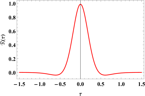
Figure 1:

Shape of the Function ${\cal R}(\tau)$ in the integrand of Eq. (5.14) (first line).

With $s=\frac{1}{2}-i\tau$ as a choice, and after some simplifications, the previous integral becomes:

$$a^{\rm QED}({\rm VP})=\left(\frac{\alpha}{\pi}\right)^{2}\frac{1}{4}\frac{1}{2\pi}\int_{-\infty}^{+\infty}d\tau\left\{\underbrace{\left[\frac{1}{1+\tau^{2}}-\frac{10}{4+\tau^{2}}+\frac{40}{25+\tau^{2}}\right]\frac{\pi^{2}}{[\cosh(\pi\tau)]^{2}}}_{\Re(\tau)}\right.$$ (5.14)

$$\left.-i\tau\left[\frac{1}{1+\tau^{2}}-\frac{5}{4+\tau^{2}}+\frac{16}{25+4\tau^{2}}\right]\frac{\pi^{2}}{[\cosh(\pi\tau)]^{2}}\right\}$$

$$=\left(\frac{\alpha}{\pi}\right)^{2}\times 0.01568742185910\,,$$

which, to this remarkable accuracy, agrees with the exact analytic result (see e.g. ref. [24]):

$$a^{\rm QED}({\rm VP})=\left(\frac{\alpha}{\pi}\right)^{2}\left(\frac{119}{36}-\frac{\pi^{2}}{3}\right)\,.$$ (5.15)

Notice that the imaginary part of the integrand in the second line of Eq. (5.14) gives zero contribution to the integral. The shape of the function ${\cal R}(\tau)$ in the first line, which is symmetric under $\tau\rightarrow-\tau$, defines the real part of the integrand and it is shown in Fig (1).

V.2 Application to Vacuum Polarization in QCD

We can now go back to QCD. As already stated in Eq. (2.2) the QCD Mellin transform ${\cal M}(s)$ is singular at $s=1$ with a residue which is fixed by pQCD. For three light $u$, $d$, $s$ quarks and neglecting ${\cal O}(\alpha_{\mbox{\rm{\scriptsize s}}})$ corrections this fixes the pQCD-Marichev Interpolation to the simple function

$${\cal M}(s)\Rightarrow{\cal M}^{(1)}(s)={\cal C}\ \frac{1}{1-s}\,,$$ (5.16)

where ${\cal C}$ will denote the overall constant

$${\cal C}\equiv\frac{\alpha}{\pi}\frac{1}{3}\ N_{c}\left(\frac{2}{3}\right)\,.$$ (5.17)

Contrary to the QED case discussed before, the ${\cal O}(1/Q^{2})$ term in the asymptotic expansion of $\Pi(Q^{2})$ for large $Q^{2}$ in QCD vanishes in the chiral limit which requires that

$${\cal M}(2)=0\,,$$ (5.18)

and the corresponding interpolation is then

$${\cal M}^{(1,2)}(s)={\cal C}\ \frac{1}{(1-s)\Gamma(2-s)}\,.$$ (5.19)

This is as much as we shall use from the short-distance behaviour of QCD.

V.2.1 First Marichev Interpolation when ${\cal M}(0)$ is known

Let us now construct the QCD equivalent of the Marichev Interpolation which in the QED example above already reproduced the exact result. This corresponds to the case where, besides ${\cal M}(1)$ and ${\cal M}(2)$, we also know the slope at the origin of the HVP-function, i.e. we know ${\cal M}(0)$. The corresponding interpolation, which in the QCD case we shall call the First Marichev Interpolation has the same functional form as the QED one in Eq. (5.9), i.e.

$${\cal M}(s)\Rightarrow{\cal M}^{(1,2)}_{(0)}(s)={\cal C}\ \frac{1}{1-s}\frac{\Gamma(c-1)}{\Gamma(c-s)}\frac{\Gamma(d-s)}{\Gamma(d-1)}\,,$$ (5.20)

but with the parameters $c$ and $d$ restricted now to satisfy the two QCD constraints at $s=2$ and $s=0$:

$$\frac{c-2}{d-2}=0\,,\quad\mbox{\rm and}\quad{\cal C}\ \frac{d-1}{c-1}={\cal M}(0)\,,$$ (5.21)

which results in

$$c=2\quad\mbox{\rm and}\quad d=1+\frac{1}{{\cal C}}\ {\cal M}(0)\,.$$ (5.22)

With ${\cal A}$ denoting the quantity:

$${\cal A}\equiv\frac{1}{{\cal C}}{\cal M}(0)\,,$$ (5.23)

the interpolation in question is then:

$${\cal M}^{(1,2)}_{(0)}(s)={\cal C}\ \frac{1}{(1-s)\Gamma(2-s)}\frac{\Gamma\left[1+{\cal A}\ -s\right]}{\Gamma\left({\cal A}\right)}\,.$$ (5.24)

One can now proceed to the determination of the corresponding prediction for $a_{\mu}^{\rm HVP}$ inserting this ${\cal M}^{(1),(2)}_{(0)}(s)$ interpolating Mellin transform in Eq. (5.13) and evaluating numerically the integral with e.g. the choice $c_{s}=\frac{1}{2}$:

$$a_{\mu}^{\rm HVP}({\rm first})=\left(\frac{\alpha}{\pi}\right)\frac{m_{\mu}^{2}}{t_{0}}\frac{1}{2\pi}\int\limits_{-\infty}^{+\infty}d\tau\left(\frac{m_{\mu}^{2}}{t_{0}}\right)^{-\left(\frac{1}{2}-i\tau\right)}{\cal F}\left(\frac{1}{2}-i\tau\right)\ {\cal M}^{(1,2)}_{(0)}\left(\frac{1}{2}-i\tau\right)\,,$$ (5.25)

where ${\cal F}(s)$ is the function defined in Eq. (3.16).

V.2.2 Second Marichev Interpolation when ${\cal M}(0)$ and ${\cal M}(-1)$ are known

The previous interpolation can be improved once we know both the slope and the curvature of $\Pi^{\rm HVP}(Q^{2})$ at the origin i.e. when ${\cal M}(0)$ and ${\cal M}(-1)$ are known, in which case we use as an ansatz the following Second Marichev Interpolation:

$${\cal M}(s)\Rightarrow{\cal M}^{(1,2)}_{(0,-1)}(s)={\cal C}\ \frac{1}{1-s}\frac{1}{\Gamma(2-s)}\frac{\Gamma(e-s)}{\Gamma(e-1)}\frac{\Gamma(f-1)}{\Gamma(f-s)}\,,$$ (5.26)

with the $e$ and $f$ parameters fixed by the matching equations:

$${\cal M}^{(1,2)}_{(0,-1)}(0)={\cal M}(0)\quad\mbox{\rm and}\quad{\cal M}^{(1,2)}_{(0,-1)}(-1)={\cal M}(-1)\,.$$ (5.27)

In terms of the quantities ${\cal A}$ (defined in Eq. (5.23)) and the ratio:

$${\cal R}=4\frac{{\cal M}(-1)}{{\cal M}(0)}\,,$$ (5.28)

we find

$$f=\frac{1-{\cal A}}{{\cal R}-{\cal A}}\,,\quad\mbox{\rm and}\quad e={\cal R}f\,.$$ (5.29)

The corresponding prediction for $a_{\mu}^{\rm HVP}$ is then given by the numerical evaluation of the integral (which is in fact a Fourier-like transform):

$$a_{\mu}^{\rm HVP}({\rm second})=\left(\frac{\alpha}{\pi}\right)\frac{m_{\mu}^{2}}{t_{0}}\frac{1}{2\pi}\int\limits_{-\infty}^{+\infty}d\tau\left(\frac{m_{\mu}^{2}}{t_{0}}\right)^{-\left(\frac{1}{2}-i\tau\right)}{\cal F}\left(\frac{1}{2}-i\tau\right)\ {\cal M}^{(1,2)}_{(0,-1)}\left(\frac{1}{2}-i\tau\right)\,.$$ (5.30)

We wish to emphasize that the first and second Marichev functions in Eqs. (5.24) and (5.26) are unique in the sense that, with the information provided, they are the most general Mellin transforms satisfying the criteria stated after Eq. (5.1).

We have now all the ingredients to test these First and Second Marichev Interpolations with phenomenological models, and then to apply them to the evaluation of $a_{\mu}^{\rm HVP}$ using as an input the recent LQCD determinations [13] of ${\cal M}(0)$ and ${\cal M}(-1)$.

VI Tests with a Phenomenological Model

In order to test the interpolation approach proposed above, we shall apply it to a phenomenological model of the hadronic spectral function, which we call the Toy Model [14]. The model has been constructed to simulate the basic features of the phenomenological spectral function, but with fixed parameters (i.e. no errors) so as to be handled mathematically as an exact function. The Toy Model spectral function in the low energy range below $1~{}\mbox{\rm GeV}^{2}$ is shown in Fig. (2). Although this Toy Model should not be confused with the experimental determination of the spectral function, beautifully shown e.g. in ref. [10], it reproduces nevertheless rather well its phenomenological features and, for our purposes, it can be considered as a good theoretical test laboratory.

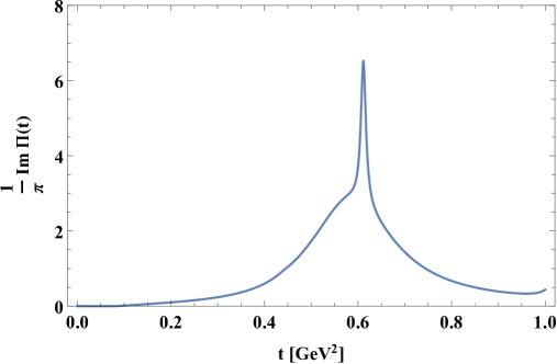
Figure 2:

The Toy Model Spectral Function below $1~{}\mbox{\rm GeV}^{2}$

We first observe that, by contrast to the complex structure of the spectral function of the Toy Model shown in Fig. (2), its Mellin transform, which is shown in Fig. (3), has an extraordinarily smooth shape. In particular, the value at $s=0$, which corresponds to the slope of the $\Pi^{\rm HVP}(Q^{2})$-function at the origin and which we shall use later is

$${\cal M}^{\rm ToyM}(0)=0.7057904\times 10^{-3}\,.$$ (6.1)

The value at $s=-1$, which corresponds to the curvature of the same $\Pi^{\rm HVP}(Q^{2})$-function at the origin (the second derivative) and which we shall also use later is

$${\cal M}^{\rm ToyM}(-1)=0.1151594\times 10^{-3}\,.$$ (6.2)

For $0\leq\mbox{\rm Re}(s)<1$ the Mellin transform continues to rise monotonously to become singular at $s=1$ as predicted by pQCD.

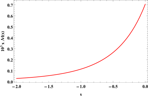
Figure 3:

Mellin Transform of the Toy Model Spectral Function (including charm).

Using the standard representation of $a_{\mu}^{\rm HVP}$ in Eq. (3.1) we find that the Toy Model predicted value of the HVP contribution to the muon anomaly is

$$a_{\mu}^{\rm HVP}({\rm ToyM})=6.812175\times 10^{-8}\,,$$ (6.3)

somewhat smaller than the determinations using $e^{+}e^{-}$ data in Eqs. (1.12) which, in fact, have some extra contributions included; but, as already said, the purpose of the model is not to reproduce experimental results but rather to be used as a testing theoretical laboratory.

The Toy Model above has four active flavours: the three light quarks $u$, $d$, $s$ and the heavy charm quark with mass $M_{c}$. On the other hand, the Marichev interpolations that we have discussed in the previous section are for three light flavours $u$, $d$, $s$. Therefore, in order to compare it with the Toy Model, we have to subtract from it the charm quark $c$ contribution. This we do by observing that the effective charm-quark contribution is well described by a constituent charm quark model with a spectral function

$$\frac{1}{\pi}\mbox{\rm Im}\Pi_{c}(t)=\frac{\alpha}{\pi}\frac{1}{3}\ N_{c}\left(\frac{4}{9}\right)\left(1+\frac{2M_{c}^{2}}{t}\right)\sqrt{1-\frac{4M_{c}^{2}}{t}}\ \theta(t-4M_{c}^{2})\,,$$ (6.4)

with (we shall use for $M_{c}$ its central value)

$$M_{c}=(1.275\pm 0.025)~{}\mbox{\rm GeV}\,.$$ (6.5)

This gives a contribution to the Mellin transform:

$${\cal M}^{\rm charm}(s) = \int_{t_{0}}^{\infty}\frac{dt}{t}\left(\frac{t}{t_{0}}\right)^{s-1}\frac{1}{\pi}\mbox{\rm Im}\Pi_{c}(t)=\left(\frac{4M_{c}^{2}}{t_{0}}\right)^{s-1}\int_{4M_{c}^{2}}^{\infty}\frac{dt}{t}\left(\frac{t}{4M_{c}^{2}}\right)^{s-1}\frac{1}{\pi}\mbox{\rm Im}\Pi_{c}(t)$$ (6.6)

$$= \frac{\alpha}{\pi}\frac{1}{3}\ \mbox{${\rm N_{c}}$}\left(\frac{4}{9}\right)\left(\frac{4M_{c}^{2}}{t_{0}}\right)^{s-1}\frac{1}{1-s}\frac{3\sqrt{\pi}}{4}\frac{\Gamma(3-s)}{\Gamma(\frac{7}{2}-s)}\,,\quad-\infty\leq\mbox{\rm Re}(s)<1\,,$$

and the Mellin transform of the Toy Model spectral function to compare with should, therefore, be:

$${\cal M}(s)={\cal M}^{\rm ToyM}(s)-{\cal M}^{\rm charm}(s)\,,$$ (6.7)

which results in the following values for the constants ${\cal A}$ and ${\cal R}$ defined in Eqs. (5.23) and (5.28):

$${\cal A}=0.449485\quad\mbox{\rm and}\quad{\cal R}=0.661645\,.$$ (6.8)

Furthermore, the contribution to the muon anomaly from the charm spectral function in Eq. (6.4) with $M_{c}=1.275~{}\mbox{\rm GeV}$, using e.g. the standard representation in Eq. (3.1), is

$$a_{\mu}^{\rm HVP}({\rm charm})=0.1094352\times 10^{-8}\,,$$ (6.9)

which also has to be subtracted as well from the one in Eq. (6.3). More precisely, the predictions for the muon anomaly using the Marichev interpolation will be compared to the value

$$a_{\mu}^{\rm HVP}=a_{\mu}^{\rm HVP}({\rm ToyM})-a_{\mu}^{\rm HVP}({\rm charm})=6.70274\times 10^{-8}\,.$$ (6.10)

At this level it is interesting to compare the Mellin transform of the Toy Model with those corresponding to the two Marichev interpolations in Eqs. (5.24) and (5.26). This is shown in Fig. (4) below. One can see a net improvement from the first interpolation (the green curve) to the second one (the blue curve) which is already quite close to the Toy Model one (the red curve).

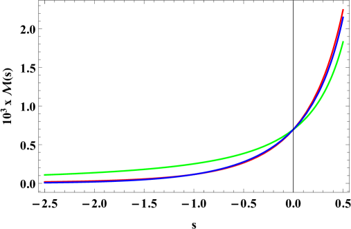
Figure 4:

Mellin Transforms of the Hadronic Spectral Function
Red: Toy Model without Charm
Green: Marichev’s Interpolation with only ${\cal M}(0)$ as input
Blue: Marichev’s Interpolation with ${\cal M}(0)$ and ${\cal M}(-1)$ as input.

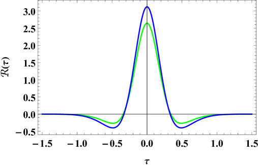
Figure 5:

Shape of the Functions $\Re^{1,2}_{0}(\tau)$ (green curve)and $\Re^{1,2}_{0,-1}(\tau)$ (blue curve)

It is also interesting to show the shapes of the real parts of the integrands in Eqs. (5.25) and (5.30) as functions of $\tau$ corresponding to the First and Second Marichev Interpolations, i.e. the functions

$$\Re^{1,2}_{0}(\tau) = \frac{1}{{\cal C}}\left(\frac{m_{\mu}^{2}}{t_{0}}\right)^{-\left(\frac{1}{2}-i\tau\right)}{\cal F}\left(\frac{1}{2}-i\tau\right)\ {\cal M}^{(1,2)}_{(0)}\left(\frac{1}{2}-i\tau\right)$$ (6.11)

$$\Re^{1,2}_{0,-1}(\tau) = \frac{1}{{\cal C}}\left(\frac{m_{\mu}^{2}}{t_{0}}\right)^{-\left(\frac{1}{2}-i\tau\right)}{\cal F}\left(\frac{1}{2}-i\tau\right)\ {\cal M}^{(1,2)}_{(0,-1)}\left(\frac{1}{2}-i\tau\right)\,,$$ (6.12)

where for convenience we have factorized the overall constant ${\cal C}$ in Eq. (5.17). The shapes of the real parts of these two functions of $\tau$ are shown in Fig.(5). The green curve corresponds to $\Re^{1,2}_{0}(\tau)$, the blue curve to $\Re^{1,2}_{0,-1}(\tau)$

The result we get for $a_{\mu}^{\rm HVP}$ using the First Marichev Interpolation given by Eq. (5.24), i.e. the one corresponding to the curves in green in Figs. (4) and (5), is

$$a_{\mu}^{\rm HVP}({\rm first})=6.25021\times 10^{-8}\,.$$ (6.13)

It reproduces the Toy Model value at the 6.6% level. Not competitive enough for a comparison with the experimental results, but a net improvement with respect to the upper bound [27] value:

$$a_{\mu}^{\rm HVP}\leq\left(\frac{\alpha}{\pi}\right)\frac{m_{\mu}^{2}}{t_{0}}\frac{1}{3}{\cal M}(0)=7.72132\times 10^{-8}\,.$$ (6.14)

Notice that, at this level of approximation, i.e. with only ${\cal M}(0)$ known, there is no possible prediction from Padé approximants.

Things get much better at the level of the Second Marichev Interpolation which results in the value

$$a_{\mu}^{\rm HVP}({\rm second})=6.74591\times 10^{-8}\,,$$ (6.15)

and reproduces the Toy Model value at the 0.6% level. We find this very encouraging!

VI.1 Test with the BHLS Model of ref. [21].

One may perhaps suspect that the reason for the success of the previous results is due to the particular choice of the Toy Model as a reference. We have, therefore, also considered another phenomenological model as an alternative reference: the so called BHLS-Model of ref. [21], and applied the same method to it. For that we choose the entries corresponding to what the authors of ref. [21] call Data Direct. The values quoted for the first two moments are:

$${\cal M}(0)_{\rm BHLS} = (10.1307\pm 0.0745)\times 10^{-5}\,,$$ (6.16)

$${\cal M}(-1)_{\rm BHLS} = (0.23507\pm 0.00185)\times 10^{-5}\,,$$ (6.17)

and the corresponding result for the muon anomaly which they find is

$$a_{\mu}^{\rm HVP}({\rm BHLS})=(683.50\pm 4.75)\times 10^{-10}\,.$$ (6.18)

The central values of the BHLS-moments, in our normalization ($t_{0}=4m_{\pi^{\pm}}^{2}$), correspond to

$${\cal M}(0)=0.707094\times 10^{-3}\quad\mbox{\rm and}\quad{\cal M}(-1)=0.011452\times 10^{-3}\,.$$ (6.19)

Using these moments as an input, the result for $a_{\mu}^{\rm HVP}$ from the first Marichev approximation, the one which only requires ${\cal M}(0)$ as an input, is

$$a_{\mu}^{\rm HVP}({\rm first})=626.12\times 10^{-10}\,.$$ (6.20)

Using the second Marichev approximation, which requires both ${\cal M}(0)$ and ${\cal M}(-1)$ as input, we find

$$a_{\mu}^{\rm HVP}({\rm second})=676.32\times 10^{-10}\,,$$ (6.21)

in agreement with the BHLS value in Eq. (6.18) at the 1% level. With the charm contribution in Eq. (6.9) subtracted to the BHLS value in Eq. (6.18) the agreement is at the 0.6% level, much the same as in the case of the Toy Model.

VI.2 An Application to the LQCD Prediction of ref. [13].

Let us now apply the Marichev interpolation technique to recent LQCD results. The lattice QCD BMWc collaboration has recently published results on the first two moments ${\cal M}(0)$ and ${\cal M}(-1)$. Their numbers [13]:

$$\Pi_{1}[\mbox{\rm GeV}^{-2}]=0.0999(10)(9)(23)(13)\quad\mbox{\rm and}\quad\Pi_{2}[\mbox{\rm GeV}^{-4}]=-0.181(6)(4)(10)(2)\,,$$ (6.22)

when expressed in the normalization ($t_{0}=4m_{\pi^{\pm}}^{2}$) of our Mellin Moments, with the charm contribution subtracted, and with their errors added quadratically, correspond to the values:

$${\cal M}(0)_{{\cite[cite]{[\@@bibref{}{Lellouch16}{}{}]}}}=(0.704\pm 0.021)\times 10^{-3}\quad\mbox{\rm and}\quad{\cal M}(-1)_{{\cite[cite]{[\@@bibref{}{Lellouch16}{}{}]}}}=(0.101\pm 0.007)\times 10^{-3}\,.$$ (6.23)

These numbers result in the following values for the parameters

$${\cal A}=0.455\pm 0.014\quad\mbox{\rm and}\quad{\cal R}=0.572\pm 0.043\,,$$ (6.24)

in Eqs. (5.23) and (5.28) and are the ones to be inserted in the First and Second Marichev Interpolations in Eqs. (5.24) and (5.26).

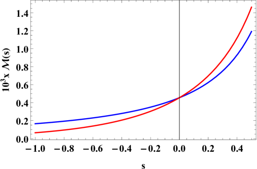
Figure 6:

Mellin Transforms corresponding to the Marichev Interpolations
using as an input the central values of the LQCD results of ref. [13].
Blue is the first interpolation, Red the second one.

Figure (6) shows the Mellin transforms obtained with the central values of the numbers above; here the blue curve corresponds to the First-Interpolation, the red curve to the improved Second-Interpolation. These curves are rather similar to the ones in Fig. (4) which test the Toy Model.

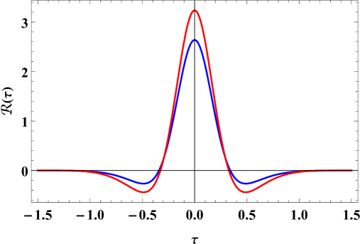
Figure 7:

Shape of the Functions $\Re^{1,2}_{0}(\tau)$ (blue curve)and $\Re^{1,2}_{-1,0}(\tau)$ (red curve)
using as an input the central values of the LQCD results of ref. [13].

Figure (7) shows the shapes of the real parts of the functions $\Re^{1,2}_{0}(\tau)$ and $\Re^{1,2}_{0,-1}(\tau)$ in Eqs. (6.11) and (6.12) using the central values of the LQCD results in ref. [13]. It is interesting that, although these shapes differ in detail from the ones corresponding to the Toy Model in Fig. (5) and from the QED one in Fig. (1) they are qualitatively rather similar. This is probably due to the fact that they all have in common the Gamma-function structure of the Marichev general ansatz in Eq. (5.1).

The corresponding predictions for $a_{\mu}^{\rm HVP}$ using the first and second interpolations, with the values of the moments in Eq. (6.23) in which the charm contributions have been subtracted, are:

$$a_{\mu}^{\rm HVP}({\it First})=(6.23\pm 0.18)\times 10^{-8}\,,$$ (6.25)

and

$$a_{\mu}^{\rm HVP}({\it Second)}=(6.81\pm 0.30)\times 10^{-8}\,.$$ (6.26)

The error in $a_{\mu}^{\rm HVP}({\it First})$ is an average of the two limits of error induced by the error in ${\cal M}(0)$. The error in $a_{\mu}^{\rm HVP}({\it Second)}$ is sensitive to both the errors in ${\cal M}(0)$ and ${\cal M}(-1)$; it has been estimated by evaluating $a_{\mu}^{\rm HVP}$ with the limit of errors in ${\cal M}(0)$ in Eq. (6.23) keeping the central value of ${\cal M}(-1)$, then evaluating $a_{\mu}^{\rm HVP}$ with the limit of errors in ${\cal M}(-1)$ in Eq. (6.23) keeping the central value of ${\cal M}(0)$ and finally averaging the partial errors quadratically. We find these results very encouraging to pursue with more accurate LQCD determinations of ${\cal M}(0)$ and ${\cal M}(-1)$ and, if possible, with the determination of higher moments.

VII Conclusions.

We conclude from this work that with a precise determination of the first Mellin Moment ${\cal M}(0)$ i.e., with a precise determination of just the slope of the HVP function at the origin accessible to LQCD, one can already obtain a result for $a_{\mu}^{\rm HVP}$ which provides a first rough test of the determinations using experimental data. Notice that in the First Marichev Interpolation, besides the eventual determination of ${\cal M}(0)$, one only uses as further information two well known properties of QCD: asymptotic freedom and the fact that in the chiral limit there is no $1/Q^{2}$ term in the OPE of $\Pi(Q^{2})$. With such limited input there is no prediction from Padé approximants one can compare with.

The Second Marichev Interpolation of the Mellin Transform of the hadronic spectral function which we have developed above results in a much more accurate determination. It includes as an input the determinations of the first two moments ${\cal M}(0)$ and ${\cal M}(-1)$, i.e. the determination of the first two derivatives of the HVP function $\Pi(Q^{2})$ at $Q^{2}=0$ accessible to LQCD. The test with the Toy Model above results in a determination of $a_{\mu}^{\rm HVP}$ with an accuracy of $0.6\%$ which is very encouraging. The application to the determination of the ${\cal M}(0)$ and ${\cal M}(-1)$ moments from LQCD [13] points towards a very promising future in this direction.

It would be very helpful to be able to test the Marichev Interpolation Approach with real experimental data. In that respect we encourage our colleagues of refs. [8, 9] to publish the values of a few moments: ${\cal M}(0)$, ${\cal M}(-1)$, ${\cal M}(-2)\,,\cdots$ of the same physical spectral function which they use for their determination of $a_{\mu}^{\rm HVP}$.

Acknowledgments.

I am very much indebted to David Greynat for many helpful comments and suggestions on the topics discussed in this paper; in particular for bringing to my attention Ramanujan’s Master Theorem. I have also benefited from discussions with Laurent Lellouch, who has kindly provided the code of his Toy Model, and with Marc Knecht and Santi Peris. I wish to thank David Greynat and Laurent Lellouch for a careful reading of the successive versions of the manuscript.

References

- [1] B.E. Lautrup, A. Peterman and E. de Rafael, Phys. Rep. C3 (1972) 193.
- [2] E. de Rafael, Phys. Lett. B322 (1994) 239.
- [3] M. Knecht, S. Peris and E. de Rafael, Phys. Lett. B443 (1998) 255.
- [4] T. Das, G.S. Guralnik, V.S. Mathur, F.E. Low and J.E. Young, Phys. Rev. Lett. 18 (1967) 759.
- [5] E. de Rafael, Nucl. Phys. (Proc. Suppl.) B119 (2003) 71.
- [6] G.W. Bennett et al. (The -2 Collab.), Phys. ReV. D73 (2006) 072003.
- [7] Th. Blum, A. Denig, I. Logashenko, E. de Rafael, B. Lee Roberts, Th. Teubner and G. Venanzoni, The Muon Theory Value: Present and Future, arXiv:1311.2198v1 [hep-ph].
- [8] M. Davier, A. Hoecker, B. Malaescu, and Z. Zhang, Eur. Phys.J. C71 (2011) 1515.
- [9] K. Hagiwara, R. Liao, A.D. Martin, D. Nomura and T.K. Teubner, J. Phys G38 (2011) 085003.
- [10] M. Davier, Update of the Hadronic Vacuum Polarization Contribution to the muon , arXiv:1612.02743v2 [hep-ph].
- [11] F. Burger, X. Feng, G. Hotzel, K. Jansen, M. Petschlies and D.B. Renner, (ETM Collaboration), JHEP 02 (2014) 099.
- [12] B. Chakraborty, C.T.H. Davis, P.G. de Oliveira, J. Koponen and G.P. Lepage, (HPQCD collaboration), arXiv:1601.03071 [hep-lat].
- [13] Sz. Borsanyi, Z. Fodor, T. Kawanai, S. Krieg, L. Lellouch, R. Malak, K. Miura, K.K. Szabo, C. Torrero and B. Toth, arXiv:1612.02364v1 [hep-lat].
- [14] L. Lellouch, Private Comunication.
- [15] B. Berndt. Ramanujan’s Notebooks, Part I. Springer-Verlag, New York, 1985.
- [16] O.I. Marichev, Handbook of Integral Transforms of Higher Transcendental Functions: Theory and Algorithmic Tables, Ellis Horwood Ltd., Chichester, U.K. 198.
- [17] Transforms and Applications Handbook, Third Edition, Editor-in-Chief, Alexander D. Poularikas, CRC Press 2010. Ch 12: J Bertrand, P. Bertrand and J-Ph Ovarlez, Mellin Transform.
- [18] L.J. Slater, Generalized Hypergeometric Functions, Cambridge University Press, 1966.
- [19] D. Greynat and E. de Rafael, The Mellin-Barnes Approach to Hadronic Vacuum Polarization and , ( to be published).
- [20] E. de Rafael, Phys. Letters B736 (2014) 52.
- [21] M. Benayoun, P. David, L. DelBuono and F. Jegerlehner, arXiv:1605.04474v1 [hep-ph].
- [22] Ph. Flajolet, X. Gourdon and Ph. Dumas, Theor. Comput., Sci. 144 (1995) 3.
- [23] S. Friot, D. Greynat, and E. de Rafael, Phys. Lett. B68 (2005) 73.
- [24] J.Ph. Aguilar, D. Greynat and E. de Rafael, Phys. Rev. D77 (2008) 093010.
- [25] S. Friot and D. Greynat, J. Math. Phys. 53 (2012) 023508.
- [26] C. Bouchiat and L. Michel, J. Phys.Radium, 22 (1961) 121.
- [27] J.S. Bell and E. de Rafael, Nucl. Phys. B11 611 (1969).
- [28] T. Blum, Phys. Rev. Lett. 91 (2003) 052001.
- [29] C. Aubin, T. Blum, M. Golterman and S. Peris, Phys. Rev. D86 (2012) 054509.
- [30] M. Golterman, K. Maltman and S. Peris, Phys. Rev. D90 (2014) 074508.
- [31] C. Aubin,T. Blum, P. Chau, M. Golterman, S. Peris and C. Tu, Phys. Rev. D93 (2016) 05450.