Mixed insulating and conducting thermal boundary conditions in Rayleigh-Bénard convection

Abstract

A series of direct numerical simulations of Rayleigh-Bénard convection, the flow in a fluid layer heated from below and cooled from above, were conducted to investigate the effect of mixed insulating and conducting boundary conditions on convective flows. Rayleigh numbers between $\mbox{{Ra}}=10^{7}$ and $\mbox{{Ra}}=10^{9}$ were considered, for Prandtl numbers $\mbox{{Pr}}=1$ and $\mbox{{Pr}}=10$. The bottom plate was divided into patterns of conducting and insulating stripes. The size ratio between these stripes was fixed to unity and the total number of stripes was varied. Global quantities such as the heat transport and average bulk temperature and local quantities such as the temperature just below the insulating boundary wall were investigated. For the case with the top boundary divided into two halves, one conducting and one insulating, the heat transfer was found to be approximately two thirds of the fully conducting case. Increasing the pattern frequency increased the heat transfer which asymptotically approached the fully conducting case, even if only half of the surface is conducting. Fourier analysis of the temperature field revealed that the imprinted pattern of the plates is diffused in the thermal boundary layers, and cannot be detected in the bulk. With conducting-insulating patterns on both plates, the trends previously described were similar, however, the half-and-half division led to a heat transfer of about a half of the fully conducting case instead of two-thirds. The effect of the ratio of conducting and insulating areas was also analyzed, and it was found that even for systems with a top plate with only $25\%$ conducting surface, heat-transport of $60\%$ of the fully conducting case can be seen. Changing the 1D stripe pattern to 2D checkerboard tessellations does not result in a significantly different response of the system.

1 Introduction

Natural convection is a common and important phenomenon which is omnipresent in Nature. It leads to the transfer of internal energy, within an unstably stratified fluid layer, via a buoyancy induced flow. Ocean currents, which are driven by gradients in density and salinity (Marshall & Schott, 1999; Wirth & Barnier, 2006), and the mantle convection inside the Earth, which drives the plate tectonics and generates the geomagnetic field (McKenzie et al., 1974; Glatzmaier & Roberts, 1995), are two examples of natural convection. Even outside of our planet, at the most distant stars, convection is of tremendous importance (Spiegel, 1971; Cattaneo et al., 2003).

An idealized system that is commonly used to study natural convection, as it is mathematically well-defined and can be reproduced in a laboratory experiment, is Rayleigh-Bénard (RB) convection (Normand et al., 1977; Ahlers et al., 2009; Lohse & Xia, 2010; Chillà & Schumacher, 2012). The RB system consists of a fluid in a container, that is heated from below and cooled from above. The fluid is subject to an external gravitational field $g$. Apart from the geometric ones, this system has two non-dimensional control parameters, namely the Rayleigh number $\mbox{{Ra}}=\beta g\Delta H^{3}/\nu\kappa$, which measures the strength of the thermal driving, and the Prandtl number $\mbox{{Pr}}=\nu/\kappa$, a property of the fluid, where $\beta$ and $\kappa$ are the isobaric thermal expansion and temperature diffusivity coefficients of the fluid, $H$ the system height, $\Delta$ the applied temperature difference between the plates, and $\nu$ the kinematic viscosity. Depending on the geometry of the system, other control parameters such as the aspect ratio of the system, $\Gamma=L/H$ appear, where $L$ is a characteristic horizontal length of the system.

Above a certain critical Rayleigh number, RB flow is linearly unstable, and any perturbation will cause the onset of convection. This critical value is determined by the properties of the fluid and the boundary conditions (BC) of the RB system. If the thermal driving of the system is far above the critical Ra, the flow becomes turbulent. This dramatically increases the heat transfer with respect to the purely conductive case. Modeling this heat transfer is essential for understanding what is going on inside stars, the Earth’s mantle and many other systems. RB experiments (and simulations) typically consist of a bottom and a top plate which have homogeneous boundary conditions, and lateral boundary conditions which are either periodic (simulations) to mimic laterally unconfined systems or adiabatic (experiments) to account for a lateral confinement that minimizes the heat losses.

However, these idealized systems assume that both the top and bottom plates have perfectly homogeneous conducting surfaces while for all real physical systems, there is a certain degree of imperfection. In Nature we see such inhomogeneities; for example, the fractures in ice floes (Marcq & Weiss, 2012) or the much debated insulating effects of continents on mantle convection (Lenardic et al., 2005). Other examples include convection over mixed (agricultural) vegetation and cities (Zhao et al., 2014). In engineering applications, or in RB experiments these can be small defects or dirt at the conducting plates, which could result in lower than optimal heat transport. The limiting cases of the boundary conditions are constant heat flux boundary conditions, constant temperature boundary conditions, or thermally insulating boundary conditions with no heat flux. The difference in heat transfer between the first two types of boundary conditions, Dirichlet and von Neumann, was found to be negligible at large Ra DNS (Johnston & Doering, 2007, 2009; Stevens et al., 2011), but the increase in flow strength under fixed-temperature BC cannot be neglected (Huang et al., 2015). Accounting for a finite conductivity of the thermal sources can lead to significant reduction in the heat transport (Verzicco, 2004).

Temperature boundary conditions can also be spatially and temporally varying. The study of the effects of these imperfect boundary conditions goes back to Kelly & Pal (1978) and later Yoo & Moon (1991) who applied sinusoidal temperature boundary conditions on both plates, which mimic plates with embedded heaters. These plates are locally hotter, when closer to the heater elements. Jin & Xia (2008) showed that the Nusselt number is increased when the energy input into the system from the plates is periodically pulsed instead of stationary. Recent experiments from Wang et al. (2017) using insulating lids at the top boundary of a RB cell showed that with increasing insulating fraction the same amount of heat goes through a smaller cooling area. Some simulations of inhomogeneous boundary conditions have also been performed. Cooper et al. (2013) simulated two and three-dimensional Rayleigh-Bénard systems of mixed adiabatic-conducting boundary conditions at one plate at moderate Rayleigh numbers, with a geophysical focus, finding that the distribution of the patches caused changes in the flow configuration, the bulk temperature and the Nusselt number. The simulations by Ripesi et al. (2014) added non-conducting defects in the form of periodic patches to the top plate of a two-dimensional numerical RB system, and studied both the transition to turbulence of RB flow, finding a delay in this transition when defects were present, and the fully turbulent regime, finding a decrease in Nusselt number when the patch wavelength was larger than the characteristic thermal boundary layer scale.

Here, we extend the research of Ripesi et al. (2014) by applying non-conducting stripe patterns to a three-dimensional RB system. We will focus on the fully turbulent regime instead of the transition to turbulence, and consider a wider range of patterns at higher Ra, extending the work by Cooper et al. (2013). We start by applying distributions of striped insulating patterns to the top boundary only, and study the dependence of both local and global variables, e.g. effective heat transfer and average bulk temperature, on the number of stripes. For most of the study, we keep the conducting to insulating areas equal to each other, but the effect of this ratio is also studied, which mimics the degree of imperfections and pollution on the plates. We also study the effect of applying the same pattern to both plates and the role of the pattern geometry by applying a two-dimensional checkerboard insulating-conducting pattern on the top plate. Checkerboards and stripes can be seen as the two limiting cases for the pattern geometry.

This manuscript is organized as follows: First, in section 2 we detail the geometry and numerical method. In the next section, the results for the stripe pattern variations will be discussed where both conducting and insulating areas are kept constant. This is first done on the top plate and later the pattern is applied on both plates. A Fourier analysis was performed to study the penetration depth of the pattern imprint in the flow. In subsection 3.2 a pattern is added to both plates, in subsection 3.3, we present and discuss the results for varying the ratio of conducting to insulating surface while keeping the number of divisions constant and in subsection 3.4 we present the results for a plate with a checkerboard pattern instead of a striped pattern. The manuscript is concluded by presenting the conclusions and outlook in section 4.

2 Numerical method

In this numerical study, we solve the incompressible Navier-Stokes equations within the Boussinesq approximation for RB. In non-dimensional form, these read:

$$\frac{D\boldsymbol{u}}{Dt} =-\nabla P+\left(\frac{\mbox{{Pr}}}{\mbox{{Ra}}}\right)^{1/2}\nabla^{2}\boldsymbol{u}+\theta\hat{z},$$ (1)

$$\frac{D\theta}{Dt} =\frac{1}{\left(\mbox{{Pr}}\mbox{{Ra}}\right)^{1/2}}\nabla^{2}\theta,$$

$$\nabla\cdot\boldsymbol{u} =0,$$

where $u$ is the non-dimensional velocity, $P$ is the non-dimensional pressure, $\theta$ is the non-dimensional temperature, and $\hat{z}$ is the unit vector pointing in the direction opposite to gravity $g$. For non-dimensionalization, the temperature scale is the temperature difference between the plates $\Delta$, the length scale their distance $H$ and the velocity scale is the free-fall velocity $U_{f}=\sqrt{g\beta\Delta H}$.

We consider a geometry which is a horizontally doubly-periodic cuboid. The domain has horizontal periodicity lengths of $L_{x}$ and $L_{y}$, and a vertical dimension $H$. These variables with a tilde superscript denote their non-dimensional counterparts. The equations were discretized using an energy-conserving second-order finite-difference scheme, and a fractional time-step for time marching using a third-order low-storage Runge-Kutta scheme for the non-linear terms, and a second order Adams-Bashworth scheme for all viscous and conducting terms (Verzicco & Orlandi, 1996; van der Poel et al., 2015). The code was heavily parallelized to run on hundreds or even thousands of cores simultaneously and was validated many times (Stevens et al., 2010, 2011; van der Poel et al., 2015). Recently, the code was open-sourced and is available for download at www.AFiD.eu.

The domain was discretized by $n_{x}\times n_{y}\times n_{z}=360\times 360\times 288$ grid points. In both horizontal directions, the grid was uniformly divided, and in the vertical direction the points were clustered near the top and bottom plates. A number of simulations were conducted to test the aspect ratio dependence and the grid independence. These tests did not show any significant differences in the range of Rayleigh numbers used in this study. For RB convection, a series of exact relationships which link the Nusselt number to the global kinetic energy dissipation ($\nu\nabla^{2}u$) and the thermal dissipation ($\kappa\nabla^{2}\theta$) exist (Shraiman & Siggia, 1990; Ahlers et al., 2009), and they have been further used to check the spatial accuracy of the simulation as in Stevens et al. (2010). The size of the time steps was chosen dynamically by imposing that the Courant-Friedrichs-Lewy (CFL) number in the grid would not exceed $1.2$.

The main response of the system is the Nusselt number (Nu), which is the heat transfer non-dimensionalized using the purely conductive heat transfer:

$$\mbox{{Nu}}=\frac{\left<u_{z}\theta\right>_{A}-\kappa\partial_{z}\left<\theta\right>_{A}}{\kappa\Delta L_{z}},$$ (2)

where $\left<\cdot\right>_{A}$ indicates the average over any horizontal plane. The simulations were run between 50 and 100 large-eddy turnover times based on $U_{f}$ and $H$. Statistical convergence is assessed by calculating differences in Nu between final and half the amount of measurement points. These are shown as error bars in the plots.

In the classical RB case, both the top and bottom plates have a homogeneous boundary condition, i.e. they are perfectly conducting. Here, we use this boundary condition only for the bottom plate, while top plate is taken to have periodic patches of insulating regions which do not contribute to the heat transfer from fluid to plate. The definition of these patches are similar to those in Ripesi et al. (2014):

$$\theta(\hat{x},\hat{y},\hat{z}=1) =0 \forall\hat{x},\hat{y}\in\left[jL_{p},L_{p1}+jL_{p}\right],j\in\mathbb{Z}$$ (3)

$$\partial_{z}\theta(\hat{x},\hat{y},\hat{z}=1) =0 \forall x,y\notin\left[jL_{p},L_{p2}+jL_{p}\right],j\in\mathbb{Z}$$

$$\theta(\hat{x},\hat{y},\hat{z}=0) =1 \forall x,y.$$

Here $L_{p}$ is the width of a pair of patches. $L_{p1}$ is the width of the conducting part, $L_{p2}$ is the insulating part, and the hat on the spatial coordinates indicates non-dimensionalizations. For most of this study we keep the insulating and conducting areas equal, i.e. $\ell_{C}=1/2$. The BC on the top plate depends only on the $x$-coordinate, which results in sets of insulating and conducting stripes. The number of stripe pairs in a horizontal direction L were defined as $f=L/L_{p}$, which is a central control parameter of this study. A two-dimensional schematic is shown in Figure 1.

Figure 1: Two-dimensional $y$-cut of the geometry. The domain has the dimensions $L_{x}\times L_{y}\times H$. The bottom plate, at $\hat{z}=0$, has $\theta=1$. The top plate is divided into stripes of conducting ($\theta=0$) and insulating ($\partial_{z}\theta=0$) regions.

There are limitations on the value of $f$. As each stripe has to be an integer number of grid points, only integer multiples of the grid resolution are valid. In addition, the width of all stripes summed should fit inside the system, e.g. the width in grid points should exactly be the number of grid points in the x-direction. This results in a total of 18 different pattern frequencies. For the smallest possible frequency, $f=1$, we have one conducting and one insulating stripe, which both have a width of 180 grid points. The pattern with the largest frequency, $f=90$, has 90 stripe pairs where each stripe has a width of two grid points. In this paper we will use the wavenumber $k_{x}=\left(2\pi f\right)/L_{x}$, to describe the stripe distribution.

To give an idea of how the flow in such a system looks like, two different instantaneous snapshots of the RB system with two different stripe frequencies are shown in Figure 2. Both cases have exactly the same conducting and insulating areas, but a different stripe pattern. In section 3.4, we also vary the BC in y-direction, while keeping both the insulating and conducting areas equal, which results in a checkerboard pattern.

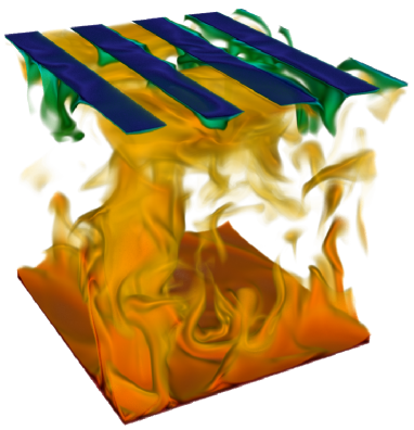
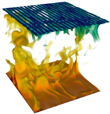
Figure 2: Two 3D visualizations of the instantaneous temperature field with different pattern frequencies applied to the top boundary. $\ell_{C}=0.5$, $\mbox{{Ra}}=10^{8}$ and $\mbox{{Pr}}=1$ for both cases. Hot fluid is shown in red while the cold fluid has a blue color. The left visualization shows $f=4$, four insulating stripes and four conducting stripes. The right visualization shows five times as many stripe pairs, with $f=20$. Plumes of colder fluid are ejected primarily from the conducting areas for $f=4$ while for $f=20$ the plumes also eject on areas below insulating regions.

3 Results

3.1 The effect of the number of stripes

In this subsection we present results of a series of simulations in which we varied the number of stripes while keeping $\ell_{C}=1/2$. Four sets of cases were run for $\mbox{{Ra}}=10^{7}$, $10^{8}$, and $10^{9}$ and $\mbox{{Pr}}=1$ and $10$.

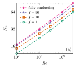
(a)

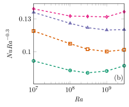
(b)

Figure 3: (a) Nusselt number $Nu$ and (b) compensated Nusselt number $NuRa^{-0.3}$ against $Ra$ for various $f$ and $Pr=1$. The markers show the actual results while the dotted lines indicate the trend between these simulations. $\ell_{C}$ was fixed to $\ell_{C}=0.5$ for all simulations.

First we show in Figure 3a the curves of Nu(Ra) for the fully conducting case and three striped cases with $f=$ 1, 10, and 90. The markers show the actual results from the simulations and the dotted lines indicate the trend between the measurements. From this figure we see that the scaling does not differ significantly between all cases and all curves are almost parallel. We do see a strong dependence on the wavenumber of the pattern. For $f=1$, we computed that Nu is approximately $2/3$ of the fully conducting case. Increasing $f$ results in a larger Nu and the values almost converge with the fully conducting case. Both the $f=90$ and $f=10$ cases are relatively closer to the fully conducting case at $\mbox{{Ra}}=10^{7}$ than at $\mbox{{Ra}}=3\times 10^{9}$. Our interpretation is that, due to the lower Ra, the thermal BL is thicker which results in larger horizontal conduction of heat. As all curves have approximately the same scaling we have compensated the data using $\mbox{{Ra}}^{-0.3}$, which is shown in figure 3b. Here it is clearly visible that for low Ra, the $f=90$ case is almost as efficient as the fully conducting case, but the differences increase with increasing Ra. The two extreme cases, $f=1$ and the fully conducting case, follow a similar trend, however, the $f=1$ case is shifted to a lower, less efficient level. Both figures clearly show that an increase in wavenumber of the pattern results in an increase in Nu.

To make this point even more clear, we plotted Nu($k_{x}$) in figure 4a. All datasets show a clear $k_{x}$ dependence: Nu quite strongly increases with $k_{x}$. The gray area indicates the data points for which the width of the stripes $L_{p}$ is smaller than the thermal boundary layer thickness $\lambda_{T}$, which can be estimated as $\lambda_{T}=H/(2\mbox{{Nu}})$. Ripesi et al. showed that the heat transfer monotonically increases with increasing $k_{x}$ until $L_{p}$ is comparable to $\lambda_{T}$. A similar trend is visible for $\mbox{{Ra}}=$1\text{\times}{10}^{7}$$ and $\mbox{{Ra}}=$1\text{\times}{10}^{8}$$ even if the $\mbox{{Ra}}=$1\text{\times}{10}^{7}$$ case shows minor increases in heat transfer when $L_{p}$ is further decreased beyond $\lambda_{T}$. The change in Pr from $\mbox{{Pr}}=1$ to $\mbox{{Pr}}=10$ does not have a significant effect for the heat transfer, at least not for $\mbox{{Ra}}=10^{8}$, for which the two datasets are practically overlapping. This behavior is similar to the standard Rayleigh-Bénard case, in which the Pr of Nu is also weak (Ahlers et al., 2009).

To perform a better comparison between the different Ra, we normalize the resulting Nu using $\mbox{{Nu}}_{fc}$, the Nusselt number of the fully conducting case. The normalized Nu for different stripe configurations are shown in figure 4b. We see the same trend for all Ra and Pr. At the lowest $k_{x}$, in which we only have a single conducting and single insulating stripe, the effective Nu is approximately two-thirds of the fully conducting case. When the number of stripes, i.e. $k_{x}$, is increased, we see that for all tested Ra and Pr, the Nusselt number slowly converges to almost the fully conducting case. So remarkably even if only half of the plate is conducting, it can be almost as effective as if the plate is fully conducting. In this compensated plot it is also clearly visible that for the largest $k_{x}$ of $\mbox{{Ra}}=$1\text{\times}{10}^{7}$$, for which $L_{p}$ goes below the size of $\lambda_{T}$, the heat transfer is still increasing.

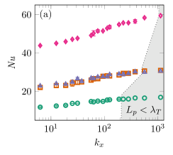
(a)

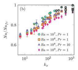
(b)

Figure 4: (a) Nusselt number Nu for various Ra and Pr versus pattern wavenumber $k_{x}$. The shaded area shows the data points for which the stripe width is smaller than the thermal boundary layer. (b) The same data but normalized by $\mbox{{Nu}}_{fc}$. The dark points are the same as in the shaded area of 4a. For both plots, the error bars shows the statistical convergence error.

The differences between the different Ra are not so clear at the lowest $k_{x}$; however, for a slight increase of $k_{x}$ we see that the curves order themselves. $\mbox{{Ra}}=10^{9}$ increases slightly slower with $k_{s}$ when comparing it to the $\mbox{{Ra}}=10^{8}$ case. The $\mbox{{Ra}}=10^{7}$ case increases slightly faster than the $\mbox{{Ra}}=10^{8}$ case and it ends at 99.7% of the fully conducting case for the largest number of stripes used. The explanation for this trend is the difference in boundary layer thickness, which decreases when we increase Ra. The boundary layer controls the heat transport from the bulk to the conducting region. Below the insulating region, this heat transport must also go in the horizontal direction. By increasing Ra and thus decreasing the thickness of the boundary layer, the same amount of heat needs to be conducted through a smaller ’channel’. This explains the decreased effectiveness with increasing Ra.

In these sets of simulations, we also compare $\mbox{{Pr}}=10$ with $\mbox{{Pr}}=1$ for $\mbox{{Ra}}=10^{8}$. The results for both Pr are quite similar. At lower $k_{x}$, we see that the $\mbox{{Pr}}=10$ case has only a marginally larger Nu and these differences become smaller with increasing $k_{x}$ and are within the uncertainty of the simulation.

Figure 5a shows the average bulk temperature of the fluid plotted against the wavenumber. This average was computed over the horizontal plane at mid-height of the system. The effect is similar to what we see for $\mbox{{Nu}}/\mbox{{Nu}}_{fc}$ in figure 4b. At the lowest $k_{x}$ the average bulk temperature has increased to about $2/3$. In that case top plate is split in half and only one half is contributing to heat transfer. While ignoring the adiabatic area, we can divide the conducting areas into three equally sized parts with two parts on the bottom plate and one on the top plate. Using the same reasoning to that used for the symmetric case, we obtain the following equality for the average bulk temperature: $\theta_{bulk}=\frac{2}{3}\theta_{bottom}+\frac{1}{3}\theta_{top}=2/3$. As with $\mbox{{Nu}}/\mbox{{Nu}}_{fc}$, we see that the average bulk temperature approaches the fully conducting case of $\theta_{bulk}=1/2$ for increasing $k_{x}$. When comparing the various curves, they all appear similar, with a maximum difference of about 0.02 to 0.03 in the average bulk temperature. Unfortunately, Wang et al. (2017) do not report their average temperature and a comparison to their calculations with large-wavelength imperfect boundary conditions is impossible.

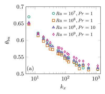
(a)

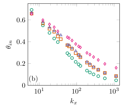
(b)

Figure 5: (a) Temperature of the bulk fluid $\theta_{bu}$ for various Nu and Pr versus pattern wavenumber $k_{x}$. (b) Temperature below the insulating stripes $\theta_{in}$, averaged over the entire insulating area, for different Ra and Pr against pattern wavenumber $k_{x}$.

In figure 5b we show the horizontally and time averaged temperature below the insulating area of the top plate as function of the wavenumber. At the lowest wavenumber (top plate split into equal conducting and insulating regions), we see that the averaged temperature is almost equal for all Ra and Pr. When increasing $k_{x}$, a dependence on Ra emerges. After just a few additional divisions in stripes, all curves order themselves according to Ra, with the lower Ra values approaching the lower bounds faster than the larger ones. At the largest $k_{x}$, the temperature difference between $\mbox{{Ra}}=10^{9}$ and $\mbox{{Ra}}=10^{7}$ is 15%. As the temperature below the insulating area is slightly higher than for the area below the conducting area because of lack of cooling, we can conclude that for larger Ra, the whole top layer is, on average, hotter than for the lower Ra.

These results suggest that it could be possible to account for the $\mbox{{Nu}}(k_{x})$ relationship by using corrected non-dimensional variables in the spirit of Verzicco (2004). However, changing the (effective) thermal conductivity, ignores the heterogeneities of the plate which is the main source of the observed behavior. In figure 6, we show the corrected Nusselt number $\mbox{{Nu}}^{*}=\mbox{{Nu}}/\theta^{*}$ against the corrected Rayleigh number $\mbox{{Ra}}^{*}=\mbox{{Ra}}\theta^{*}$, where $\theta^{*}$ is the non-dimensional average temperature difference given by $\theta^{*}=L_{p2}\theta_{in}/L_{p}$. No logical ordering can be seen, and as expected, an attempt to describe the results with some global effective thermal conductivity fails.

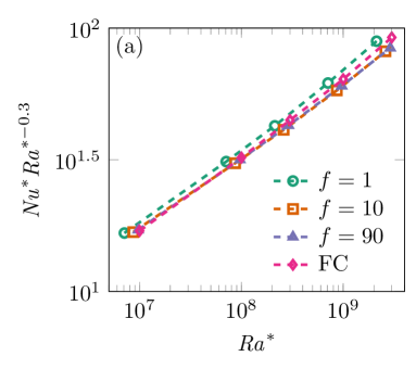
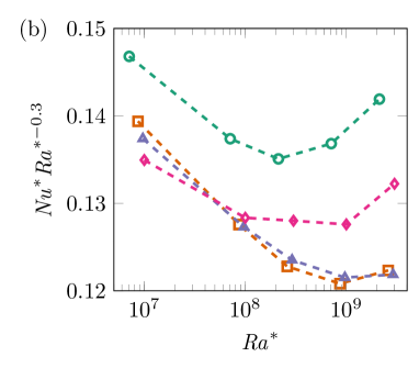
Figure 6: (a) Corrected Nusselt number against compensated Rayleigh number for selected pattern wavelengths. (b): Compensated and corrected Nusselt number against corrected Rayleigh number. No collapse, or natural ordering of the curves can be seen.

For horizontal slices of the instantaneous temperature field, a discrete two-dimensional Fourier transform can be applied, which is defined as:

$$\Theta(\gamma)=\left|\left<\sum\limits_{y=0}^{n_{y}-1}\sum\limits_{x=0}^{n_{x}-1}e^{-i\left[(2\pi/n_{x})j_{x}x+(2\pi/n_{y})j_{y}y\right]}\theta(x,y,t)\right>_{t}\right|_{j_{x}=\gamma,j_{y}=0}$$ (4)

where $\left<.\right>_{t}$ is the time average and the $j_{y}$ mode was set to zero, leaving a single wavenumber parameter $\gamma\equiv j_{x}$. Using the described method on the horizontal slice just below the top boundary we can identify the imprint the stripe structured BC leave on the flow.

Using the Fourier transform we one identify the imprint of the BC just below the top boundary in the flow itself. Using this distinct signature we can find out how far this pattern is still present once one moves away from the boundary wall. The distance from the top boundary wall is indicated using $\hat{z}$. In figure 7, we see the compensated spectra for $f=1$ at five different planes for increasing $\hat{z}$. The colors are used to identify the different modes and except for figure 7d) are compiled using a single dataset (odd or even value). When moving away from the wall, we see that the two distinct modes approach each other and just outside the boundary layer, at $\hat{z}=0.970$, it is hard to distinct the two different curves at all. Within the boundary layer the signature of the pattern almost completely fades away and in the bulk flow is not visible at all. The difference between the Fourier transform just outside the BL ($\hat{z}=0.970$) and at mid-height of the system ($\hat{z}=0.5$) is marginal. These findings hold for the complete range of $f$.

It is quite remarkable that even for the most extreme case at $f=1$, the pattern is not visible in the bulk region. This means that in the boundary layer, in which conduction dominates, the temperature differences of the top plate are averaged such that an effective, slightly higher cold plate is seen by the bulk flow.

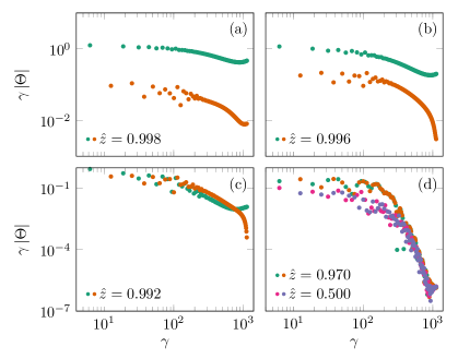
Figure 7: Premultiplied two-dimensional Fourier transform of a horizontal slice at various distances from the top boundary wall, averaged in time. Except for figure 7d, each figure is compiled using a single dataset. The colors help to identify the different modes which are present in each single dataset and are identified by the odd or even value. a) At the closest gridpoint ($\hat{z}=0.998$), the two different modes are clearly visible. b) One gridpoint further ($\hat{z}=0.996$), the distinction slowly fades. c) While still inside the boundary layer at $\hat{z}=0.992$, both modes are practically overlapping. d) Just outside the boundary layer, it is impossible to distinguish two different modes at all. As a reference, we also show the spectrum at the centre of the system ($\hat{z}=0.5$).

3.2 Patterns on both plates

Until now we only applied the insulating and conducting patches to the top boundary. This resulted in a normalized heat transfer of approximately two-thirds for the lowest $k_{x}$ and almost the fully conducting case at the highest $k_{x}$. Using a simple argument we could indeed rationalize the value of two-thirds for the normalized heat transfer for the lowest wavenumber. If we now apply the same pattern also on the bottom plate, can we still get to the same efficiency as if we only applied the pattern to the top boundary wall?

The comparison of the normalized Nusselt number $\mbox{{Nu}}/\mbox{{Nu}}_{fc}$ between the single- and double-sided case is shown in figure 8a. For the lowest $k_{x}$ we see that the double-sided case conducts heat at approximately half the rate of the fully conducting case. This is in line with the expectations, as we only have half the effective area on both boundary walls. What also is visible is that the curve for the double-sided case is steeper than the curve of the single-sided case and therefore reducing the difference between both cases with increasing $k_{x}$. For the largest $k_{x}$ the heat transfer of this system again is almost as efficient as if it were fully conducting. There is only half of the area available for heat entering the system and only half the area for heat leaving the system. Still, the same amount of heat transfer as if the system were fully conducting is achieved. For the single-sided case as for the double-sided one, for the lowest $k_{x}$ the efficiency is not exactly $2/3$ and $1/2$ but slightly above these values. The geometry of the double-sided case can be decomposed into a regular Rayleigh-Bénard cell and a neutral domain, both with identical dimensions, positioned next to each other. The top and bottom boundaries from this neutral domain are both insulating and heat can only enter and exit from the sides. As we have periodic BC in the horizontal direction, both sides of the regular RB area are connected to this neutral domain which acts as a buffer for heat. This extra buffer is the only difference and thus the cause for the small difference.

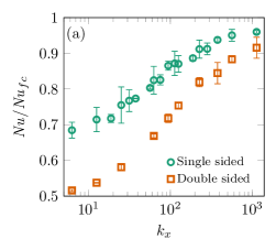
(a)

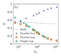
(b)

Figure 8: (a) Comparison of the normalized Nusselt number $\mbox{{Nu}}/\mbox{{Nu}}_{fc}$ for the single and double-sided cases with $\mbox{{Ra}}=10^{8}$, $\mbox{{Pr}}=1$, and $\ell_{C}=0.5$. For the lowest $k_{s}$ we see that the system is about $2/3$ and $1/2$ of the fully conducting case for the single and double-sided case, respectively. (b) Average temperature above or below the insulating stripes for the single- and double-sided case with $\mbox{{Ra}}=10^{8}$, $\mbox{{Pr}}=1$, and $\ell_{C}=0.5$. The dashed line shows the average bulk temperature, calculated at mid-height for the double-sided system.

The average temperature just below or above the insulating boundaries are shown against $k_{x}$ in figure 8b. The difference in temperature below the top insulating boundary between the single-sided case, shown in green cirlces , and the double-sided case shown in orange squares is only significant at the lowest $k_{x}$. Only at the lower $k_{x}$, the single-sided system is hotter, just below the boundary. At larger $k_{x}$, the asymmetry does not make a difference on the temperatures and both temperatures converge to the conducting plate temperature. In the same plot, we also show the temperature just above the insulating area of the bottom plate and the bulk temperature. For the double-sided case for the lowest $k_{x}$, the top, bottom, and bulk temperatures are very similar. This indicates that for the lowest $k_{x}$ all the fluid in neutral domain, the large area confined by the insulating bottom and top plate, has approximately the same temperature and hardly contributes to the heat transfer. This fully agrees with $\mbox{{Nu}}/\mbox{{Nu}}_{fc}\approx 0.5$ seen in figure 8a. The bulk temperature of the double-sided case stays approximately 0.5 for the full range of $k_{x}$, as must hold for a symmetric system. Temperatures above the bottom boundary and below the top boundary are also symmetric with respect to the bulk temperature confirming statistical convergence of our calculations. As for the single-sided case, figure 8b shows that for the largest $k_{x}$ the temperature close to the insulating areas are very close to their conducting counterpart. The heat conduction in the boundary layer makes the bulk fluid see an almost perfect heat conductor.

3.3 Variation of the insulating fraction

All systems which we discussed until now had a conducting area with the size equal to the insulating area, i.e. $\ell_{C}=1/2$. We can now vary $\ell_{C}$ and look into its effect on the heat transfer. In the previous simulations we used $k_{x}$ as the wavenumber and this sets the number of insulating and conducting stripes in the two-dimensional case. The width of the system, $L_{x}$, was divided in $f$ equal pairs of these stripes. In the previous subsection, these divisions were of equal areas. Now we will change the ratio of areas to make the top plate less and less conducting. For these simulations we fixed $k_{x}=9$, $\mbox{{Ra}}=10^{8}$ and $\mbox{{Pr}}=1$. Then the ratio between the insulating and conducting area was varied, namely we simulated $\ell_{C}=1.0,0.875,0.75,0.625,0.50,$ and $0.25$, thus gradually reducing the conducting area of the top plate from 85% to 25%.

Figure 9 shows the results of the simulations, as well as the data from the rectangular tank of from the experiments in Wang et al. (2017) (extrapolated from Table 1). In the case where only 15% of the area is insulating we see that the difference with the fully conducting case is almost negligible and within the statistical error. Increasing the amount of insulating area to 25%, the heat transfer is still more than 90% of the fully conducting case. Even at 50% conducting region we still get the effectiveness of 80%. At the largest ratio of 75% insulating fraction we are still above 60% of the heat transfer of the fully conducting case. In other words, the effective area of the top plate is only a quarter of the fully conducting case but still we get a system that is only 40% less effective.

The rectangular tank of Wang et al. (2017) has patches with dimensions comparable to the system size. Two data points for the two different wavelengths are available for each $\ell_{C}$. The data point with a smaller wavelength (‘ACA’ and ‘CAC’ patterns) corresponds to the higher values of $Nu$. While the points at $\ell_{C}=1/3$ show a considerably lower $Nu$ than the DNS with a much smaller wavelength, a relatively good match between DNS and the experiment for $\ell_{C}=2/3$ provides some indication that at higher values of $\ell_{C}$ the saturation wavenumbers, for which $Nu\approx Nu_{fc}$ are smaller.

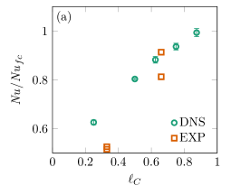
(a)

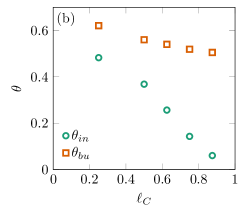
(b)

Figure 9: (a) Normalized Nusselt number $\mbox{{Nu}}/\mbox{{Nu}}_{fc}$ for various fraction $\ell_{C}$ of the conducting plate, while keeping the pattern frequency $f=9$, $\mbox{{Ra}}=10^{8}$, and $\mbox{{Pr}}=1$ (green circles), and the rectangular tank of Wang et al. (2017) (orange squares). (b) Average temperature just below the insulating area $\theta_{in}$ and average bulk temperature $\theta_{bu}$, both plotted against $\ell_{C}$. Other parameters are the same as for (a).

Figure 9b shows two different temperatures, namely, the average temperature just below the insulating region $\theta_{in}$ and the average bulk temperature $\theta_{bu}$ measured at mid-height of the system. For $\ell_{C}=0.85$, $\theta_{in}$ is very close to zero, i.e. the top wall temperature. This is consistent with Nu nearly having the value of the conducting case (figure 9a). Also the bulk temperature is very close to the fully conducting case $\theta=0.5$. When $\ell_{C}$ is decreased, making the top plate less and less conducting, $\theta_{in}$ increases gradually, reaching $\theta_{in}=0.5$ when $\ell_{C}=0.25$. This equals the bulk temperature in a fully conducting system. However, when $\ell_{C}$ is decreased, also the bulk temperature gradually increases and nearly reaches 0.6 for $\ell_{C}=0.25$. This rise in the bulk temperature is much slower than the rise in the temperature above the insulating area, meaning that the gradient between insulating regions at the plate and the bulk decreases and thus does the heat transfer, see figure 9a. Even though these simulations were conducted using only $f=9$, one expects similar trends to apply for other values of $f$. From the previous simulations we found that when increasing $f$, $\mbox{{Nu}}/\mbox{{Nu}}_{fc}$ will rise and $\Theta_{ins}$ will decrease. The same response can be achieved by increasing $\ell_{C}$ as we increase the conducting area and approach the case of the fully conducting system.

3.4 Mixed insulating and conducting patterns in two dimensions

Until now, all patterns that have been applied to the top and bottom boundary wall were one-dimensional stripe-like patterns. We only varied the width of the patches and the ratio between the insulating and conducting fractions. In this subsection we add an additional spatial dependence to these patterns to make them checkerboard-like:

$$\theta(\hat{x},\hat{y},\hat{z}=1) =0 \hat{x}\in\left[iL_{px},L_{px1}+iL_{px}\right],\hat{y}\in\left[jL_{py},L_{py1}+jL_{px}\right],i,j\in\mathbb{Z}$$ (5)

$$\partial_{z}\theta(\hat{x},\hat{y},\hat{z}=1) =0 \hat{x}\notin\left[iL_{px},L_{px1}+iL_{px}\right],\hat{y}\notin\left[jL_{py},L_{py1}+jL_{px}\right],i,j\in\mathbb{Z}$$

$$\theta(\hat{x},\hat{y},\hat{z}=0) =1 \forall\hat{x},\hat{y}.$$

A schematic of a set of four patches, two insulating and two conducting, is shown in Figure 10. The dimensions of both types of patches were kept equal, i.e. $L_{px1}=L_{py1}=L_{px2}=L_{py2}$, meaning $\ell_{c}=1/2$.

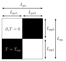
Figure 10: Top view of the top plate boundary conditions with applied checkerboard pattern ($f=1$). $L_{px}$ and $L_{py}$ are the horizontal and vertical dimensions of a set of patches. The set itself is divided in two insulating (white) and two conducting (black) areas, all with equal dimensions: $L_{px1}=L_{py1}=L_{px2}=L_{py2}$.

As we took both horizontal dimensions to be equal, we define a single frequency $f$ in both directions. The plate is divided in $f$ sets of patches which have dimensions $L_{px}=L_{py}=L_{p}$. When $f=1$ the complete boundary consists of a single set of patches. By increasing $f$ to 2, the plate will consist of four sets of four patches each. To give a further impression how the temperature fields resulting from these boundary conditions look like, two visualizations of instantaneous temperature fields for $f=4$ and $f=20$ are shown in Figure 11. The visualizations show respectively 16 and 400 sets of patches, which each consists of two insulating and two conducting areas.

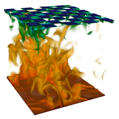
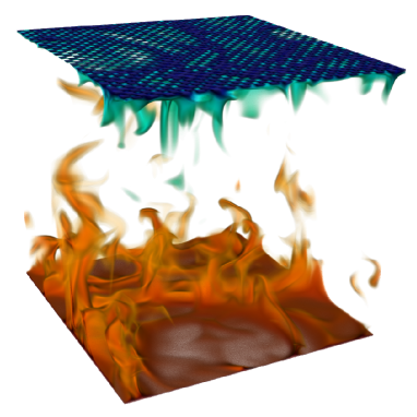
Figure 11: Two 3D visualizations of the instantaneous temperature field with different pattern frequencies at the top boundary. Hot fluid is shown in red while the cool fluid has a blue color. For both visualizations, $\mbox{{Ra}}=10^{8}$ and $\mbox{{Pr}}=1$. The left visualization shows $f=4$, which results in 16 sets of patches containing each two insulating patches and two conducting patches. The right visualization has $f=20$ which results in 400 sets of patches. Hot plumes rise from the bottom plate while cold plumes are ejected from the top boundary.

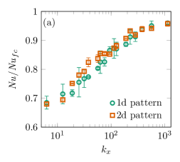
(a)

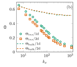
(b)

Figure 12: (a) Normalized Nusselt number $\mbox{{Nu}}/\mbox{{Nu}}_{fc}$ for 1D and 2D patterning versus $k_{x}$ for $\mbox{{Ra}}=10^{8}$ and $\mbox{{Pr}}=1$. The error bars show the statistical convergence error. (b) Average temperature $\theta_{in}$ just below the insulating area and average bulk temperature $\theta_{bu}$, both as function of $k_{x}$ for the 1D and 2D patternings. The Ra and Pr are the same as for (a).

Figure 12a shows the normalized Nusselt number $\mbox{{Nu}}/\mbox{{Nu}}_{fc}$ for the 1D- (stripe) and 2D (checkerboard) patterns as function of $k_{x}$. For these cases, $\mbox{{Ra}}=10^{8}$, $\mbox{{Pr}}=1$ and the error bars indicate the statistical convergence error. On first sight, the heat transfer is not that different when applying one-dimensional or two-dimensional patterning. At the lowest division, where we have divided the system into two or four areas for the 1D and 2D case respectively, the difference is negligible. Also at the highest value of $k_{x}$, the difference is inside statistical errors and seems insignificant.

On first glance, the 1D stripe pattern and the 2D checkerboard pattern may seem idealized representations. However, all other stripe and rectangular checkerboard patterns fall within these extreme cases, as the stripe pattern has $L_{px}/L_{py}\to\infty$ (or conversely $\to 0$), while for the checkerboard pattern $L_{px}/L_{py}=1$. Our work shows that, for the relatively small wavelengths considered here, the shape of these patterns do not have a significant influence on the flow dynamics. While we do not expect $\ell_{C}$ to considerably affect this statement, larger wavelength patterns could show some dependence on their shape. In the the experiments of Wang et al. (2017), the patches have wavelengths comparable to the system height and their distribution considerably affects the flow structure. Here, we consider wavelengths that are much smaller, affecting the flow only below the thermal boundary layer thickness, and reducing the Nusselt number. The largest wavelength considered in this work is still smaller than the smallest wavelength in the rectangular tank of Wang et al. (2017). There appear to be two clear regimes: the large patch regime, which show a clear influence on the flow dynamics and whose effect is likely to be shape-dependent, and the small patch regime, which only affect the boundary layers and thus the heat transfer. While there must exist a cross-over regime between both, it appears to be just outside the wavelengths we are considering.

When we look at $\theta_{in}$, the temperature just below the insulating region in Figure 12b, we see a similar trend. The temperature below the insulating region is on average always lower for the 2D pattern. This is even the case for the higher and lower limit of $k_{x}$. The average temperature just below the conducing area is very close to zero, regardless of which $k_{x}$. Therefore, the distance of the colder regions is shorter for the 2D- as for the 1D-pattern. This also explains that $\theta_{in}$ for the 2D case is slightly lower when compared to the 1D case. The bulk temperature for both the 1D and 2D cases are almost identical which means that the change in pattern has no effect on this quantity. From these results we can conclude that the impact of the two different patterns is very similar, and the quantitative differences between stripe and checkerboard patterns are at most small.

4 Summary and conclusions

A series of DNS of turbulent Rayleigh-Bénard convection using mixed conducting- and insulating boundary conditions were conducted. First, we applied a stripe-like pattern on the top boundary and varied the amount of stripes while keeping conduction-insulation ratio constant at $\ell_{C}=1/2$. When the top plate is divided in half, Nu has a value of approximately two-thirds of the fully conducting case. By increasing the frequency of the pattern, the Nu also increases, with a maximum value very close to as if it were fully conducting. With only half the effective conducting area on the top plate, when applying a dense pattern, the effect of the insulating patches almost completely vanishes. An increase in Ra results only in a marginal decrease in $\mbox{{Nu}}/\mbox{{Nu}}_{fc}$ for the largest $f$. This shift towards the fully conducting efficiency as seen with the Nusselt number when increasing the pattern frequency is also visible in $\theta_{bulk}$ and $\theta_{ins}$.

Using a two-dimensional Fourier transform, calculated from a horizontal slice of the instantaneous temperature it is possible to identify the imprint of the boundary conditions inside the flow. By comparing different spectra, each calculated from a horizontal slice slightly further away from the top boundary wall, the penetration depth of the boundary conditions inside the flow was investigated. The imprint of the striped pattern slowly fades away when moving from the top wall towards the border of the thermal boundary layer. Outside of the thermal boundary layer the imprint has completely vanished, even for the extreme case $f=1$. The thermal boundary layer masks the actual boundary, including all insulating imperfections and presents a new effective boundary to the bulk flow. In the thermal boundary layer, the heat is conducted to the conducting areas. This transport is more efficient when the pattern frequency is large. A lower Rayleigh number increases the thickness of the boundary layer and thereby, also increases the effectiveness of the heat transport.

Extending the pattern to both, the top and bottom boundary wall, resulted in similar behavior for the heat transfer and the average temperature below the insulating area. The primary difference is for the lowest pattern frequency where we practically have only half a RB cell and we find a Nusselt number with half the value of the fully conducting case. Adding an additional dimension to the pattern, creating a checkerboard-like pattern, also did not change the behavior significantly.

Our results demonstrate that small and even large imperfections in the temperature boundary conditions are barely felt in the system dynamics in terms of global heat transfer and local temperature measurements. Only in extreme cases as a half-and-half conducting and adiabatic plate was the effect significant. The effect of imperfect temperature boundary conditions of fully turbulent RB is weaker than the effects of velocity boundary conditions in two-dimensional RB (van der Poel et al., 2014), or the effect of rough elements near the boundaries (Tisserand et al., 2011). It is not yet clear if these boundary imperfections lead to significant changes in the dynamics of the bulk flow and this remains an open question for future works. Going beyond the scope of the present paper, we mention that the simulations by Cooper et al. (2013) and the experiments by Wang et al. (2017) show that with even larger adiabatic patches, changes in the flow topology can happen due to the arrangement of patches. The patches can also be varied in time, which is a way to control the bulk temperature or to fine tune the heat transfer, which is relevant for many industrial applications. In another work Whitehead & Behn (2015) showed that the combination of shear and mixed boundary conditions could also play a critical role in the system dynamics. Understanding the deeper reasons for this behavior may lead to better models for natural convection for geo- and astro-physically relevant flows.

Acknowledgments: We thank L. Biferale for his role in motivating this manuscript. We also thank V. Spandan, Y. Yang and X. Zhu for fruitful discussions. D.B. and E.P. were funded by FOM grants, and R.O. was funded by an ERC Advanced Grant. Computing time at the Dutch supercomputer Cartesius comes from a NWO grant.

Appendix A Numerical details

$\text{Ra}=10^{7}$,$\text{Pr}=1$, and $\ell_{c}=1/2$
$f$	Nu	$\Theta_{bulk}$	$\Theta^{top}_{ins}$
1	$11.82\pm 0.18$	0.67	0.69
2	$12.44\pm 0.31$	0.62	0.55
3	$12.75\pm 0.27$	0.61	0.48
4	$13.76\pm 0.01$	0.60	0.43
5	$13.86\pm 0.02$	0.59	0.40
9	$14.77\pm 0.07$	0.57	0.29
10	$14.56\pm 0.03$	0.57	0.28
12	$14.97\pm 0.15$	0.56	0.25
15	$14.81\pm 0.12$	0.55	0.22
18	$15.54\pm 0.15$	0.55	0.19
20	$15.68\pm 0.07$	0.55	0.18
30	$15.98\pm 0.15$	0.53	0.14
36	$16.02\pm 0.15$	0.53	0.12
45	$16.07\pm 0.14$	0.52	0.10
60	$16.60\pm 0.05$	0.52	0.08
90	$16.58\pm 0.15$	0.52	0.06
180	$16.95\pm 0.18$	0.51	0.05
fc	$16.90\pm 0.07$	0.50	–

$\text{Ra}=10^{8}$,$\text{Pr}=1$, and $\ell_{c}=1/2$
$f$	Nu	$\Theta_{bulk}$	$\Theta^{top}_{ins}$
1	$22.08\pm 0.72$	0.65	0.66
2	$23.04\pm 1.09$	0.61	0.57
3	$23.14\pm 0.37$	0.60	0.52
4	$24.34\pm 1.64$	0.58	0.49
5	$24.74\pm 0.98$	0.57	0.45
6	$24.94\pm 0.03$	0.57	0.42
9	$25.90\pm 0.10$	0.56	0.37
10	$26.59\pm 1.25$	0.56	0.36
12	$26.62\pm 0.46$	0.56	0.34
15	$27.90\pm 0.41$	0.55	0.30
18	$28.11\pm 1.09$	0.54	0.28
20	$28.06\pm 0.75$	0.54	0.26
30	$28.58\pm 0.24$	0.54	0.21
36	$29.39\pm 0.81$	0.53	0.19
45	$29.42\pm 0.53$	0.52	0.16
60	$30.23\pm 0.20$	0.53	0.14
90	$30.64\pm 0.53$	0.51	0.11
180	$30.95\pm 0.12$	0.51	0.09
fc	$32.87\pm 0.33$	0.50	–

$\text{Ra}=10^{8}$,$\text{Pr}=10$, and $\ell_{c}=1/2$
$f$	Nu	$\Theta_{bulk}$	$\Theta^{top}_{ins}$
1	$22.92\pm 0.18$	0.65	0.67
2	$24.04\pm 0.23$	0.62	0.58
3	$23.84\pm 0.11$	0.60	0.53
4	$24.86\pm 0.03$	0.59	0.50
5	$26.55\pm 0.88$	0.58	0.48
6	$25.32\pm 0.80$	0.58	0.46
9	$26.94\pm 0.18$	0.57	0.37
10	$26.71\pm 0.62$	0.57	0.37
12	$27.58\pm 0.40$	0.56	0.34
15	$27.79\pm 0.15$	0.55	0.31
18	$27.66\pm 0.28$	0.55	0.28
20	$28.80\pm 0.19$	0.55	0.26
30	$29.06\pm 0.09$	0.54	0.22
36	$28.96\pm 1.01$	0.54	0.2
45	$29.33\pm 0.17$	0.53	0.17
60	$30.27\pm 0.38$	0.53	0.14
90	$29.98\pm 1.10$	0.52	0.11
180	$30.60\pm 0.54$	0.52	0.08
fc	$32.63\pm 0.13$	0.50	–

$\text{Ra}=10^{9}$,$\text{Pr}=1$, and $\ell_{c}=1/2$
$f$	Nu	$\Theta_{bulk}$	$\Theta^{top}_{ins}$
1	$43.87\pm 0.22$	0.65	0.65
2	$45.05\pm 0.27$	0.62	0.60
3	$45.94\pm 0.19$	0.61	0.56
4	$47.14\pm 0.09$	0.60	0.53
5	$47.66\pm 0.28$	0.59	0.50
9	$49.15\pm 0.28$	0.58	0.44
10	$50.24\pm 1.41$	0.58	0.43
12	$51.46\pm 0.73$	0.57	0.41
15	$51.48\pm 0.05$	0.57	0.38
18	$52.87\pm 0.32$	0.56	0.36
20	$53.54\pm 0.97$	0.56	0.35
30	$54.84\pm 0.37$	0.55	0.30
36	$55.7\pm 0.03$	0.55	0.28
45	$55.71\pm 0.20$	0.54	0.26
60	$56.52\pm 0.92$	0.54	0.23
90	$58.36\pm 0.38$	0.53	0.20
180	$59.42\pm 0.68$	0.52	0.16
fc	$64.66\pm 0.33$	0.50	–

Table 1: Data from all numerical simulations for the single-sided mixed boundary conditions and the fully conducting case, used in figures 4a, 5a, 5b, and 8b. The ‘fc’ in the f column indicates the fully conducting case, e.g. without the striped pattern.

$\text{Ra}=10^{8}$,$\text{Pr}=1$, and $\ell_{c}=1/2$
$f$	Nu	$\Theta_{bulk}$	$\Theta^{top}_{ins}$	$\Theta^{bot}_{ins}$
1	$16.96\pm 0.11$	0.52	0.55	0.53
2	$17.67\pm 0.03$	0.52	0.56	0.49
4	$19.10\pm 0.33$	0.55	0.64	0.45
10	$21.98\pm 0.17$	0.53	0.71	0.34
15	$23.60\pm 0.39$	0.53	0.74	0.28
20	$24.77\pm 0.26$	0.52	0.78	0.25
36	$26.93\pm 0.42$	0.51	0.83	0.18
60	$27.76\pm 0.98$	0.50	0.87	0.14
90	$29.03\pm 0.33$	0.50	0.89	0.11
180	$30.10\pm 0.97$	0.51	0.92	0.08

Table 2: Data from all numerical simulations for the double sided mixed boundary conditions, used in figure 8a and 8b.

$\text{Ra}=10^{8}$,$\text{Pr}=1$, and $\ell_{c}=1/2$
$f$	Nu	$\Theta_{bulk}$	$\Theta^{top}_{ins}$
1	$22.35\pm 0.26$	0.64	0.61
2	$22.82\pm 0.21$	0.61	0.52
3	$24.69\pm 0.06$	0.60	0.46
4	$25.64\pm 0.19$	0.59	0.42
5	$26.06\pm 0.20$	0.58	0.39
6	$27.09\pm 0.51$	0.58	0.37
9	$27.51\pm 0.43$	0.56	0.30
10	$28.10\pm 0.02$	0.56	0.29
12	$28.06\pm 0.12$	0.56	0.26
15	$28.02\pm 0.03$	0.55	0.23
18	$28.71\pm 0.02$	0.55	0.21
20	$28.96\pm 0.32$	0.54	0.20
30	$29.81\pm 0.06$	0.53	0.16
36	$30.66\pm 0.01$	0.53	0.14
45	$30.20\pm 0.07$	0.53	0.12
60	$30.86\pm 0.31$	0.52	0.11
90	$30.95\pm 0.04$	0.52	0.08
180	$31.48\pm 0.28$	0.51	0.06

Table 3: Data from all numerical simulations of the checkerboard pattern used in figure 12a and 12b.

$\text{Pr}=1$, and $\ell_{c}=1/2$
$f$	Ra	Nu		$f$	Ra	Nu
1	$1\text{\times}{10}^{7}$	11.82		90	$1\text{\times}{10}^{9}$	58.36
1	$1\text{\times}{10}^{8}$	22.08		90	$3\text{\times}{10}^{9}$	81.37
1	$3\text{\times}{10}^{8}$	30.18		180	$1\text{\times}{10}^{7}$	16.95
1	$1\text{\times}{10}^{9}$	43.87		180	$1\text{\times}{10}^{8}$	30.95
1	$3\text{\times}{10}^{9}$	63.26		180	$3\text{\times}{10}^{8}$	42.43
10	$1\text{\times}{10}^{7}$	14.56		180	$1\text{\times}{10}^{9}$	59.42
10	$1\text{\times}{10}^{8}$	26.59		180	$3\text{\times}{10}^{9}$	82.53
10	$3\text{\times}{10}^{8}$	35.58		fc	$1\text{\times}{10}^{7}$	16.99
10	$1\text{\times}{10}^{9}$	50.24		fc	$1\text{\times}{10}^{8}$	32.87
10	$3\text{\times}{10}^{9}$	70.73		fc	$3\text{\times}{10}^{8}$	44.71
90	$1\text{\times}{10}^{7}$	16.58		fc	$1\text{\times}{10}^{9}$	63.95
90	$1\text{\times}{10}^{8}$	30.64		fc	$3\text{\times}{10}^{9}$	92.15
90	$3\text{\times}{10}^{8}$	41.34

Table 4: Nusselt and Rayleigh numbers for various $f$ and the fully conducting case, used in figure 3a and 3b

References

- Ahlers et al. (2009) Ahlers, G., Grossmann, S. & Lohse, D. 2009 Heat transfer and large scale dynamics in turbulent Rayleigh-Bénard convection. Rev. Mod. Phys. 81, 503–537.
- Cattaneo et al. (2003) Cattaneo, F., Emonet, T. & Weiss, N. 2003 On the interaction between convection and magnetic fields. Astrophys. J. 588, 1183–1198.
- Chillà & Schumacher (2012) Chillà, F. & Schumacher, J. 2012 New perspectives in turbulent Rayleigh-Bénard convection. Eur. Phys. J. E 35 (7).
- Cooper et al. (2013) Cooper, C. M., Moresi, L. N. & Lenardic, A. 2013 Effects of continental configuration on mantle heat loss. Geoph. Res. Lett. 40 (12), 2647–2651.
- Glatzmaier & Roberts (1995) Glatzmaier, G. A. & Roberts, P. H. 1995 A 3-dimensional self-consistent computer simulation of a geomagnetic field reversal. Nature 377, 203–209.
- Huang et al. (2015) Huang, S.-D., Wang, F., Xi, H.-D & Xia, K.-Q. 2015 Comparative experimental study of fixed temperature and fixed heat flux boundary conditions in turbulent thermal convection. Phys. Rev. Lett. 115, 154502.
- Jin & Xia (2008) Jin, X.-L. & Xia, K.-Q. 2008 An experimental study of kicked thermal turbulence. J. Fluid Mech. 606, 131–151.
- Johnston & Doering (2007) Johnston, H. & Doering, C. R. 2007 Rayleigh-Bénard convection with imposed heat flux. Chaos 17, 041103.
- Johnston & Doering (2009) Johnston, H. & Doering, C. R. 2009 Comparison of turbulent thermal convection between conditions of constant temperature and constant flux. Phys. Rev. Lett. 102, 064501.
- Kelly & Pal (1978) Kelly, R. E. & Pal, D. 1978 Thermal convection with spatially periodic boundary conditions:resonant wavelength excitation. J. Fluid Mech. 86, 433–456.
- Lenardic et al. (2005) Lenardic, A., Moresi, L. N., Jellinek, M. A. & Manga, M. 2005 Continental insulation, mantle cooling and the surface area of oceans and continents. Earth and Planetary Science Letters 234, 317–333.
- Lohse & Xia (2010) Lohse, D. & Xia, K.-Q. 2010 Small-scale properties of turbulent Rayleigh-Bénard convection. Ann. Rev. Fluid Mech. 42, 335–364.
- Marcq & Weiss (2012) Marcq, S. & Weiss, J. 2012 Influence of sea ice lead-width distribution on turbulent heat transfer between the ocean and the atmosphere. Cryosphere 6, 143–156.
- Marshall & Schott (1999) Marshall, J. & Schott, F. 1999 Open-ocean convection: Observations, theory, and models. Rev. Geophys. 37, 1–64.
- McKenzie et al. (1974) McKenzie, D. P., Roberts, J. M. & Weiss, N. O. 1974 Convection in the Earth’s mantle: towards a numerical simulation. J. Fluid Mech. 62, 465–538.
- Normand et al. (1977) Normand, C., Pomeau, Y. & Velarde, M. H. 1977 Convective instability: a physicist’s approach. Rev. Mod. Phy. 49, 465–538.
- van der Poel et al. (2015) van der Poel, E. P., Ostilla-Monico, R., Donners, J. & Verzicco, R. 2015 A pencil distributed finite difference code for strongly turbulent wall-bounded flows. Comp. Fluids 116, 10–16.
- van der Poel et al. (2014) van der Poel, E. P., Ostilla-Mónico, R., Verzicco, R. & Lohse, D. 2014 Effect of velocity boundary conditions on the heat transfer and flow topology in two-dimensional rayleigh-bénard convection. Phys. Rev. E 90, 013017.
- Ripesi et al. (2014) Ripesi, P., Bigerale, L., Sbragaglia, M. & Wirth, A. 2014 Natural convection with mixed insulating and conducting boundary conditions: low- and high-rayleigh-number regimes. J. Fluid Mech. 742, 636–663.
- Shraiman & Siggia (1990) Shraiman, B. I. & Siggia, E. D. 1990 Heat transport in high-Rayleigh number convection. Phys. Rev. A 42, 3650–3653.
- Spiegel (1971) Spiegel, E. A. 1971 Convection in stars. Ann. Rev. Astron. Astrophys. 9, 323–352.
- Stevens et al. (2011) Stevens, R. J. A. M., Lohse, D. & Verzicco, R. 2011 Prandtl and Rayleigh number dependence of heat transport in high Rayleigh number thermal convection. J. Fluid Mech. 688, 31–43.
- Stevens et al. (2010) Stevens, R. J. A. M., Verzicco, R. & Lohse, D. 2010 Radial boundary layer structure and Nusselt number in Rayleigh-Bénard convection. J. Fluid Mech. 643, 495–507.
- Tisserand et al. (2011) Tisserand, J. C., Creyssels, M., Gasteuil, Y., Pabiou, H., Gibert, M., Castating, B. & Chilla, F. 2011 Comparison between rough and smooth plates within the same Rayleigh-Bénard cell. Phys. Fluids 23, 015105.
- Verzicco (2004) Verzicco, R. 2004 Effect of non-perfect thermal sources in turbulent thermal convection. Phys. Fluids 16, 1965–1979.
- Verzicco & Orlandi (1996) Verzicco, R. & Orlandi, P. 1996 A finite-difference scheme for three-dimensional incompressible flow in cylindrical coordinates. J. Comput. Phys. 123, 402–413.
- Wang et al. (2017) Wang, F., Huang, S.-D. & Xia, K.-Q. 2017 Thermal convection with mixed thermal boundary conditions: Effects of insulating lids at the top. J. Fluid Mech. in press (2017), arXiv 1702.04105.
- Whitehead & Behn (2015) Whitehead, J. A. & Behn, M. D. 2015 The continental drift convection cell. Geoph. Res. Lett. 42 (12), 2015GL064480.
- Wirth & Barnier (2006) Wirth, A. & Barnier, B. 2006 Tilted convective plumes in numerical experiments. Ocean Modelling 12, 101–111.
- Yoo & Moon (1991) Yoo, J. S. & Moon, U. 1991 Two-dimensional convection in a horizontal fluid layer with spatially periodic boundary temperatures. Fluid Dyn. Res. 7, 181–200.
- Zhao et al. (2014) Zhao, L., Lee, X., Smith, R. B. & Oleson, K. 2014 Strong contributions of local background climate to urban heat islands. Nature 511, 216–219.