Resource Sharing Among mmWave Cellular Service Providers in a Vertically Differentiated Duopoly

Abstract

With the increasing interest in the use of millimeter wave bands for 5G cellular systems comes renewed interest in resource sharing. Properties of millimeter wave bands such as massive bandwidth, highly directional antennas, high penetration loss, and susceptibility to shadowing, suggest technical advantages to spectrum and infrastructure sharing in millimeter wave cellular networks. However, technical advantages do not necessarily translate to increased profit for service providers, or increased consumer surplus. In this paper, detailed network simulations are used to better understand the economic implications of resource sharing in a vertically differentiated duopoly market for cellular service. The results suggest that resource sharing is less often profitable for millimeter wave service providers compared to microwave cellular service providers, and does not necessarily increase consumer surplus.

I Introduction

With the introduction of millimeter wave (mmWave) cellular systems as a candidate for the next generation of mobile networks, there has been renewed interest in problems related to sharing resources, i.e. spectrum and base stations (BSs). Early results suggest that compared to conventional microwave frequencies, the massive bandwidth, increased spatial degrees of freedom, and greater path loss increase the technical benefits of resource sharing in mmWave frequencies [1, 2, 3, 4]. Some have suggested that these technical gains will translate to economic gains. For example, [1] claims that it is economical for mmWave service providers to share resources because they can offer the same quality of service while licensing less spectrum. Similarly, [4] considers a scenario where a primary mmWave spectrum holder can earn additional revenue by licensing the spectrum in a secondary market with the condition of restricted interference to its own users. However, even if service providers can reduce licensing costs or earn revenue from secondary licensing while keeping quality of service the same, resource sharing can affect profits if it shifts demand to a competing service provider, or if it changes the market dynamics in a way that forces down the price. None of [1, 2, 3, 4] consider the effects of demand and competition.

Some of the literature in both engineering and economics disciplines addresses economic and regulatory aspects of resource sharing in conventional cellular networks [5, 6, 7, 8, 9]. However, the fundamental technical differences between mmWave and microwave frequencies also affect the markets for these services. For example, an early economic perspective on mmWave networks [10] suggests that their limited coverage range is a key challenge for their cost efficiency. Similarly, our previous work [11] shows that the dynamics of demand and ease of market entry, and the effect of unlicensed spectrum or open association small cells on these, are different in mmWave networks (compared to microwave small cell networks). Thus, we posit that the economic impact of resource sharing may also be different. To gain a fuller understanding of the benefits of resource sharing in mmWave networks, we need to identify the specific impact on quality of service, and then understand how this affects the demand, price, and cost of service.

The goal of this work, therefore, is to understand the strategic decisions of wireless service providers with respect to resource sharing in mmWave 5G cellular networks. We apply the economic model of compatibility of network goods [12, 13] to resource sharing in mmWave cellular networks. We describe a duopoly game involving two vertically differentiated cellular service providers, and compare mmWave and microwave networks with respect to service provider profits, market coverage, consumer surplus, and price of service with and without resource sharing.

The rest of this paper is organized as follows. We begin with a brief introduction to the economic framework used in this paper, in Section II. In Section III, we describe the wireless system model, and show simulation results in Section IV. In Section V, we describe a duopoly game involving two vertically differentiated network service providers, and compare the benefits of resource sharing decisions to consumers and service providers in mmWave and microwave networks. Finally, in Section VI, we conclude with a discussion of the implications of this work and areas of further research.

II Economic foundations

In this paper, we use an economic model that includes several important considerations for resource sharing in cellular networks:

• Network effect. This captures the effect of a large network service provider (NSP) with more subscribers typically having more base stations and spectrum than a competitor with a smaller market share.

• Compatibility. This models the decision of an NSP to share resources (base stations and spectrum) and potentially increase the value of its service to subscribers, or to preserve its own market power by not sharing resources.

• Vertical differentiation. This models the ability of an NSP to distinguish itself from competitors in aspects of its service other than network size and price.

The network size and the extent of the network effect, as well as the compatibility (resource sharing) decision, determine the consumer’s expected data rate, and the vertical differentiation captures other factors affecting consumers’ decisions such as customer service and availability of desirable handsets.

In economics, a network good or service [14] is a product for which the utility that a consumer gains from the product varies with the number of other consumers of the product (the size of the network). This effect on utility - which is called the network externality or the network effect - may be direct or indirect. For example, consumers of a telephone network, which is more valuable when the service has more subscribers, benefit from a direct network effect. The classic example of an indirect effect is the hardware-software model, e.g. a consumer who purchases an Android smartphone will benefit if other consumers also purchase Android smartphones, because this will incentivize the development of new and varied applications for the Android platform. The network externality may also be negative, for example, if an Internet service provider becomes oversubscribed, its subscribers will suffer from the congestion externality. Network effects and the standard models for understanding them have been empirically validated in a variety of industries, including the markets for mobile phones [15], fixed broadband [16], personal digital assistants [17], DVDs [18], home video games [19], ATMs [20], and fax machines [21].

Consider a set of consumers in a market for a good. Total demand for the good, $n$, is normalized so that $n=1$ when all consumers purchase the good, and $n=0$ when no consumers purchase the good. Heterogeneous consumers are parameterized by the “taste parameter” $\omega$, $0\leq\omega\leq\hat{\omega}$. A consumer with a high $\omega$ is willing to pay more for a high-quality good.

In the case of a non-network good, the utility of a consumer of type $\omega$ may be modeled as $u(\omega,p)=\omega-p$, and the consumer is indifferent between purchasing the good or not when price $p=\omega$. For $p>\hat{\omega}$, no consumer will purchase the good ($n=0$), because it is too expensive even for consumers with the highest value of $\omega$. At $p=0$, all of the consumers will purchase the good ($n=1$). The demand curve, which indicates what portion of the consumers will purchase the good at a given price, has a negative slope for most non-network goods, because the quantity demanded $n$ increases as the price of the good $p$ decreases. Conversely, to increase demand for a typical non-network good, the producer must reduce its price.

In the case of a network good, a consumer of type $\omega$ purchasing the good at price $p$ gains utility $u(\omega,n,p)=\omega h(n)-p$, where $n$ is the network size, and $h(n)$ is a network externalities function indicating how consumer utility scales with $n$. For a positive network externality, $h(n)$ increases with $n$, and for a negative network externality $h(n)$ decreases with $n$. With a positive network externality, the demand curve may have a positive slope. Unlike a non-network good, where increasing the price reduces the demand for the good, the value of a network good varies with the number of consumers, so as more units are sold, the value increases and the producer can raise the price. For a more detailed overview, see [14].

Producers of a network good with a positive network externality therefore prefer to increase the size of their network. In addition to selling more units of the good, producers may increase network size by making compatible goods [12, 13]. When two network goods are compatible, then the total network effect for a consumer of either good is based on the sum network size of both goods. In other words, the network externalities function for good $i$ is evaluated using the total network size for all the goods: $h(\sum_{j\in I}n_{j})$, where $I$ is a set of firms producing compatible goods and $i\in I$. Then the utility of a consumer of type $\omega$ purchasing good $i$ at price $p$ is $u(\omega,\sum_{j\in I}n_{j},p)=\omega h(\sum_{j\in I}n_{j})-p$, $i\in I$. A producer of a network good with a positive network externality has incentives for and against compatibility:

• Network effect: A compatible product is more valuable to consumers, since the argument to $h(\cdot)$ is greater.

• Market power: Making a product compatible increases the value of a competitors’ product and reduces the perceived difference between competing products, potentially increasing price competition and forcing prices down. Price competition occurs when competing products are very similar, so consumers’ purchasing decisions are made mainly on the basis of which is cheaper.

Compatibility is often used to model a firm’s choice to use a proprietary technical standard or a common industry standard. For example, the developers of a word processing application might choose to use a proprietary file format so that all consumers who need to open these files must purchase their software, or they might choose to use an open standard so that their users can share the files produced with their software with users of other word processors.

The effect of the latter issue, loss of market power, is partially mitigated by vertical differentiation. With vertical differentiation, a producer may choose compatibility and still distinguish itself from competitors and reduce price competition by improving the quality of its good in other ways (not by increasing $n$). For example, consumers of Android-based smartphones benefit from the network effects due to consumers of all Android-compatible smartphones. However, a producer of Android phones can distinguish itself by selling handsets with better hardware specifications than its competitors’. With vertical differentiation, different providers capture different portions of the market (e.g., low end vs. high end).

In this paper, we use a model of consumer utility in a market for network goods with vertical differentiation, described in [22]. The willingness to pay of a consumer of type $\omega$ for good $i$ is $\omega q_{i}+q_{i}h(\sum_{j\in I}n_{j})$, where $I$ is a set of firms producing compatible goods, $i\in I$, and $q_{i}$ is a scaling factor that represents aspects of the good’s quality that are not a function of the network size. Firms that produce compatible goods can distinguish themselves from one another by choosing different quality levels. However, a firm that produces a higher-quality good also has higher marginal costs; the marginal cost to the producer of producing one unit of good $i$ is $q_{i}$, its total cost is $c(q_{i},n_{i})=q_{i}n_{i}$, and its profits are then $\pi_{i}(q_{i},n_{i},p_{i})=n_{i}p_{i}-q_{i}n_{i}$.

Given this economic framework, we are interested in modeling mmWave network service as a network good, to better understand the conditions under which mmWave network service providers will want to share resources, and whether or not it is desirable for a regulator to enforce resource sharing. To answer these questions, however, we must characterize $h(n)$, the function that determines the network effect. In the next section, we describe the simulation from which we empirically derive $h(n)$ for mmWave and microwave small cell networks.

III System Model

We describe the system model of the mmWave and microwave network simulations. The results of this simulation will be used to parameterize the economic model for resource sharing. Our simulation captures the following key characteristics of mmWave and small cell microwave networks:

• Channel model: We use the empirically derived line of sight (LOS), NLOS and outage probabilistic channel models for mmWave links from [23]. For the microwave links, we use the microcell channel model described in [24].

• Directional transmission: We use the antenna pattern model described in [25]. For mmWave frequencies we use model parameters representing an 8x8 antenna array at the base station (BS) and a 4x4 antenna array at the user equipment (UE). For microwave frequencies, we use the ITU model for the BS antenna [24], and an omnidirectional UE antenna.

We consider a system with two NSPs. NSP $i\in\{1,\dots,I\}$ has bandwidth $W_{i}$, BSs distributed in the network area using a homogeneous Poisson Point Process (hPPP) with intensity $\lambda^{B}_{i}$, and UEs whose locations are modeled by an independent hPPP with intensity $\lambda^{U}_{i}$.

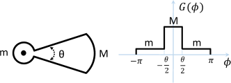
Both BSs and UEs may use antenna arrays for directional beamforming. We approximate the actual array patterns using a simplified pattern as in [25, 26]. Let $G(\phi)$ denote the simplified antenna directivity pattern depicted in Fig. 1, where $M$ is the main lobe power gain, $m$ is the back lobe gain and $\theta$ is the beamwidth of the main lobe. In general, $m$ and $M$ are proportional to the number of antennas in the array and $M/m$ depends on the type of the array. Furthermore, $\theta$ is inversely proportional to the number of antennas, i.e., the greater the number of antennas, the more beam directionality. We let $G^{B}(\phi)$ (which is parameterized by $M^{B}$, $m^{B}$, and $\theta^{B}$) be the antenna pattern of the BS, and $G^{U}(\phi)$ (which is parameterized by $M^{U}$, $m^{U}$, and $\theta^{U}$) be the antenna pattern of the UE.

Figure 1: Simplified antenna pattern with main lobe $M$, back lobe $m$ and beamwidth $\theta$.

We model a time-slotted downlink of a cellular system. For path loss, shadowing, and outage, line of sight (LOS), and NLOS probability distributions, we use models adopted from [23] and [24] for mmWave and microwave links, respectively. We assume Rayleigh block fading. The data rate is modeled as

$$R=(1-\alpha)W\log_{2}\Bigg{(}1+\beta\frac{PG^{U}(0)G^{B}(0)H}{N_{f}N_{0}W+I}\Bigg{)},$$ (1)

where $\alpha$ and $\beta$ are overhead and loss factors, respectively, and are introduced to fit a specific physical layer to the Shannon capacity curve [27]. Furthermore, $P$ is the BS transmitting power, and $H$ is the channel power gain derived from the model discussed above, incorporating the effects of fading, shadowing, outage, and path loss. We assume perfect beam alignment between BS and UE within a cell, therefore the antenna power gain (link directionality) is $G^{U}(0)G^{B}(0)=M^{U}M^{B}$. Finally, $N_{f}$, $N_{0}$, $W$ and $I$ are UE noise figure, noise power spectral density, bandwidth, and interference power, respectively.

In the mmWave scenario, each cell belonging to a given NSP $i$ reuses the whole bandwidth $W_{i}$ available to that NSP, with no coordination between cells. Although it is possible to have strong interference due to the lack of coordination, the narrow beamwidth, increased channel loss, and large bandwidth (hence large noise power) in the mmWave scenario mean that noise and not interference is usually the dominant effect [23]. In the microwave scenario, where intercell interference is stronger, we use frequency reuse as in [28]. For frequency reuse factor $\delta$, each cell is randomly assigned one band with bandwidth $\frac{W_{i}}{\delta}$ from the $\delta$ bands available to each NSP.

Early work on resource sharing in mmWave networks [1, 3, 29, 2] has focused on signal propagation and interference effects in networks with shared resources. To approximate the data rate at a UE, they divide its link capacity as determined by SINR by the total number of UEs in the cell. In a realistic network with opportunistic scheduling, however, a UE may achieve a higher data rate than its average SINR would suggest, because it is scheduled with higher priority in time slots when its SINR is high. For an economic analysis we need to accurately model how consumers’ utility scales with all aspects of network size, including the number of subscribers, so our model must include this scheduling gain. We adopt a modified scheduler based on the multicell temporal fair opportunistic scheduler proposed in [30]. That scheduler involves two stages: in the first stage a UE is nominated for each cell, and then, after some coordination among base stations, a subset of the nominated users are scheduled in the second stage. We have no coordination between BSs, so we use only the first (user nomination) stage of the scheduler mentioned above. Thus each BS runs the scheduler and selects a UE independently, without considering intercell interference.

IV Network simulation results

Using the model of Section III, we simulate mmWave and microwave networks with the parameters given in Table I.

TABLE I: Network parameters

Parameter	mmWave	microwave
Frequency	73 GHz	2.5 GHz
Max. bandwidth ($W_{\text{max}}$)	1 GHz	300 MHz
Frequency reuse factor	1	3
Max. BS density ($\lambda^{B}_{\text{max}}$)	100 BSs/$\text{km}^{2}$	100 BSs/$\text{km}^{2}$
Max. UE density ($\lambda^{U}_{\text{max}}$)	500 UEs/$\text{km}^{2}$	500 UEs/$\text{km}^{2}$
BS transmit power $P$	30 dBm	30 dBm
($M^{B}$,$m^{B}$,$\theta^{B}$)	(20 dB, -10 dB, 5°)	(0 dB, -20 dB, 70°)
($M^{U}$,$m^{U}$,$\theta^{U}$)	(10 dB, -10 dB, 30°)	(0 dB, 0 dB, 360°)
Simulation area	1 $\text{km}^{2}$	1 $\text{km}^{2}$
Rate model ($\alpha$, $\beta$)	(0.2, 0.5)	(0.2, 0.5)
UE noise figure $N_{f}$	7 dB	7 dB
Noise PSD $N_{0}$	-174 dBm/Hz	-174 dBm/Hz

Recall that we model mmWave network service as a network good, as described in Section II. Subscribers benefit from an indirect positive network externality: a large NSP with more subscribers (higher density of UEs) will build a denser deployment of BSs and purchase more spectrum. Thus network size of NSP $i$, $n_{i}$, represents the normalized demand for the service (scaled to the range $[0,1]$), but is also a scaling factor on the BS density and bandwidth of the NSP. Specifically, as $n_{i}$ varies, the UE density $\lambda_{i}^{U}$ is $n_{i}\lambda_{\text{max}}^{U}$, the BS density $\lambda_{i}^{B}$ is $n_{i}\lambda_{\text{max}}^{B}$, and the bandwidth $W_{i}$ is $n_{i}W_{\text{max}}$. We then find the net effect of increasing network size $n_{i}$ on subscribers’ fifth percentile data rates. We use fifth percentile rates as a key metric of utility because research on human behavior suggests that service reliability is rated highly in perceived quality of mobile service [31]. We take the fifth percentile rate as a proxy for service reliability to obtain $h(n)$, the network externalities function introduced in Section II.

(a)

(b)

Figure 2: Effect of increasing network size on fifth percentile data rates (used as a metric of consumer utility), with the piecewise line estimated by an ordinary least squares linear regression. Error bars show 95% bootstrap confidence intervals.

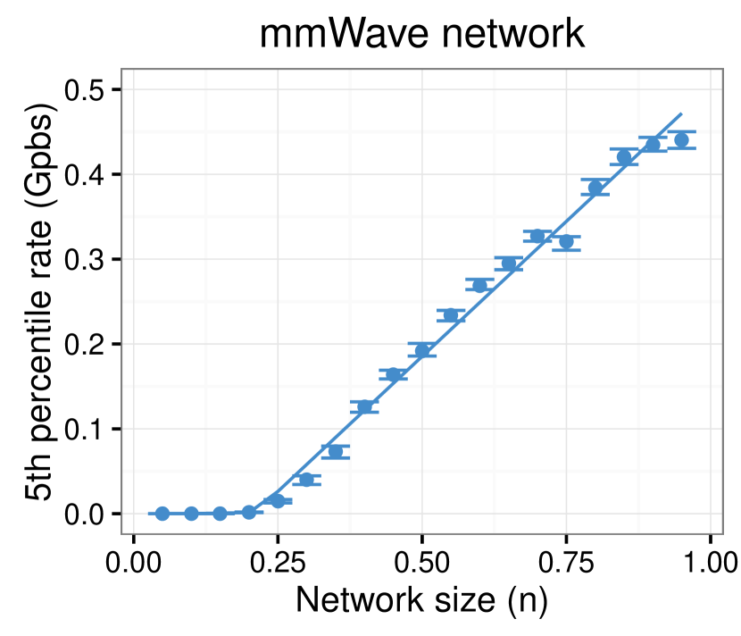
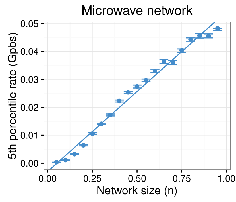
The simulation results are shown in Fig. 2. We approximate the variation of the fifth percentile rate with network size as a linear or piecewise linear relationship, estimated by an ordinary least squares linear regression, with breakpoints found using the segmented package for R [32].

We note two key differences between mmWave and microwave networks. First, in microwave networks, the fifth percentile rate increases beginning from a very small network size. In mmWave networks, the fifth percentile rate remains flat at first and starts increasing only at a moderate network size. This is due to the increased path loss at mmWave frequencies, where a denser deployment of BSs is necessary to prevent outage. Second, we note that for moderate or large networks, the network effect is stronger in mmWave networks, as per the slope of the line in Fig. 2(a) relative to the line in Fig. 2(b) (note the different vertical axis scales). This is due to the much larger bandwidth and the greater benefit due to having a LOS link in a mmWave network.

Fig. 2 also suggests some intuition regarding incentives for sharing in mmWave and microwave networks. The effect of resource sharing is similar to an increase in network size: when two NSPs of size $n_{1}$ and $n_{2}$ agree to share resources, subscribers of both NSPs experience the network effects due to the total network size $n_{1}+n_{2}$. Fig. 2 shows that network effect in mmWave networks is different, and that the network size has a greater impact on utility than in microwave networks. Thus resource sharing may be less profitable for a dominant (large $n$) mmWave service provider, because the advantage gained by its competitor due to sharing is greater than it would be in an equivalent microwave network scenario. In the next section, we will examine this intuition in the context of a duopoly game.

V Duopoly game

We model the NSPs’ decision to share network resources or not as a compatibility problem (introduced in Section II), where NSPs are considered compatible if their subscribers can connect to any of the set of NSPs’ BSs, and use a bandwidth equal to their pooled spectrum holdings. In many locations in the United States and around the world, the market for cellular service is effectively a duopoly. We therefore consider a market with two vertically differentiated NSPs, and the three-stage game with complete information described in [22]:

1. NSPs $i\in\{1,2\}$ simultaneously choose quality $q_{i}$ from $[0,\hat{q}]$.

2. NSPs $i\in\{1,2\}$ simultaneously set price $p_{i}$.

3. Each consumer subscribes to one NSP $i\in\{1,2\}$ or neither.

The quality $q_{i}$ is the inherent quality (with maximum feasible value $\hat{q}$). It refers to aspects of service unrelated to the size of the network, such as the quality of the legacy data network, customer service, and the availability of desirable handsets.

An NSP’s marginal costs are increasing in $q_{i}$, with cost function $c(q_{i},n_{i})=q_{i}n_{i}$, and so each NSP $i\in\{1,2\}$ seeks to maximize its profits

$$\pi_{i}(q_{i},n_{i},p_{i})=n_{i}p_{i}-q_{i}n_{i}$$ (2)

Consumers evaluate competing services in terms of the difference in their inherent qualities as well as their network externalities. We have heterogeneous consumers parameterized by $\omega$, with $\omega$ distributed uniformly from $[0,\hat{\omega}]$. The surplus of a consumer of type $\omega$ subscribing to NSP $i$ is given by

$$u(\omega,q_{i},\tilde{n}_{i},p_{i})=\omega q_{i}+q_{i}h(\tilde{n})-p_{i}$$ (3)

with $i\in\{1,2\}$, and each consumer subscribes to at most one NSP. If the NSPs share their mmWave network resources, then $\tilde{n}_{i}=\sum_{i\in\{1,2\}}n_{i}$, otherwise $\tilde{n}_{i}=n_{i}$.

The fifth percentile rate is linear or piecewise linear in the network size in a mmWave (Fig. 2(a)) or microwave network (Fig. 2(b)). We consider only moderate- to large-sized networks, corresponding to the line on the right side of Fig. 2(a). Thus the network externalities function $h(\tilde{n}_{i})$ is approximately linear in $\tilde{n}_{i}$, and we take $h(\tilde{n}_{i})=\mu\tilde{n}_{i}$ The scaling factor $\mu$ determines the intensity of the network externality, and is derived from slopes of the lines in Fig. 2 as $\mu_{mm}=0.64$ and $\mu_{\text{micro}}=0.05$.

(a) NSP profit, $\hat{q}=1$

(b) Price, $\hat{q}=1$

(c) Consumer surplus, $\hat{q}=1$

(d) Market share, $\hat{q}=1$

(e) NSP profit, $\hat{q}=1.5$

(f) Price, $\hat{q}=1.5$

(g) Consumer surplus, $\hat{q}=1.5$

(h) Market share, $\hat{q}=1.5$

Figure 3: Profit of each NSP, price set by NSP, total consumer surplus, and market share of each NSP (and total market coverage) in the duopoly game. As $\hat{\omega}$ increases, the market is more easily separated into high-end and low-end groups and NSPs compete primarily on quality, so there is less price competition. A similar effect occurs as $\hat{q}$ increases. The intensity of the network effect is $\mu_{mm}=0.64$ for mmWave networks and $\mu_{\text{micro}}=0.05$ for microwave networks.

By their choice of quality level, the NSPs segment the market into a low-end group (small-$\omega$ type) and a high-end group (large-$\omega$ type). Without loss of generality, we assign index 1 to the NSP that chooses the higher quality, i.e., $q_{1}>q_{2}$, and subscribers of NSP 1 belong to the large-$\omega$ group. We define two marginal consumers: the consumer of type $\underline{\omega}$ is indifferent between choosing no subscription and subscribing to NSP 2, and the consumer of type $\overline{\omega}$ is indifferent between subscribing to NSP 1 and subscribing to NSP 2.

Then the utility of the marginal consumer of type $\overline{\omega}$ satisfies

$$\overline{\omega}q_{1}+\mu q_{1}\tilde{n}_{1}-p_{1}=\overline{\omega}q_{2}+\mu q_{2}\tilde{n}_{2}-p_{2}$$ (4)

and the utility of the marginal consumer of type $\underline{\omega}$ satisfies

$$\underline{\omega}q_{2}+\mu q_{2}\tilde{n}_{2}-p_{2}=0$$ (5)

Also, the marginal consumer of type $\overline{\omega}$ defines the market share of the high-end service

$$n_{1}=\frac{\hat{\omega}-\overline{\omega}}{\hat{\omega}}$$ (6)

and the marginal consumers together define the market share of the low-end service

$$n_{2}=\frac{\overline{\omega}-\underline{\omega}}{\hat{\omega}}$$ (7)

We can solve (4)-(7) for $n_{1}$, $n_{2}$, $\overline{\omega}$, and $\underline{\omega}$, and thus determine the decisions of the consumers and the market share of each NSP given $p_{i},q_{i},i\in\{1,2\}$.

It is shown in [22] that when $0\leq\mu<\text{min}[1,\hat{\omega}/2]$ and the ratio of quality levels satisfies

$$\frac{q_{1}}{q_{2}}>\Bigg{(}\frac{\hat{\omega}^{2}}{(\hat{\omega}-\mu)(\hat{\omega}-2\mu)}\Bigg{)}$$ (8)

there is a unique Nash equilibrium with both NSPs’ prices higher than their marginal costs. Furthermore, if (4)-(7) satisfies

$$0<\underline{\omega}<\overline{\omega}<\hat{\omega}$$ (9)

then both NSPs have market share greater than zero. When both (8) and (9) hold, then there is a unique Nash equilibrium in which both NSPs earn non-zero profit. We are primarily interested in the scenario in which both service providers offer service at a non-zero profit, so we restrict our attention to these circumstances.

If (8) and (9) hold and NSPs do not share resources, then per [22] their equilibrium quality levels $q_{1,NS}^{*},q_{2,NS}^{*}$ are:

$$q_{1,NS}^{*}=\hat{q}$$ (10)

$$q_{2,NS}^{*}=\frac{\hat{q}(\hat{\omega}-\mu)^{2}\Big{[}11\hat{\omega}-10\mu-\sqrt{3(3\hat{\omega}^{2}+28\hat{\omega}\mu-20\mu^{2})}\Big{]}}{2\hat{\omega}^{2}(7\hat{\omega}-5\mu)}<\hat{q}$$ (11)

and their equilibrium prices $p_{1,NS}^{*},p_{2,NS}^{*}$ are:

The profits of the high-end NSP always increase with $q_{1}$, so it will use $\hat{q}$. The low-end NSP balances two competing effects: at high values of $q_{2}$ it captures more of the market, but is also more similar to $q_{1}$, which increases price competition.

The total consumer surplus is then

If the NSPs share resources, then per [22] their equilibrium quality levels $q_{1,S}^{*},q_{2,S}^{*}$ are:

$${}q_{1,S}^{*}=\hat{q}$$ (15)

$$q_{2,S}^{*}=\frac{\hat{q}(4\hat{\omega}-3\mu)}{7\hat{\omega}-6\mu}<\hat{q}$$ (16)

and their equilibrium prices $p_{1,S}^{*},p_{2,S}^{*}$ are:

$$p_{1,S}^{*}=q_{1}\Bigg{[}1+\frac{2\hat{\omega}(\hat{\omega}-1)(q_{1}-q_{2})}{(4\hat{\omega}-3\mu)q_{1}-\hat{\omega}q_{2}}\Bigg{]}>q_{1}$$ (17)

$$p_{2,S}^{*}=q_{2}\Bigg{[}1+\frac{\hat{\omega}(\hat{\omega}-1)(q_{1}-q_{2})}{(4\hat{\omega}-3\mu)q_{1}-\hat{\omega}q_{2}}\Bigg{]}>q_{2}$$ (18)

The total consumer surplus is then

We are also interested in the monopoly case, for comparison. When there is one NSP, the marginal consumer is defined by

$$\overline{\omega}q_{1}+\mu q_{1}\tilde{n}_{1}-p_{1}=0$$ (20)

and the market share of the NSP is

$$n_{1}=\frac{\hat{\omega}-\overline{\omega}}{\hat{\omega}}$$ (21)

At equilibrium, the monopoly NSP will choose quality level

$$q_{1,M}^{*}=\hat{q}$$ (22)

and price

$$p_{1,M}^{*}=\frac{q_{1}(\hat{\omega}-1)}{2}$$ (23)

The total consumer surplus is then

$$\int_{\overline{\omega}}^{\hat{\omega}}u(\omega,q_{1,M}^{*},n_{1},p_{1,M}^{*})\;d\omega$$ (24)

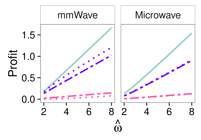
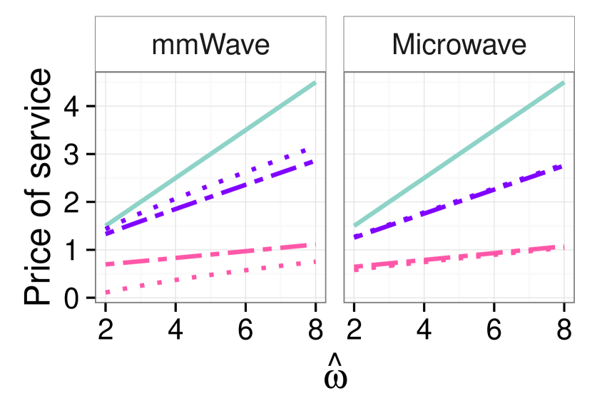
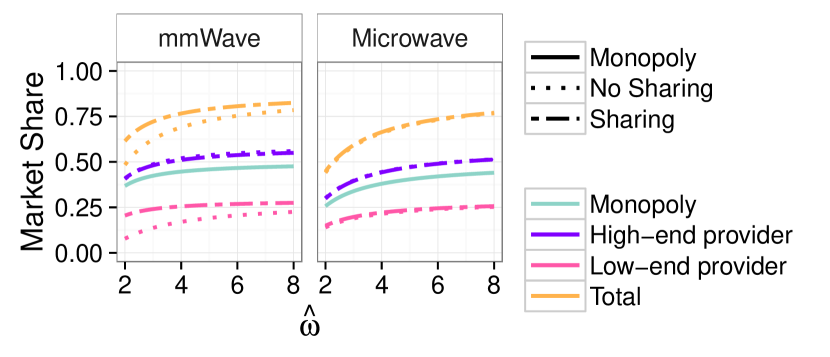
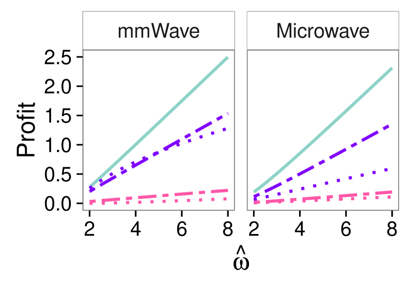
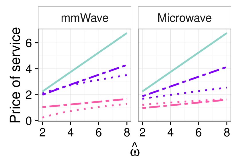
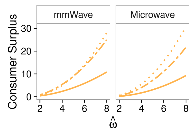
Fig. 3 shows the NSP profit (2); price (12), (13), (17), (18), and (23); total consumer surplus (14), (19), and (24); and market share (6), (7), and (21) in the duopoly game, for various market parameters ($\hat{\omega}$, $\hat{q}$). First, we note that our intuition of Section IV is validated: Fig. 3(a) and Fig. 3(e) show that resource sharing is less often profitable to both NSPs at the same time in mmWave networks than in microwave networks. The low-end NSP benefits more from sharing in mmWave networks because of the greater importance of having a large network. For the same reason, however, the competitive advantage that comes with not sharing for the dominant (high-end) NSP is greater than in microwave networks. We note from Fig. 3(b) and Fig. 3(f) that under market conditions where the high-end NSP does not prefer sharing, it sets lower prices in the sharing scenario than the no sharing scenario, indicating increased price competition from the low-end NSP when sharing resources. We also note that with sharing, some previously high-end subscribers will subscribe to the low-end NSP (Fig. 3(d) and Fig. 3(h)).

We further find that the consumer does not necessarily enjoy greater surplus when NSPs share resources (Fig. 3(c) and Fig. 3(g)). This is because an NSP may raise prices (Fig. 3(b) and Fig. 3(f)), especially when price competition is not a concern. In particular, the low-end NSP in mmWave networks is likely to raise its price because its service is dramatically improved by sharing.

The benefit to NSPs and consumers of resource sharing depends on the market parameters, $\hat{q}$ and $\hat{\omega}$. Reducing $\hat{q}$, the maximum possible quality level, increases price competition; when the difference in quality levels between NSPs is small, consumers are more sensitive to price. Similarly, reducing the maximum value of the taste parameter, $\hat{\omega}$, increases price competition, since this decreases the dispersion of consumers’ willingness to pay and the market is less segmented. These effects are magnified when the intensity of the network effect is large (as it is in mmWave networks); then, the high-end NSP prefers resource sharing only when the market is highly segmented and there is little price competition (i.e., for large $\hat{\omega}$ and $\hat{q}$).

VI Conclusions

In this work, we have modeled the resource sharing decisions of service providers in mmWave 5G cellular networks. We have described a duopoly game involving two vertically differentiated cellular service providers, and compared mmWave and microwave networks with respect to key economic metrics.

Our results suggest that resource sharing is profitable for both NSPs at the same time less often in mmWave networks than in microwave networks. Because resource sharing has a stronger impact on subscribers’ data rate in mmWave networks, the competitive advantage held by the larger NSP due to not sharing resources is greater and more likely to offset the gains associated with consumers’ increased willingness to pay for service in a network with resource sharing. We also find that because NSPs may increase prices when they share resources (because of subscribers’ greater willingness to pay for a large network), resource sharing does not necessarily have a net positive effect on consumer surplus, thus regulation that mandates resource sharing may not always be in consumers’ best interests. However, regulators may still consider mandated sharing under circumstances where, due to factors not captured in this model, the low-end NSP would choose to leave the market. In this case, mandated sharing increases the low-end NSP’s profits and might encourage it to stay in the market, improving consumer surplus relative to a monopoly.

We briefly discuss here some limitations of our approach. Our model captures key factors in consumer decisions, including the price of service, the size of the spectrum and base station resources available to subscribers (incorporating both the service provider’s resources and shared resources), and factors affecting the perceived value of service that are not related to the network size. Similarly, from the service providers’ perspectives, our model includes the effects of price competition between service providers, the dispersion in consumers’ willingness to pay for service, and the increased cost of offering a service with a greater inherent quality. However, our model does not directly include the initial investment cost associated with deploying a mmWave cellular network, such as spectrum licensing costs; because the licensing mechanism for mmWave bands has not yet been decided, it is difficult to model accurately at this time. Similarly, because mmWave cellular service has not yet been deployed in any market, we cannot use empirical data from the mmWave cellular service market to inform or validate our analysis. Our model uses the utility function whose form is proposed in [22], in which the inherent quality (vertical differentiation factor) multiplies the quality factor that is related to network size. As a result, it may overestimate the magnitude of the disparity between service providers’ profits and prices. However, other models of duopoly markets with network effects without vertical differentiation, such as [13], similarly find that compatibility is not a consensual equilibrium when the magnitude of the network effect is large.

As future work, we would like to explore alternative approaches to sharing, to preserve the technical sharing gains while also improving NSP profit and consumer surplus.

References

- [1] A. K. Gupta, J. G. Andrews, and R. W. Heath, “On the feasibility of sharing spectrum licenses in mmWave cellular systems,” IEEE Transactions on Communications, vol. 64, no. 9, pp. 3981–3995, Sept 2016.
- [2] M. Rebato, M. Mezzavilla, S. Rangan, and M. Zorzi, “Resource sharing in 5G mmWave cellular networks,” in 2016 IEEE Conference on Computer Communications Workshops (INFOCOM WKSHPS), April 2016, pp. 271–276.
- [3] F. Boccardi, H. Shokri-Ghadikolaei, G. Fodor, E. Erkip, C. Fischione, M. Kountouris, P. Popovski, and M. Zorzi, “Spectrum pooling in mmwave networks: Opportunities, challenges, and enablers,” IEEE Communications Magazine, vol. 54, no. 11, November 2016.
- [4] A. K. Gupta, A. Alkhateeb, J. G. Andrews, and R. W. Heath, “Gains of restricted secondary licensing in millimeter wave cellular systems,” IEEE Journal on Selected Areas in Communications, vol. 34, no. 11, pp. 2935–2950, Nov 2016.
- [5] P. D. Francesco, F. Malandrino, T. K. Forde, and L. A. DaSilva, “A sharing- and competition-aware framework for cellular network evolution planning,” IEEE Trans. on Cognitive Communications and Networking, vol. 1, no. 2, pp. 230–243, June 2015.
- [6] C. Singh, S. Sarkar, A. Aram, and A. Kumar, “Cooperative profit sharing in coalition-based resource allocation in wireless networks,” IEEE/ACM Trans. Netw., vol. 20, no. 1, pp. 69–83, Feb. 2012.
- [7] J. Markendahl and B. G. Mölleryd, “On co-opetition between mobile network operators: Why and how competitors cooperate,” in 19th ITS Biennial Conference, 2012.
- [8] D.-E. Meddour, T. Rasheed, and Y. Gourhant, “On the role of infrastructure sharing for mobile network operators in emerging markets,” Comput. Netw., vol. 55, no. 7, pp. 1576–1591, May 2011.
- [9] L. Cano, A. Capone, G. Carello, M. Cesana, and M. Passacantando, “Cooperative infrastructure and spectrum sharing in heterogeneous mobile networks,” IEEE Journal on Sel. Areas in Communications, 2016.
- [10] V. Nikolikj and T. Janevski, “State-of-the-art business performance evaluation of the advanced wireless heterogeneous networks to be deployed for the "TERA age",” Wirel. Pers. Commun., vol. 84, no. 3, pp. 2241–2270, Oct. 2015.
- [11] F. Fund, S. Shahsavari, S. S. Panwar, E. Erkip, and S. Rangan, “Do open resources encourage entry into the millimeter wave cellular service market?” in Proceedings of the Eighth Wireless of the Students, by the Students, and for the Students Workshop (S3), 2016, pp. 12–14.
- [12] M. L. Katz and C. Shapiro, “Network externalities, competition, and compatibility,” The American economic review, vol. 75, no. 3, pp. 424–440, 1985.
- [13] N. Economides and F. Flyer, “Compatibility and market structure for network goods,” NYU Stern School of Business Discussion Paper, no. 98-02, 1997.
- [14] N. Economides, “The economics of networks,” International journal of industrial organization, vol. 14, no. 6, pp. 673–699, 1996.
- [15] G. Madden, G. Coble-Neal, and B. Dalzell, “A dynamic model of mobile telephony subscription incorporating a network effect,” Telecommunications Policy, vol. 28, no. 2, pp. 133–144, 2004.
- [16] S. Lee, J. S. Brown, and S. Lee, “A cross-country analysis of fixed broadband deployment: Examination of adoption factors and network effect,” Journalism & Mass Communication Quarterly, vol. 88, no. 3, pp. 580–596, 2011.
- [17] H. Nair, P. Chintagunta, and J.-P. Dubé, “Empirical analysis of indirect network effects in the market for personal digital assistants,” Quantitative Marketing and Economics, vol. 2, no. 1, pp. 23–58, 2004.
- [18] D. Dranove and N. Gandal, “The DVD-vs.-DIVX standard war: Empirical evidence of network effects and preannouncement effects,” Journal of Economics & Management Strategy, vol. 12, no. 3, pp. 363–386, 2003.
- [19] V. Shankar and B. L. Bayus, “Network effects and competition: An empirical analysis of the home video game industry,” Strategic Management Journal, vol. 24, no. 4, pp. 375–384, 2003.
- [20] G. Saloner and A. Shepard, “Adoption of technologies with network effects: An empirical examination of the adoption of automated teller machines,” National Bureau of Economic Research, Working Paper 4048, April 1992.
- [21] N. Economides and C. P. Himmelberg, “Critical mass and network size with application to the US fax market,” NYU Stern School of Business EC-95-11, 1995.
- [22] P. Baake and A. Boom, “Vertical product differentiation, network externalities, and compatibility decisions,” International Journal of Industrial Organization, vol. 19, no. 1, pp. 267–284, 2001.
- [23] M. R. Akdeniz, Y. Liu, M. K. Samimi, S. Sun, S. Rangan, T. S. Rappaport, and E. Erkip, “Millimeter wave channel modeling and cellular capacity evaluation,” IEEE Journal on Sel. Areas in Communications, vol. 32, no. 6, pp. 1164–1179, 2014.
- [24] “Guidelines for evaluation of radio interface technologies for IMT-advanced,” ITU Report 2135-1, 12 2009.
- [25] T. Bai and R. W. Heath, “Coverage and rate analysis for millimeter-wave cellular networks,” IEEE Trans. on Wireless Communications, vol. 14, no. 2, pp. 1100–1114, 2015.
- [26] A. M. Hunter, J. G. Andrews, and S. Weber, “Transmission capacity of ad hoc networks with spatial diversity,” IEEE Trans. on Wireless Communications, vol. 7, no. 12, pp. 5058–5071, 2008.
- [27] F. Gomez-Cuba and M. Zorzi, “Optimal link scheduling in millimeter wave multi-hop networks with space division multiple access,” in 2016 Information Theory and Applications Workshop, Jan. 2016.
- [28] J. G. Andrews, F. Baccelli, and R. K. Ganti, “A tractable approach to coverage and rate in cellular networks,” IEEE Transactions on Communications, vol. 59, no. 11, pp. 3122–3134, 2011.
- [29] M. Rebato, M. Mezzavilla, S. Rangan, and M. Zorzi, “The potential of resource sharing in 5G millimeter-wave bands,” arXiv:1602.07732, 2016.
- [30] S. Shahsavari and N. Akar, “A two-level temporal fair scheduler for multi-cell wireless networks,” IEEE Wireless Communications Letters, vol. 4, no. 3, pp. 269–272, June 2015.
- [31] Y.-F. Kuo, C.-M. Wu, and W.-J. Deng, “The relationships among service quality, perceived value, customer satisfaction, and post-purchase intention in mobile value-added services,” Computers in Human Behavior, vol. 25, no. 4, pp. 887 – 896, 2009.
- [32] V. M. Muggeo, “Estimating regression models with unknown break-points,” Statistics in medicine, vol. 22, no. 19, pp. 3055–3071, 2003.