Very High Excitation Lines of H₂ in
the Orion Molecular Cloud Outflow

Abstract

Vibration-rotation lines of H₂ from highly excited levels approaching the dissociation limit have been detected at a number of locations in the shocked gas of the Orion Molecular Cloud (OMC-1), including in a Herbig-Haro object near the tip of one of the OMC-1 “fingers.” Population diagrams show that while the excited H₂ is almost entirely at a kinetic temperature of $\sim$1,800 K, (typical for vibrationally shock-excited H₂), as in the previously reported case of Herbig-Haro object HH 7 up to a few percent of the H₂ is at a kinetic temperature of $\sim$5,000 K. The location with the largest fraction of hot H₂ is the Herbig-Haro object, where the outflowing material is moving at a higher speed than at the other locations. Although theoretical work is required for a better understanding of the 5,000 K H₂, (including how it cools), its existence and the apparent dependence of its abundance relative to that of the cooler component on the relative velocities of the outflow and the surrounding ambient gas appear broadly consistent with it having recently reformed. The existence of this high temperature H₂ appears to be a common characteristic of shock-excited molecular gas.

1 Introduction

Pike et al. (2016, hereafter PGBC) recently discovered lines of H₂ in the Herbig-Haro object 7 (HH 7) bowshock in its $K$-band (2.0-2.5 $\mu$m) spectrum, with upper level energies as high as 52,000 K. Previously no H₂ lines with upper level energies greater than 25,000 K had ever been observed in a shocked molecular cloud (e.g., Brand et al., 1988; Oliva & Moorwood, 1988; Richter et al., 1995). The highest energy level of H₂ that PGBC observed in HH 7 is just above the dissociation energy of that molecule in the ground state. All of the observed levels with energies $>$40,000 K have moderate vibrational excitation ($2~{}\leq~{}v~{}\leq~{}5$) and high ($14~{}\leq~{}J~{}\leq~{}28$) rotational excitation; thus their line emission is not due to the often observed UV fluorescence, whose signature is observed to be the opposite of this (e.g., Ramsay et al., 1993; Luhman & Rieke, 1996). The highest excitation lines in HH 7 are very weak, $\sim$ 1,000 times fainter than the commmonly observed bright lines of H₂, and originate in a previously unobserved hot environment in the shock-excited gas.

The H₂ line intensities in HH 7 were fit very well by PGBC using a two-temperature model, with 98.5% of the gas at $T$ = 1,800 K (a typical observed temperature for post-shock vibrationally excited molecular gas) and 1.5% at $T$ = 5200 K. PGBC discussed various interpretations of the fit and tentatively concluded that the hotter component arises in H₂ that has just re-formed on and been ejected from grains following dissociation of H₂ by the shock. The well-defined high temperature of $\sim$5,000 K is puzzling. Current understanding of newly re-formed H₂ suggests that initially it might not have a well-defined kinetic temperature and that in any event its kinetic temperature should not be restricted to values near 5,000 K (e.g., Duley & Williams, 1986, 1993). Indeed, the hot H₂ ought to be cooling rapidly and so should not be associated with a single well-defined temperature.

Shock fronts in molecular clouds typically are created when outflowing gas from pre-main sequence stars encounters gas in the ambient molecular clouds out of which the stars formed and/or encounters previously ejected but slower moving gas and swept up material from the cloud. In a pure hydrodynamic shock H₂ is dissociated when collisions involving it occur at speeds exceeding 20–24 km s^-1 (Hollenbach & Shull, 1977; Kwan, 1977; London et al., 1977). In many instances the difference between the velocities of the outflow and ambient cloud far exceeds this limit; yet in many such cases (including HH 7) strong H₂ lines with broad velocity profiles are seen (e.g, Nadeau & Geballe, 1979); thus it is apparent that much of the shocked H₂ survives. Continuous shocks, in which the ambient gas is gradually accelerated by ions in a magnetic field, have long been the leading candidate to explain the survival of the H₂ (Draine, 1980; Chernoff et al., 1982; Draine & Roberge, 1982). The small percentage of highly excited H₂ in HH 7 suggests that C-shocks are not total shields against collisional dissociation of H₂, however.

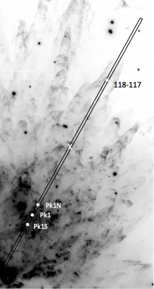
Figure 1: Image of a portion of the OMC-1 outflow in the H₂ 1–0 S(1) line (Bally et al., 2015) with the GNIRS slit superimposed. The midpoint of the 99-arcsecond long slit, indicated by the cross, is RA = 5:35:12.7, Dec = -5:21:41.25 (2000) and the position angle of the slit is -28.72^∘. The centers of the four segments of the slit from which spectra have been extracted are indicated by asterisks.

Whatever the explanation for the 5,000 K H₂ in HH 7, it is important to determine if similarly hot H₂ is common elsewhere in molecular gas that is excited by high velocity shocks. To begin to address this question, we have obtained $K$-band spectra of the brightest known region of line emission from shocked H₂, the energetic outflow in the Orion Molecular Cloud (OMC-1), in which the above mentioned dissociation speed limit is greatly exceeded (Nadeau & Geballe, 1979). Using the Frederick C. Gillett Gemini North telescope and its near-infrared spectrograph, GNIRS, with its long slit, we have simultaneously sampled a range of shocked gas environments in this cloud, from the region of brightest line intensity and broad line emission near Peak 1 (Beckwith et al., 1978) through one of the many Herbig-Haro objects in OMC-1 produced by high speed “bullets” (Allen & Burton, 1993).

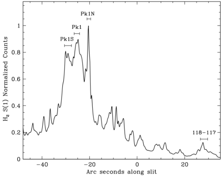
Figure 2: Intensity of H₂ 1–0 $S$(1) line emission along the GNIRS slit shown in Fig.1. The zero offset position corresponds to RA = 5:35:12.7, Dec = -5:21:41.25 (2000). Positive offsets are to the north-northwest. The regions from which spectra were extracted are indicated.

2 Observations and Data Reduction

Long-slit spectra covering 1.9–2.5 $\mu$m were obtained at Gemini North on UT 2015 November 6 and 8 for program GN-2015B-FT-3. The 0.45 $\times$ 99 arcsecond slit and the 32 lines/mm grating in GNIRS were employed, providing a resolution of 0.0018 $\mu$m, corresponding to a resolving power of $\sim$1200. This is considerably lower resolution than was used by PGBC to observe HH 7, and is insufficient to even partially resolve the H₂ velocity profiles in OMC-1 that have been observed by others. However, it is sufficient to separate the wavelengths of some of the critical (and very weak) high excitation H₂ lines from neighboring stronger H₂ lines, and from recombination lines from the foreground H II region.

Figure 1 is a portion of an image of the H₂  2.1218-$\mu$m 1–0 S(1) line emission, kindly supplied by J. Bally, on which the location of the GNIRS slit, oriented 28.72 degrees west of north, is superimposed. Using an offset from the bright star $\theta^{1}$Ori C the approximate midpoint of the sit was positioned half way between OMC-1 Peak 1, the region of brightest H₂ line emission, and one of the brighter OMC-1 bullets, approximately 55 arcseconds to the north-northwest, referred to as M42 HH120–114 by Tedds et al. (1999) and Finger 6 by Bally et al. (2017). Observations were obtained in the standard ABBA mode with the B position 90 arc-seconds to the west, where H₂ line emission from shocked gas is much weaker. The total on-source plus off-source exposure time was 48 minutes on each night.

Data reduction followed standard procedures, utlilizing flat-fielding, ratioing by the spectrum of the telluric standard star HIP 22189 for removal of telluric absorption lines and flux calibration, and observing the spectrum of an argon arc lamp for wavelength calibration. All of these measurements were obtained near-simultaneously with the spectra of OMC-1. Figure 2 shows the strength of the 1–0 $S$(1) line along the slit. After examination of this plot, four regions of bright H₂ line emission, shown in Fig. 1 and described in Table 1, were selected for detailed study. The three brightest of these are associated with Peak 1; the fourth lies in HH120–114 / Finger 6, approximately 10 arcseconds south-southwest of the tip of the shock as vewed in the Fe II 1.64-$\mu$m image of Bally et al. (2015). Hereafter we refer to this location in the nomenclature of Doi et al. (2002) as 118-117. For each of these regions the reduced spectra from the two nights, which were consistent with one another to within the noise, were aligned in wavelength and averaged to produce final spectra. The wavelength calibration is accurate to 0.0003 $\mu$m.

Table 1: Locations of Extracted Spectra

Name	Center RA & Dec	Area	$A$(2.2$\mu$m)
	(2000)	arcsec2	mags
Pk 1 S	5:35:13.63  -5:21:06.7	0.45 $\times$  3.00	1.14
Pk 1	5:35:13.52  -5:22:03.5	0.45 $\times$  2.25	1.10
Pk 1 N	5:35:13.35  -5:21:51.1	0.45 $\times$  1.50	1.39
118–117	5:35:11.80  -5:21:16.7	0.45 $\times$  3.30	0.22

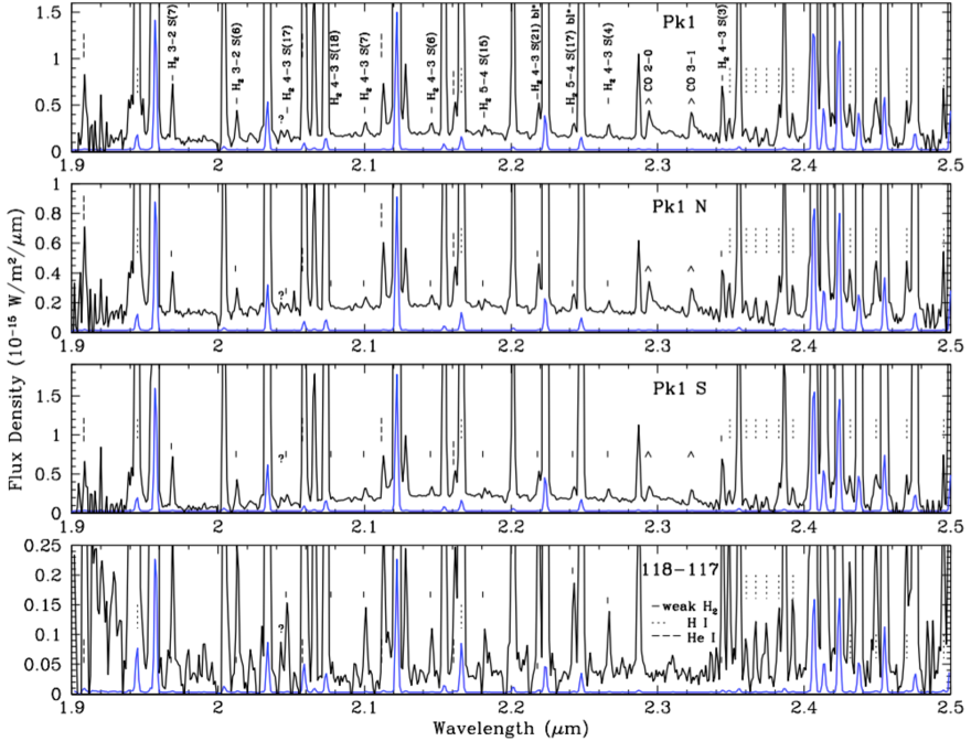
Figure 3: $K$-band continuum-subtracted spectra of four regions in OMC-1. H₂ 1–0 2.1218 $\mu$m $S$(1) line peaks are full scale in blue spectra. Spectra in black are magnified 100 times; the flux density scale applies to them. Strong H₂ lines are unlabeled; weak H₂ lines are indicated by tick marks and labeled at top. Lines of other species are indicated according to the legend at bottom. Blends of weak H₂ lines with [Fe III] lines are indicated by asterisks.

Table 2: Detected Lines

Rest $\lambda$	Species	Transition	Upper Level	Pk1 Flux	Pk1N Flux	Pk1S Flux	118–117 Flux	Notes
vac. $\mu$m			Energy (K)	10-18W m-2	10-18W m-2	10-18W m-2	10-18W m-2
1.9095	He I	4-3		yes	yes	yes	yes	yes = detected
1.9447	H I	8–4		yes	yes	yes	yes
1.9576	H2	1-0 $S$(3)	8,365	301	190	344	51.0
1.9692	H2	3-2 $S$(7)	23,070	1.10	0.54	1.16	0.42
2.0041	H2	2-1 $S$(4)	14,764	7.5	3.66	7.38	2.3
2.0130	H2	3-2 $S$(6)	21,912	0.73	0.35	0.74	0.53
2.0334	H2	1-0 $S$(2)	7,585	110	63.3	126	17.5
2.0430	uid			0.14	0.08	0.17	0.04
2.0475	H2	4-3 $S$(17)	42,022	0.15	0.08	0.23	0.32
2.0587	He I	$2^{1}$P - $2^{1}$S		yes	yes	yes	yes
2.0656	H2	3-2 $S$(5)	20,857	3.60	1.83	3.62	1.40
2.0735	H2	2-1 $S$(3)	13,890	27.6	15.5	29.6	6.90
2.0781	H2	4-3 $S$(18)	43,614	0.06	0.04	0.07	0.04
2.1004	H2	4-3 $S$(7)	27,202	0.40	0.22	0.43	0.27
2.1126	He I	4-3		yes	yes	yes	yes
2.1218	H2	1-0 $S$(1)	6,952	315	188	374	46.2
2.1281	H2	3-2 $S$(4)	19,912	1.76	0.90	1.75	0.51
2.1460	H2	4-3 $S$(6)	26,615	0.27	0.17	0.25	0.23
2.1542	H2	2-1 $S$(2)	13,151	12.1	6.21	11.7	2.75
2.1615	He I	7-4		yes	yes	yes	yes
2.1661	H I	7-4		yes	yes	yes	yes
2.1818	H2	5-4 $S$(15)	42,379	0.16	0.08	0.17	0.15
2.2010	H2	4-3 $S$(5)	25,624	1.51	0.83	1.60	0.52	blend; see PGBC
2.2014	H2	3-2 $S$(3)	19,087	4.54	2.51	4.82	1.56	blend; see PGBC
2.2184	[Fe III]			0.33	0.28	0.33	0.41	blend; see text
2.2196	H2	4-3 $S$(21)	48,345	0.33	0.28	0.33	0.41	blend; see text
2.2235	H2	1-0 $S$(0)	6,472	80.6	49.0	96.7	10.6
2.2427	[Fe III]			0.11	0.09	0.11	0.14	blend; see text
2.2433	H2	5-4 $S$(17)	45,275	0.23	0.15	0.28	0.10	blend; see text
2.2477	H2	2-1 $S$(1)	12,551	29.9	17.8	32.9	6.83
2.2666	H2	4-3 $S$(4)	24,734	0.27	0.19	0.38	0.24
2.2870	H2	3-2 $S$(2)	18,387	1.88	1.01	2.03	0.70
2.2935	CO	2-0 bh		yes	yes	yes	no
2.3227	CO	3-1 bh		yes	yes	yes	no
2.3445	H2	4-3 $S$(3)	23,955	1.17	0.83	1.39	0.80
2.3488	H I	29-5		yes	yes	yes	yes
2.3555	H2	2-1 $S$(0)	12,095	7.1	4.8	7.45	1.50
2.3604	H I	27-5		yes	yes	yes	yes
2.3669	H I	26-5		yes	yes	yes	yes
2.3744	H I	25-5		yes	yes	yes	yes
2.3828	H I	24-5		yes	yes	yes	yes
2.3863	H2	3-2 $S$(1)	17,819	4.77	2.91	4.66	1.48
2.3922	H I	23-5		yes	yes	yes	yes
2.4066	H2	1-0 $Q$(1)	6,149	308	193	375	35.9
2.4133	H2	1-0 $Q$(2)	6,472	108	64.5	125	12.1
2.4237	H2	1-0 $Q$(3)	6,952	274	173	328	33.8
2.4311	H I	20-5		yes	yes	yes	yes
2.4375	H2	1-0 $Q$(4)	7,585	90.0	55.6	107	12.1
2.4487	H I	19-5		yes	yes	yes	yes
2.4547	H2	1-0 $Q$(5)	8,365	128	76.5	158	23.1
2.4669	H I	18-5		yes	yes	yes	yes
2.4755	H2	1-0 $Q$(6)	9,286	46.3	26.7	49.1	7.2

3 Results

3.1 Detected Lines

The final reduced spectra of the four regions are shown in Fig. 3. Note that the the solid angles that they cover are not identical; they vary by over a factor of two (see Table 1). In each spectrum the continuum, which was determined by fitting a spline through wavelengths devoid of line emission, is subtracted. The strongest H₂ lines are much weaker at 118–117 (bottom panel of Fig. 3) than at the other positions; hence the spectrum as displayed there appears noisier.

A list of detected lines, including fluxes measured for the lines of H₂ (by numerical integration) is given in Table 2. More than half of the detected lines are from H₂. Recombination lines of H I (Brackett $\gamma$ and high $n$ lines from the Pfund series) are also present, as are a few lines of He I. We also tentatively identified two forbidden lines of Fe III, present in spectra by Youngblood et al. (2016) of other HH objects in OMC-1, and which are blended with weak high excitation H₂ lines. The latter three sets of lines presumably arise in the Orion Nebula H II region and are only partially removed by subtraction of the line emission at the nearby sky position, which also lies within the nebula. In addition, near 2.3 $\mu$m CO 2–0 and 3–1 band head emission is observable at the three locations near OMC-1 Peak 1. This is likely to be scattered emission that originated in the hot and dense disk surrounding the Becklin-Neugebauer object (Scoville et al., 1979) and possibly in disks of other other embedded young stellar objects within OMC-1.

The relative intensities of the H₂ lines in the three spectra near Peak 1 are nearly identical. The relative intensities in spectrum of 118–117 are strikingly different in two ways. First and most notably, the weak H₂ lines that can only be seen in the highly magnified spectra, are several times stronger relative to the strong lines at 118-117 than at the Peak 1 positions. Their fluxes are in fact comparable to their fluxes in the Peak 1 spectra, unlike those of the strong lines. The weak lines all arise from highly excited energy levels, as can be seen in Table 2. This hints at the existence of a high temperature component at 118–117 and/or a larger fraction of high temperature H₂ at 118–117 than at the other three locations. Second, at 118–117 the bright 1–0 $Q$-branch lines at 2.40–2.48 $\mu$m are much weaker relative to the bright 1–0 $S$(1-3) lines in the short wavelength portion of the spectrum. This implies significantly lower extinction to the shocked H₂ in 118–117 than at Peak 1.

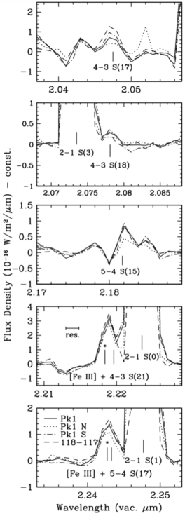
Figure 4: Spectra near the wavelengths of five weak, high excitation H₂ lines, shown for all four regions. Rest wavelengths of these lines and of nearby stronger H₂ lines are indicated by vertical lines. Forbidden lines of Fe III are indicated by vertical lines with asterisks.

3.2 The Highest Excitation Lines

As mentioned earlier, due both to the lower spectral resolution and to the presence of nearby line emission from other species, many of the H₂ lines from the highest energy levels that were seen by PGBC toward HH 7 were not detected at the four positions in OMC-1. Spectra in the vicinity of the five lines with upper energy levels exceeding 40,000 K that were detected are shown in Fig. 4 for all four regions. Three of the lines are well resolved from neighboring lines, but the 4–3 $S$(21) and 5–4 $S$(17) lines in the lower two panels are blended with forbidden Fe III lines; the latter line badly so. We estimate the fluxes in these H₂ lines as follows. The Fe III 2.2184-$\mu$m and H₂  2.2196-$\mu$m lines are shifted in wavelength from the center of the 2.219 $\mu$m emission feature by the same amount and thus probably contribute approximately equally to the feature. We thus have set the fluxes in the 4–3 $S$(21) line to half of the measured fluxes of the 2.219-$\mu$m feature. The spectra from Youngblood et al. (2016) indicate that the 2.2427-$\mu$m line of Fe III is about one-third the strength of the 2.2184-$\mu$m line of Fe III. We subtract these values from the 2.243-$\mu$m feature to derive the strengths of H₂ 5–4 $S$(17) line. The fluxes of the two H₂ lines, which are listed in Table 2, have higher uncertainties than the other weak lines. We have allowed for this by tripling their uncertainties. However, their effects on the model fits to the H₂ level populations are minor.

3.3 Fluorescent Contribution

Luhman et al. (1994) detected faint highly extended emission in the Orion Molecular Cloud from the 1–0 $S$(1) and 6–4 $Q$(1) lines of H₂, which they identify as ultraviolet induced fluorescence. This emission is superimposed on the emission from the collisionally shocked gas. The extent of the fluorescent line emission (at least 2 square degrees) is considerably greater than the of the line emission from shocked gas ($\sim$10 square arc-minutes). Luhman et al. (1994) estimate a fluorescent luminosity of 34  L_⊙ in the S(1) line alone. Averaged over the emission region the surface brightness of this fluorescent line is 150 times fainter than that of 118–117, the faintest region of shocked H₂ that we have examined. The small scale intensity distribution of the fluorescent emission is unknown, but the distribution is likely to be fairly smooth, unlike that of the line emission from the shocked gas. Thus subtraction of the fluorescent signal in the “sky” spectrum, obtained only 1$\farcm$5 distant is probably nearly complete. Moreover, the high excitation lines that most tightly constrain our analysis are emitted from rotation levels of 17 or higher. Radiative excitation of cold or even warm H₂ is unlikely to populate those levels. For all of these reasons we are confident that residual fluorescence makes a negligible contribution to the spectra of H₂ reported here and thus can be safely ignored in our analysis.

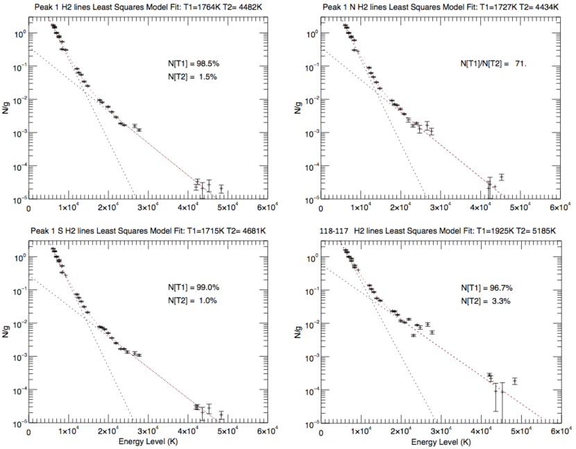
Figure 5: Level column densities, divided by their degeneracies plotted as a function of level energy for the shocked H₂ line emission. The y-axes are normalized to unity for the $(v,J)=(1,3)$ level (corresponding to the upper level of the 1–0 $S$(1) line). Error bars correspond to 1$\sigma$ values of 0.03 for the intensities listed in Table 2, for all but two weak lines for which they are 0.09 (see text). The curved dashed lines, the sums of the two straight dashed lines, are the best two-temperature LTE fits, for an ortho-to-para ratio of 3. Note the significant difference in the temperature of the hotter component at 118–117 compared to its values in the Peak 1 region, and the much larger percentage of hot gas at 118–117.

4 Analysis of the H₂ Spectrum and Results

Our method of analysis was the same as described in detail by PGBC. Briefly, after correcting the line fluxes for extinction (values given in Table 1), which was determined from the intensity ratios of the 1–0 $S$(1) and $Q$(3) lines, H₂ level column densities were calculated using decay rates from Wolniewicz et al. (1998) and line frequencies from Turner et al. (1977). The resultant population diagrams are shown in Fig. 5.

As in the case of HH 7, each of the four population diagrams is clearly indicative of gas at two distinct temperatures. The diagrams also demonstrate via the presence of significant populations in high rotational states that the higher temperature H₂ is not radiatively (UV) excited. We therefore modelled the population diagrams for two-temperature Boltzmann distributions as described in PGBC, again using the Levenberg–Marquard minimum-$\chi^{2}$ fitting routine and setting the maximum signal-to-noise ratio at 30 to avoid being constrained by the brightest lines, for which the uncertainties in flux are limited by systematic errors rather than random noise. The best fitting models are plotted in Fig. 5, along with the straight lines corresponding to the individual temperature components of which the model curves consist.

As was found for HH 7, at each location we examined in the OMC-1 shocked gas, a hot component of vibrationally excited H₂ is present at the few percent level and at a temperature similar to that of HH 7. At the Peak 1 locations the hot components have similar temperatures of 4,500 K to within the uncertainties (several hundred Kelvins), whereas the temperature of the hot component at 118–117 is $\sim$700 K higher and is essentially identical to the value found in HH 7. The temperature of the cooler bulk component at 118–117 is also higher than elsewhere in OMC-1, by roughly 200 K, and may be marginally higher than HH 7. Most interestingly, 118–117 also is significantly different from the Peak 1 positions and from HH 7 in that its percentage of hot H₂ is 2–3 times greater than at Peak 1 and is twice that of HH 7. Although the lines from the most highly excited levels (upper level energies in the range 40,000–50,000 K), whose strengths are most uncertain, are in part responsible for this conclusion, examination of the population diagrams (Fig. 5) shows that even in the range 20,000–30,000K the difference between 118–117 and the Peak 1 locations is obvious.

Goicoechea et al. (2015) have performed a similar anaysis of far-infrared (pure rotational) line emission from CO, H₂O and OH in the core of the Orion Molecular Cloud including the region near Peak 1. They too find multiple temperature components. The far-infrared line emission is dominated by molecular gas at much lower temperatures than that responsible for the H₂ vibration-rotation band line emission. However, at Peak 1 weak CO line emission is present from levels as high as $J$=48, 6,458 K above the ground state, comparable to the upper level energies of the strong 1–0 $S$(0) and $S$(1) lines of H₂. Their analysis indicates that this emission arises predominantly from gas at $\sim$2500 K. That gas likely also produces the bulk of the H₂ vibration-rotation band emission.

5 Discussion

The results of this paper, combined with the previous result of PGBC, strongly indicate that the presence of a small amount of $\sim$5,000 K H₂ is a common feature of molecular gas that is shocked by high velocity outflows and for which the temperature of most of the vibrationally excited H₂ does not exceed the typically observed value of $\sim$2,000 K. Despite the large scatter of the fluxes of the weak, high excitation lines in the population diagrams, it appears that the temperature difference between the high temperature H₂ (5,000–5,200 K) in HH 7 (PGBC) and 118-117 and the high temperature H₂ (4,400–4,700 K) at the Peak 1 locations is real.

PGBC tentatively concluded that the H₂ at $\sim$5,000 K has recently re-formed on grains after some of the H₂  either in the outflow or in the ambient gas, has been collisionally dissociated by the shock. However, as they discussed (see PGBC for details and references), how and why such gas should have a well-defined temperature is unclear. Some theoretical work on the energy level distribution of reformed H₂ that is just ejected from the dust grains on which it formed has indicated that is level distribution is unlikely to be thermal (Duley & Williams, 1986, 1993). More recent laboratory experiments, summarized in Williams et al. (2007), found that the internal energy of the H₂ after ejection from graphitic surfaces is less than 40% of the H₂ binding energy of 4.5 eV. As the observed temperature of $\sim$5,000 K, for the hot H₂ corresponds to 0.5 eV, the laboratory and astronomical results are consistent. The H₂ level populations in the laboratory experiment were not measured, however. Comparison of future such measurements with the astronomical data would be of great interest.

Even if the initial distribution of the reformed H₂ is thermal and at a temperature well above that of its surroundings, one might naively expect it to cool rapidly radiatively and/or collisionally and not to be characterized by a single well-defined temperature, but rather a range of temperatures. Modeling the time dependence of the energy level distribution starting from a variety of initial conditions and in a variety of environments could be illuminating, as would much more accurate astronomical measurements of the relative fluxes of some of the most highly excited lines.

Tedds et al. (1999) derived a shock speed of 120 km s^-1 near 118–117 by combining velocity profiles with proper motion measurements. Proper motion measuremements near Peak 1 are unavailable; however, examination of Fig. 5 of Bally et al. (2015) suggests that motions are relatively low there. The velocity profiles at Peak 1 (Nadeau & Geballe, 1979; Nadeau, Geballe, & Neugebauer, 1982), may then be indicative of actual wind speeds there. If so, they show that only a small fraction of the gas is moving at speeds approaching 120 km s^-1. Because higher velocity outflows impinging on ambient cloud material are more likely to lead to increased dissociation of H₂, qualitatively one would expect a higher percentage of the H₂ to be dissociated at 118–117 than at Peak 1 and likewise a higher percentage of re-formed H₂ there, as is apparently observed. However, it is unclear why the temperature of the reformed H₂ would be higher at those locations, as is apparently the case.

Finally, it would be of interest to observe the spectrum of H₂ at other locations in the OMC-1 outflow where speeds are considerably higher to determine if the fraction of high temperature H₂ is even greater than toward 118–117. Likewise, it would be of interest to observe the spectrum in lower velocity molecular shocks including in regions in which J-shocks, rather than C-shocks are thought to be the dominant interaction between outflow and cloud.

References

- Allen & Burton (1993) Allen, D. A. & Burton, M. G. 1993, Nature, 363, 54
- Bally et al. (2015) Bally, J., Ginsburg, A., Silvia, D., & Youngblood, A. 2015, A&A, 579, A130
- Bally et al. (2017) Bally, J., Ginsburg, A., et al. 2017, ApJ, submitted (arXiv:1701.01906)
- Beckwith et al. (1978) Beckwith, S., Persson, S. E., Neugebauer, G., & Becklin, E.E. 197, ApJ, 223, 464
- Brand et al. (1988) Brand, P. W. J. L., Moorhouse, A., Burton, M. G., et al. 1988, ApJ, 334, L103
- Chernoff et al. (1982) Chernoff, D. F., Hollenbach, D. J., & McKee, C. F. 1982, ApJ, 259, L97
- Doi et al. (2002) Doi, T., O’Dell, C. R., & Hartigan, P. 2002, ApJ, 124, 445
- Draine (1980) Draine, B. T. 1980, ApJ, 241, 1021 (Erratum 1981, ApJ, 246, 1045)
- Draine & Roberge (1982) Draine, B. T. & Roberge, W. 1982, ApJ, 259, L91
- Duley & Williams (1986) Duley, W. W., & Williams, D. A. 1986, MNRAS, 223, 177
- Duley & Williams (1993) Duley, W. W., & Williams, D. A. 1993, MNRAS, 260, 37
- Goicoechea et al. (2015) Goicoechea, J. R., Chavarría, L., Cernicharo, J., Neufeld, D. A., Vavrek, R., et al. 2015, ApJ, 799,102
- Hollenbach & Shull (1977) Hollenbach, D. J. & Shull, J. M. 1977, ApJ, 216, 419
- Kwan (1977) Kwan, J. 1977, ApJ, 216, 713
- London et al. (1977) London, R., McCray, R., & Chu, S-I. ApJ, 217, 442
- Luhman et al. (1994) Luhman, M. L., Jaffe, D. T., Keller, L. D., & Pak, S. 1994, ApJ, 436, 185
- Luhman & Rieke (1996) Luhman, K. L. & Rieke, G. H. 1996, ApJ, 461, 298
- Nadeau & Geballe (1979) Nadeau, D. & Geballe, T. R. 1979, ApJ, 230, L169
- Nadeau, Geballe, & Neugebauer (1982) Nadeau, D., Geballe, T. R., & Neugebauer, G. 1982, ApJ, 253, 154.
- Oliva & Moorwood (1988) Oliva, E. & Moorwood, A. F. M. 1988, A&A, 197, 261
- Pike et al. (2016) Pike, R. E., Geballe, T. R. Burton, M. G., & Chrysostomou, A. C. 2016, ApJ, 822, 82 (PGBC)
- Ramsay et al. (1993) Ramsay, S. K., Chrysostomou, A., Geballe, T. R., Brand, P. W. J. L., & Mountain, M. 1993, MNRAS, 293, 695
- Richter et al. (1995) Richter, M. J., Graham, J. R., & Wright, G. S. 1995, ApJ, 454, 277
- Scoville et al. (1979) Scoville, Hall, D. N. B., N. Z., Ridgway, , S. T., & Kleinmann, S. G. 1979, ApJ, 232, L121
- Tedds et al. (1999) Tedds, J. A., Brand, P. W. J. L., & Burton, M. G. 1999, MNRAS, 307, 337
- Turner et al. (1977) Turner, J., Kirby-Docken, K., & Dalgarno, A. 1977, ApJS, 35, 281
- Williams et al. (2007) Williams, D. A., Brown, W. A., Price, S. D., Rawlings, J. M. C., & Viti, S. 2007, Astron. Geophys., 48, 1.25
- Wolniewicz et al. (1998) Wolniewicz, L., Simbotin, I., & Dalgarno, A. 1998, ApJS, 115, 293
- Youngblood et al. (2016) Youngblood, A., Ginsburg, A., & Bally, J. 2016, AJ, 151, 173