New reconstruction of the sunspot group numbers since 1739 using direct calibration and ‘backbone’ methods

Abstract

Context. The group sunspot number (GSN) series constitute the longest instrumental astronomical database providing information on solar activity. This database is a compilation of observations by many individual observers, and their inter-calibration has usually been performed using linear rescaling. There are multiple published series that show different long-term trends for solar activity.

Aims. We aim at producing a GSN series, with a non-linear non-parametric calibration. The only underlying assumptions are that the differences between the various series are due to different acuity thresholds of the observers, and that the threshold of each observer remains constant throughout the observing period.

Methods. We used a daisy chain process with backbone (BB) observers and calibrated all overlapping observers to them. We performed the calibration of each individual observer with a probability distribution function (PDF) matrix constructed considering all daily values for the overlapping period with the BB. The calibration of the BBs was carried out in a similar manner. The final series was constructed by merging different BB series. We modelled the propagation of errors straightforwardly with Monte Carlo simulations. A potential bias due to the selection of BBs was investigated and the effect was shown to lie within the 1$\sigma$ interval of the produced series. The exact selection of the reference period was shown to have a rather small effect on our calibration as well.

Results. The final series extends back to 1739 and includes data from 314 observers. This series suggests moderate activity during the 18th and 19th century, which is significantly lower than the high level of solar activity predicted by other recent reconstructions applying linear regressions.

Conclusions. The new series provides a robust reconstruction, based on modern and non-parametric methods, of sunspot group numbers since 1739, and it confirms the existence of the modern grand maximum of solar activity in the second half of the 20th century.

1 Introduction

Observations of sunspots on the solar disc have been performed regularly since the advent of telescopes in the early 17th century. These measurements constitute the longest ongoing observational programme in astrophysics, providing important insights into solar activity and variability on centennial timescales.

However, these observations have been carried out by different people, with different instruments, at various locations. In some cases observations were taken for a different purpose but were also later used to define sunspot numbers. The definition of a sunspot group might have changed with time, gaps exist within the series of individual observers, and the various series do not necessarily all overlap with each other. Even for the same observer, the quality of the record may vary with time owing to, for example gaining experience, ageing of the observer (e.g. deteriorating eyesight), change of instrumentation, or varying conditions at the observing location. There have been several attempts to harmonize these measurements and to produce a homogeneous composite series. The first effort was made by Rudolf Wolf from Zürich who introduced the Wolf sunspot number (WSN) in 1848 (Wolf 1850, continued and updated as the international sunspot number, ISN), given by the formula

$$R_{s}=k(10\,G+S),$$ (1)

where $k$ is a weighting factor to normalize the various observers with each other, $S$ the number of sunspots, and $G$ the number of sunspot groups. It is important that, for the sake of homogeneity, data from only one primary observer were used for each day. If the data from the primary observer were not available for a given day, data from the secondary, tertiary, etc., observer were used, but only one observation was used per day, ignoring all other available data. The original records and notebooks of Wolf are not readily available now, implying that WSN cannot be re-constructed from scratch. This series contains annual values back to 1700, while monthly and daily values go back to 1749 and 1818, respectively. Since 1981 the WSN/ISN series has been synthesized by the Royal Observatory of Belgium (Clette et al. 2007), adapted to include all available observers for each day, rather than only the primary observer. The WSN/ISN series has been recently updated as version 2.0 by correcting for some proposed inhomogeneities (Clette et al. 2014).

More than a century after the work by Wolf, Hoyt & Schatten (1998) introduced the group sunspot number (GSN) series (HoSc98, hereafter), which is based on the number of sunspot groups only, neglects individual spots and includes data from all observers on the same day. The daily GSN is defined as

$$R_{g}=\frac{12.08}{N}\sum_{i}k_{i}G_{i},$$ (2)

where $k_{i}$ is the individual correction factor of the $i$-th observer, $G_{i}$ is the GSN reported by the $i$-th observer, $N$ is the total number of observers on the given day, and the constant 12.08 was introduced to match the average level of $R_{g}$ to that of $R_{s}$ over the period 1874–1976. The GSN series was designed to be more robust than WSN/ISN since it only considers sunspot groups and reduces uncertainties in the counts of individual sunspots. In addition, the GSN series includes a much greater number of raw data than WSN and is extended further back in time to 1610. An important advantage is that for the GSN series, a complete database of the raw data (published as Hoyt & Schatten 1998, and revised recently by Vaquero et al. 2016) is available, which makes it possible to reconstruct the entire series from scratch.

The homogenization and cross-calibration of the data recorded by earlier observers was always performed through a daisy-chaining sequence of linear scaling normalization of the various observers, using the $k-$factors. This means that starting with a reference observer, the $k-$factors are derived for overlapping observers. The latter data are in turn used as the reference for the next overlapping observers, etc. As is apparent, this leads to error accumulation in time when moving further away from the reference observer.

It has become obvious that the old series need to be revised because of the new-found data and the outdated methodology based on constant $k-$factors. The issue with such methods is twofold. Firstly, such methods assume that counts by two observers are proportional to each other, which is generally not correct. Secondly, the $k-$ factors are assumed to be constant for the entire operational period of each observer, whereas in reality the acuity of the observers and sensitivity of the instruments may vary with time. A dedicated activity of the research community (Clette et al. 2014) has led to several new sunspot series discussed below.

Cliver & Ling (2016, ClLi16, hereafter) have attempted to revise the GSN series using essentially the same methodology as Hoyt & Schatten (1998). They claim, however, that the earlier part of the Royal Greenwich Observatory (RGO hereafter) data (i.e. 41 years before 1915) might suffer from uneven quality owing to the purported learning curve process. Therefore, they corrected the GSN values over this period by normalizing them to the data by Wolfer using a second degree polynomial fit. The inhomogeneity of the early RGO data is still a matter of debate, however. Other studies did not find any extensive problem with RGO data: Sarychev & Roshchina (2009), Clette et al. (2014), and Lockwood et al. (2016b) reported as potentially problematic periods before 1880, 1900, and 1877, respectively, while data from Aparicio et al. (2014) and Carrasco et al. (2013) do not exhibit any apparent trend with respect to RGO data after $\sim$1885 and 1890, respectively. Thus, the period of 1874–1915 used by ClLi16 to ‘recalibrate’ the RGO dataset is not well defined. The ClLi16 series covers the period 1841–1980 and yields the highest level of sunspot activity in the mid-19th century among all available reconstructions.

Svalgaard & Schatten (2016, SvSc16, hereafter) also used the method of daisy-chaining $k-$factors. But these authors introduced five key observers (called ‘backbones’, BB hereafter) to calibrate each overlapping secondary observer to these BBs. Thus, they seemingly reduced the number of daisy-chain steps because some daisy-chain links are moved into the BB compilation rather than being eliminated. The problem with this method is that most of the BB observers did not overlap with each other. Thus their inter-calibration was performed via series extended using secondary observers with lower quality and poorer statistics. In the end, this introduces even more daisy-chain steps, since each BB observer is normalized to the neighbouring observer using a three-step procedure. The SvSc16 series also reduced the number of sunspot groups after 1940 by 7% to take into account the possible effect of the introduction of the Waldmeier classification of sunspot groups (Waldmeier 1939). However Lockwood et al. (2016a, c) have questioned the necessity for such a correction for the GSN. The SvSc16 series covers the period 1610–2015 and suggests a rather high level of solar activity in the 18th and, especially, 17th centuries.

All of these sunspot number series used calibration methods based on the linear scaling regression to derive constant $k-$factors. However, this linear $k-$factor method has been demonstrated to be unsuitable for such studies (Lockwood et al. 2016d; Usoskin et al. 2016a, b), leading to errors in the reconstructions that employ them.

An alternative method was proposed by Usoskin et al. (2016b, UEA16, hereafter), who calibrated each observer directly to the reference dataset, avoiding the daisy chain and error accumulation. The method is based on comparison of the active day fraction statistics of an observer with that in the reference dataset (RGO data for the period 1900–1976). The quality of each observer is characterized by the acuity observational threshold so that the observer is assumed to miss all sunspot groups that are smaller than this threshold, and to report all sunspot groups that are larger than this threshold. The acuity threshold for each observer is found by matching their active day fraction statistic with that of an artificially created reference dataset. The UEA16 series covers the period 1749–1995 and yields a moderate level of sunspot activity in the 18th and 19th centuries, lying between the HoSc98 and SvSc16 series.

Another revision of the GSN series was carried out by Lockwood et al. (2014) who corrected it for some apparent inhomogeneities. However, since this study is close to the HoSc98 series, we do not consider it separately here.

Thus, presently there are a number of sunspot reconstructions using different methods of calibration and yielding results that are inconsistent with each other. The most critical implication of these series is that they yield different long-term trends for the activity of the Sun (Lockwood et al. 2016b; Kopp et al. 2016). Over the 19th and 20th centuries, ClLi16 and SvSc16 show no trend, while HoSc98 and UEA16 show an increase in solar activity.

In an attempt to bridge the methodologies underlying previous studies and present more accurate error estimates, we present here a recalibration of the GSN data using an amendment of the most direct non-parametric calibration method described in Usoskin et al. (2016a). Similarly to SvSc16, we incorporate BB observers. However, the calibration of overlapping observers is performed with a non-linear non-parametric probability distribution function (PDF) derived from sunspot group counts for days when two observers overlap. This allows us to account for the error propagation in a straightforward manner. Calibration of the different resulting BB series is achieved with daisy chaining.

The data we use are introduced in Sec. 2. The procedure, including information about all individual BB observers and their processing is described in Sec. 3. Our composite series is presented and compared with other existing series in Sec. 4, where we also discuss the stability of our method and potential problems of our series. We summarize our results in Sec. 5.

2 Data

We employ the database of the sunspot group numbers recorded by individual observers that was recently published by Vaquero et al. (2016) as an update of the HoSc98 database. Observers are uniquely identified by their identification number in the database. Here we use these identification numbers as well.

We apply the following filters to these data:

• Data by Wolfer (1880–1928, id 338) were merged with those by Billwiller and Wolfer (1876–1879, id 335). The two series were combined together to a single series, since they do not directly overlap. The two series differ in that the former includes observations solely by Wolfer, while the latter includes observations made by both Wolfer and Billwiller. By merging these two series together, we can increase the length of the Wolfer series and its overlap with observations by Schmidt.

• Data from Flaugergues, H., Aubenas (1794–1795, id 22) were also merged with those from Flaugergues, H., Viviers (1788–1830, id 227) using the same procedure. These two datasets were obtained by the same observer, Flaugergues, who performed the bulk of his observations in Viviers, Ardéche, but who relocated to Aubenas for a period of about two years.

  The dataset from Aubenas contains merely 91 observations for these two years, a period of otherwise sparse observations (we have only nine records from all other observers used here). The overlap of the observations of Flaugergues from Aubenas to other observers is less than three days and does not provide adequate statistics to properly calibrate this series. Considering that the two locations are close to each other in the south of France, we make the assumption that the observing conditions were not significantly different. This enables us to merge the two Flaugergues series. Furthermore, because of the poor overlap with other series, inclusion of these data does not affect the rest of our series.

The HoSc98, ClLi16, SvSc16, and UEA16 series were downloaded from the SILSO (Royal Observatory of Belgium) website.

3 Calibration process

3.1 Algorithm and primary observers

We have developed an automated algorithm to perform the calibration of sunspot records by individual observers which includes the following steps:

• First, we selected primary BB observers who provided long and high-quality observations.

• Next, we calibrated the data from all other observers, denoted as secondary observers hereafter, to the primary BB observers using periods of overlapping observations (sufficient overlap is required, see Section 3.3), and produced the ‘BB series’, which are composites of data from the BB observer and all other observers calibrated to him/her.

• Individual BB series were cross-calibrated to each other, using the daisy-chain procedure.

• Finally, the composite series of daily GSN was constructed by averaging the calibrated BB series.

The calibration was carried out using a direct non-parametric method to a single reference dataset with a straightforward propagation of errors. No regression was used and the acuity of the observers was assumed constant over their entire observing life. The method is described in detail in Sec. 3.2

The selected sequence of the primary BB observers is Kanzelhöhe, RGO, Wolfer, Schmidt, Schwabe, Flaugergues, and Horrebow (see Table 1). The BB observers were selected to be those with sufficiently long observational records of high quality. We also used Schubert, Zucconi, and Hagen as stand-alone BBs. Because of the lacking bridge in the data in the middle of the 18th century, we were unable to directly calibrate these three observers to a single observer acting as a BB. Thus we did this by the extended statistics of the calibrated BB series. These observers are important since they cover periods over the 18th century when no other data are available. Our reference observer is RGO (but restricted to the period between 1900–1976) and all other BB series were calibrated to the level of RGO.

All data from RGO prior to 1900 were ignored when considering the primary BB observer because of the disputed inhomogeneity, as discussed in the Introduction. We discuss the effect of this decision on our calibration in Sect. 4.2.3.

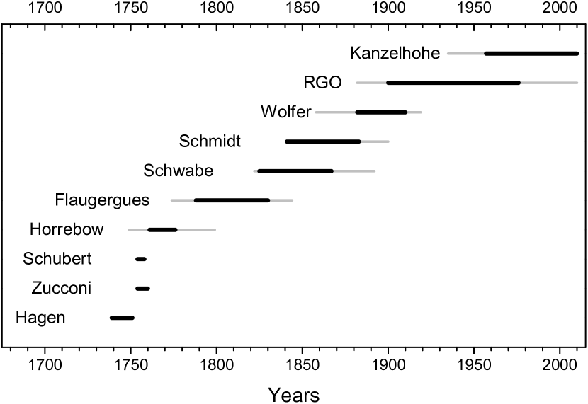
Figure 1: Temporal coverage by the BBs used here. Solid black lines represent the primary BB observers, while grey lines depict the extension of the BBs using calibrated secondary observers.

3.2 Secondary observers

Each BB series was also filled with all available secondary observers calibrated to the primary BB observers. As secondary observers we selected all the observers that have at least one nominal year of overlap with the primary BB observer. To avoid a distortion of statistics, each observer was included only in one BB. The assignment of observers to the BBs was made based on the length of the overlapping period and by trying to match observers with comparable quality BB observers. The only two successive BB observers whose observations do not overlap in time are Horrebow and Flaugergues. The bridging was made using Staudacher data. In this case, we chose Horrebow as the BB over Staudacher, because he observed more frequently and the data are of higher quality. Unfortunately, we were not able to go further back in time than Hagen (1739), because of the very sparse observations over this period with no observer making observations both before and after 1739 with adequate data to perform the calibration. Table 1 and Figure 1 provide key information about the BB observers and series.

All the observers we used for various BBs are listed in Tables 3 through 9. Figure 2 shows the number of days within each year covered by (a) the different BB series (i.e. including both primary and secondary observers) and by (b) our final composite series. One can see that the coverage is very good after ca 1800, but very poor in 1780–1795. This poorly covered period has led to large uncertainties in the daisy-chain method in the 18th century.

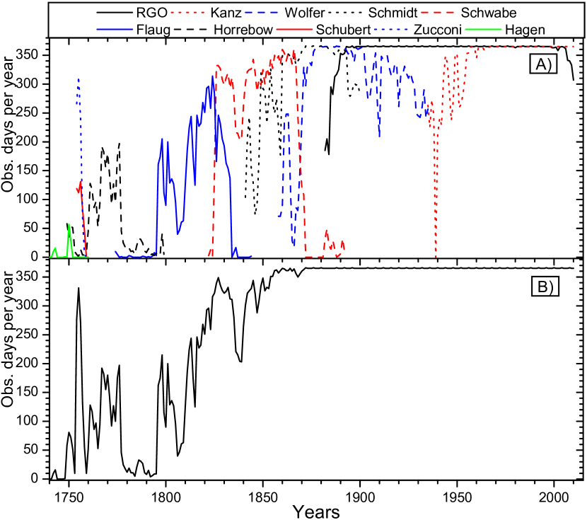
Figure 2: Annual coverage (number of observational days per year) by the different BB series (coloured curves in panel a) and by our final composite series (panel b).

Table 1: Backbones used in this study: name and identification (Id) of the primary BB observer; period covered by the BB composite series; period of observations of the primary observer; number of observers included in the BB series; number $N_{\rm d}$ of daily observations of the BB composite series; and direct daily overlap with the reference BB series, i.e. the number of days available in both BB series $M_{\rm d}$.

Backbone	Id	Period of observations		Observers	$N_{\rm d}$	$M_{\rm d}$
		series	primary observer
RGO	332	1882–2010	1900–1976	81	46087
Kanzelhöhe	606	1935–2010	1957–2010	156	25690	25526
Wolfer	335+338	1858–1919	1882–1910	25	22968	16601
Schmidt	292	1841–1900	1841–1883	11	18240	11708
Schwabe	279	1822–1892	1825–1867	22	14160	7386
Flaugergues	22+227	1774–1844	1788–1830	12	6948	1383 (1503)
Horrebow	180	1749–1799	1761–1776	4	2762	1775 (1795)
Schubert	178	1754–1758	1754–1758	1	492	10 (20)
Zucconi	177	1754–1760	1754–1760	1	899	17 (29)
Hagen	161	1739–1751	1739–1751	1	116	21 (34)

3.3 Construction of the backbone series

We started by building a direct calibration matrix (cf. Usoskin et al. 2016a) between the secondary observer to be calibrated and the primary BB observer for the days when both have observations. If, on a given day, $N_{1}$ and $N_{2}$ groups were recorded by the primary and secondary observers, respectively, then unity was added to the row $N_{1}$ and column $N_{2}$ of the matrix. In this way, the matrix was filled with all the overlapping days. Then the matrix was normalized such that each of its values were divided by the total sum over the corresponding column. Thus, we obtained a matrix of probability density functions (PDF) to find a value of $G^{*}$ reported by the primary observer for each day with the given value $G$ reported by the secondary observer. This allows a direct calibration of the secondary observer to the primary observer by replacing the $G$ value with the PDF of $G^{*}$. This is the most straightforward method for calibration applied directly to the data.

However, this matrix can potentially have some gaps due to poor statistics and limited range of overlap between the observers. In such cases, we fill the gaps by fitting the statistically significant part of the matrix with a function

$$\langle G^{*}\rangle-G=R_{0}+Be^{-aG}\,,$$ (3)

where $\langle G^{*}\rangle$ are the mean counts of the primary observer (i.e., the mean of the PDF of each column of the matrix) for a given count of the secondary observer $G$, $R_{0}$, $B$, and $a$ are constants calculated for each pair of observers individually. We used the weighted least mean squares to find the best-fit parameters. This functional shape (asymptotic exponential approach to a constant offset in the difference) was proposed by Usoskin et al. (2016a) and found suitable for this kind of dependence, using synthetic data that were based on RGO sunspot group area data.

Only those columns of the matrix that contain more that 20 overlapping days were included into the fitting procedure. If the fit deviated by more than one group from the actual mean $\langle G^{*}\rangle$, such columns were excluded, and the fit was redone. In such cases we refilled the column matrices using a PDF derived with a bootstrap Monte Carlo (MC, hereafter) simulation. For this, we randomly selected half of the overlapping days from the two observers, reconstructed the matrix using this half-statistics and recalculated the fit for the matrix. This process was repeated 1000 times. The result of this simulation was used as a PDF for the corresponding column in the matrix.

An example of the matrix is shown in Figure 3a for Winkler (secondary observer, $G$) and RGO (primary reference observer, $G^{*}$) over the period of their overlap (1900 – 1910 with 2480 common days). It is apparent that RGO typically reported more groups than Winkler for the same day, since most of the matrix values lie above the line expected for a perfect match between the two (black line). The matrix of the difference, $G^{*}-G$ versus $G$, is shown in Fig. 3b. The red circles with error bars represent the mean $\langle G^{*}\rangle$ value in each $G$ column and its (asymmetric) $1\sigma$ intervals. The green curve shows the best fit of the functional form of Eq. 3. It is obvious that the relation between $G^{*}$ and $G$ is non-linear and cannot be represented by a simple linear scaling $k-$factor. One can see that, because of the limited overlap, the matrix is well constructed only for $G<9$. For higher values, the fit (Eq. 3) has to be used. The full matrix with the values filled with the MC method for $G>8$ is shown in Fig. 3c.

Each secondary observer was calibrated to the BB observer by replacing, from the matrix, every daily count $G$ with the PDF of the calibrated counts $G^{*}$. In this way we directly convert the observations of the secondary observer to the BB condition without making any assumption about the type of relationship (e.g. linearity) and with a straightforward error estimate.

For each BB we constructed a composite series by averaging all the PDFs of all the available observations for every day, so that again, instead of one count for each day, we get a distribution based on all available observers. This composite of averaged PDFs includes possible errors in a straightforward way.

Only observers with a sufficiently long record of relatively good quality were included into the analysis. The selection of secondary observers was made using the following criteria:

1. The overlap with the primary BB observer should be not less than 20 common days of observations. This criterion was not applied for early years (see Section 3.3.1).

2. Observers with an overall record longer than 10 years were considered only if their overlap with the primary BB observer was at least 4 years. This is merely to make sure that long-running observers are not calibrated with a small fraction of their observations that might not be representative.

3. In cases in which we need to perform the fit to extrapolate to missing values in the matrix, we requested the conversion matrix for a selected observer to have sufficient data to cover at least three $G-$value bins. This is necessary since the function described by Eq. (3) has three parameters.

4. The matrix should cover, with sufficient statistics, at least one-quarter of the range of counts reported by the secondary observer.

5. Observers were excluded from the analysis if the difference matrix (see an example in Fig. 3b) had an average offset of more than two groups for the $G$ values from 0 to 5.

6. Observers, whose data could not be fitted accurately enough ($\chi^{2}$ per degree of freedom $<6$), were also excluded.

After the calibration process of all observers, we compared each individual observer with the composite BB series they were part of. We excluded those that showed significant and systematic discrepancies. Four observers were removed as they showed such differences, namely Taipei observatory (Id 456), Lunping (Id 457), Mojica, Cochabamba, Bolivia (Id 628), and XE (Id 715). We also excluded the Locarno station (Id 614), because of the possible lack of stability after 1980 (Clette et al. 2016).

\begin{overpic}[width=433.62pt]{winkler_a.eps} \put(17.0,34.0){a)} \end{overpic}

\begin{overpic}[width=433.62pt]{winkler_b.eps} \put(17.0,34.0){b)} \end{overpic}

\begin{overpic}[width=433.62pt]{winkler_c.eps} \put(17.0,34.0){c)} \end{overpic}

Figure 3: Example of the construction of the calibration matrix for Winkler (secondary observer, $G$) to RGO (primary, $G^{*}$) over 1900–1910. Panel (a) shows the original distribution matrix $G^{*}$ vs. $G$: the black line has a slope of unity. Panel (b) shows the difference, $G^{*}-G$ vs. $G$. Panel (c) is the same as (b) but the empty columns for $G^{*}>8$ have been filled with the results of the MC simulation. The red circles with error bars depict the mean $G^{*}$ values for each $G$ column and their 1$\sigma$ uncertainty. The yellow line shows the $k-$factor used in Hoyt & Schatten (1998).

There are also some special cases, which are described below in detail.

3.3.1 Sparse data: Schwabe and earlier backbones

Because of the lack of data for the first years of the Schwabe BB, we have not applied the criterion 1 from the list above to his data. Furthermore, while constructing the calibration matrix we considered observations not only during overlapping days but also within $\pm$1 day; if there was no direct overlap, we first checked one day earlier and then one day later, making sure that no more than one pair entered the matrix. Possible errors due to short-lived groups are negligible compared to the gain of the increased statistical sample (Willis et al. 2016; Usoskin et al. 2016b). These relieved constraints were also applied to the BBs covering earlier periods, when the statistics were poor.

3.3.2 Correcting for low quality observations: Flaugergues, Schubert, Zucconi, and Hagen backbones

For most BBs, we were able to match observers with a relatively similar quality. This was not the case for Flaugergues, though. Flaugergues’ data are very important, because they are the only record covering a relatively extended period in the early 1800s. However, the $G$ values he reported are significantly lower than those by other observers during that period, implying that his observations are of lower quality (higher acuity observational threshold). Therefore, a calibration of all other observers, with higher quality data, directly to Flaugergues would reduce their quality while increasing the uncertainties. In order to avoid that, we made use of a corrected Flaugergues series, calibrated to the mean level of the other observers of the period. In order to make the correction, we assumed that the acuity threshold for Flaugergues is $A=100$ msd, which is greater than for any other observer (Usoskin et al. 2016b). In this case the acuity threshold for Flaugergues does not even have to be the correct one, but it only should allow us to calibrate the overlapping observers without downgrading their quality. Applying the 100 msd threshold and the method described in Usoskin et al. (2016a), we obtained the following parameters for Eq. (3) for Flaugergues: $a=0.18$, $R=6.94$, and $B=6.03$. Then other observers were calibrated to this ‘corrected’ Flaugergues series.

The same process with the same threshold was used for the Schubert, Zucconi, and Hagen BBs.

3.4 Inter-calibration of backbone series

Once the BB series were constructed and calibrated to the primary BB observer, different BB series had to be inter-calibrated to each other. We used the RGO BB as the reference one, and the others were calibrated to it using a daisy chain. The calibration of the BB series was performed using a procedure similar to that for the individual observers, by constructing the cross-calibration matrix between the whole BB series this time. However in this case, we have, for each day, not a single $G$ value but a PDF from each observer (now the entire composite BB series is considered an observer). In order to account for that, we constructed the calibration matrix using a MC simulation as described below. For each day with simultaneous observations from both ‘observers’ (the BB series), we randomly selected $G$ values corresponding to the PDFs and filled the matrix. This process was performed 1000 times for each day, and the final matrix was computed as the average among all the individual matrices.

Monte Carlo simulations were used to calibrate the secondary BB to the reference one accounting for the error propagation. We randomly picked a $G$ value from the PDF for each day of the secondary BB series and obtained, from the matrix, the PDF of the $G^{*}$ values for the reference BB. This was repeated 1000 times and the average PDF of the $G^{*}$ values was considered as the calibrated PDF of the secondary BB series for that day.

The procedure is illustrated in Fig. 4, which shows the result of the calibration of the secondary Wolfer BB series to the primary RGO BB series. It is evident from the panel a) that the RGO BB $G$ values are systematically higher than those of the Wolfer BB (the difference is positive), implying that RGO is a better observer than Wolfer. After the calibration (panel b), the two series match each other so that the mean difference is consistent with zero in the entire range of $G$ values implying that the calibration was carried out correctly.

\begin{overpic}[width=433.62pt]{Wolfer_RGO_b.eps} \put(17.0,34.0){a)} \end{overpic}

\begin{overpic}[width=433.62pt]{Wolfer_RGO_d.eps} \put(17.0,34.0){b)} \end{overpic}

Figure 4: Difference between the Wolfer and RGO backbones. Panel (a) shows an uncalibrated matrix after the full MC filling; panel (b) shows the same matrix after the calibration. The red circles depict the average values in every column with their 1$\sigma$ uncertainty ranges.

This procedure works well for all the BBs. However, the results for the Horrebow BB series are very uncertain. The overlap of this series with the Flaugergues BB series is short and occurs only during activity minima around 1775 and 1795, which gives merely four points ($G$ values) to perform the fit and to extrapolate to the rest of the range of values. Since the method gives a realistic estimate of the uncertainties, this is clearly expressed in large error bars for the 18th century.

3.5 Construction of the final series

After all the BBs were calibrated to the reference RGO series, the final composite series was produced. First, for each day, all the available BB series values (in the form of a PDF) were merged into a single PDF for that day. From the daily PDFs of the calibrated $G$ values we produced the monthly $G$ values using a MC simulation. For this, for each day with available data within a month, we randomly selected a $G$ value from the final daily PDF and then computed the monthly value as the arithmetic mean of these daily values. This procedure was repeated 1000 times, and the PDF of the monthly values was constructed for each month. This MC method considers all the uncertainties straightforwardly. Finally, we collected the mean and asymmetric $\pm 1\sigma$ uncertainty level (a Table is available at the CDS).

Next, the annual numbers of sunspot groups with their asymmetric $\pm 1\sigma$ uncertainties were calculated from the monthly values in the same manner as monthly values from the daily values. The final annual series is given in Table 2 and shown in Figure 5. The GSN in years without reliable values are denoted by -99.

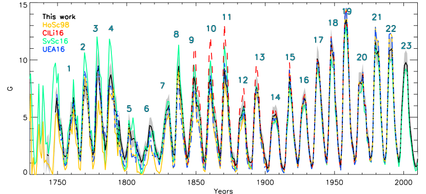
Figure 5: Annually averaged number of sunspot groups. This work is indicated in black with the $\pm 1\sigma$ area shaded; HoSc98 is indicated in yellow; UEA16 is shown in blue; SvSc16 is shown in green; and ClLi16 is indicated in red. Numbers on top of the curves denote the conventional solar cycle numbering.

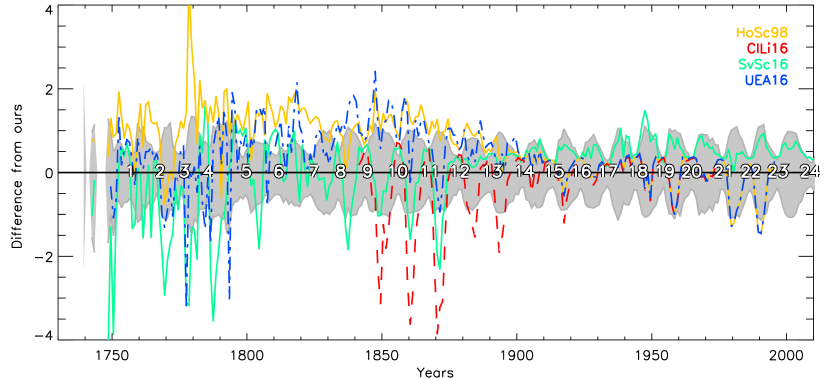
Figure 6: Differences of the annual GSN between our series and other series (as denoted in the legend). Positive values imply that our series is higher. The grey shading denotes the $\pm 1\sigma$ range of our series. The numbers denote the conventional solar cycle numbering.

Table 2: Annual values of the proposed GSN series with the asymmetric $1\sigma$ intervals.

Year	G	$\sigma_{+}$	$\sigma_{-}$	Year	G	$\sigma_{+}$	$\sigma_{-}$	Year	G	$\sigma_{+}$	$\sigma_{-}$	Year	G	$\sigma_{+}$	$\sigma_{-}$
1739	4.01	2.29	2.07	1799	1.74	0.52	0.49	1859	7.94	0.94	1.02	1919	6.00	0.77	0.79
1740	-99	-99	-99	1800	2.41	0.66	0.60	1860	8.34	0.95	0.99	1920	3.78	0.70	0.65
1741	-99	-99	-99	1801	4.42	0.93	0.84	1861	7.01	0.97	0.96	1921	2.65	0.65	0.58
1742	1.73	1.34	1.00	1802	3.69	0.88	0.72	1862	5.50	0.91	0.88	1922	1.59	0.51	0.40
1743	1.63	1.92	1.13	1803	3.01	0.75	0.70	1863	4.74	0.87	0.86	1923	0.92	0.38	0.32
1744	-99	-99	-99	1804	3.13	0.75	0.72	1864	4.47	0.88	0.85	1924	1.85	0.51	0.46
1745	-99	-99	-99	1805	3.13	0.71	0.68	1865	3.23	0.87	0.76	1925	4.22	0.76	0.70
1746	-99	-99	-99	1806	2.62	0.58	0.68	1866	2.27	0.71	0.58	1926	5.87	0.87	0.80
1747	-99	-99	-99	1807	2.09	0.47	0.67	1867	1.41	0.54	0.46	1927	6.28	0.76	0.80
1748	5.43	1.66	1.27	1808	1.86	0.65	0.43	1868	3.62	0.86	0.71	1928	6.72	0.88	0.92
1749	6.68	0.95	0.98	1809	1.52	0.54	0.44	1869	6.21	0.99	0.88	1929	6.05	0.80	0.73
1750	4.94	1.53	0.44	1810	1.08	0.49	0.42	1870	9.24	0.88	1.02	1930	3.83	0.77	0.64
1751	3.84	0.77	0.62	1811	1.27	0.55	0.42	1871	7.93	0.89	0.89	1931	2.39	0.53	0.48
1752	4.34	0.68	0.75	1812	1.92	0.51	0.61	1872	7.58	0.85	0.93	1932	1.31	0.42	0.34
1753	3.40	0.80	0.70	1813	2.26	0.70	0.49	1873	5.27	0.95	0.79	1933	0.72	0.35	0.27
1754	1.68	0.72	0.52	1814	2.04	0.62	0.51	1874	4.18	0.78	0.77	1934	1.05	0.40	0.32
1755	1.56	0.70	0.51	1815	3.22	0.76	0.64	1875	2.09	0.66	0.51	1935	3.75	0.75	0.64
1756	1.64	0.62	0.48	1816	4.26	0.75	0.78	1876	1.44	0.58	0.43	1936	7.45	0.91	0.80
1757	2.28	0.68	0.48	1817	4.20	0.80	0.76	1877	1.37	0.55	0.42	1937	10.10	1.15	1.03
1758	3.02	0.93	0.49	1818	3.78	0.80	0.75	1878	0.77	0.44	0.30	1938	9.72	0.96	1.06
1759	5.17	1.17	1.19	1819	3.04	0.76	0.62	1879	0.99	0.42	0.35	1939	8.10	0.76	0.76
1760	5.17	1.07	0.97	1820	2.42	0.63	0.53	1880	3.03	0.75	0.64	1940	6.31	0.72	0.76
1761	6.72	0.74	1.16	1821	1.87	0.58	0.50	1881	4.93	0.89	0.81	1941	4.55	0.74	0.67
1762	5.44	0.87	0.73	1822	1.56	0.60	0.42	1882	4.98	0.81	0.77	1942	2.86	0.63	0.50
1763	4.35	0.77	0.69	1823	1.28	0.55	0.36	1883	5.43	0.95	0.78	1943	1.63	0.43	0.35
1764	3.58	0.72	0.70	1824	1.60	0.64	0.39	1884	5.98	0.87	0.79	1944	1.27	0.43	0.33
1765	1.73	0.67	0.42	1825	2.54	0.72	0.60	1885	4.88	0.74	0.80	1945	3.55	0.69	0.61
1766	1.55	0.48	0.46	1826	3.67	0.93	0.77	1886	2.79	0.70	0.63	1946	8.07	0.94	0.86
1767	3.64	0.71	0.56	1827	4.71	0.96	0.85	1887	1.66	0.54	0.49	1947	11.62	1.10	1.17
1768	6.02	0.95	0.81	1828	5.54	0.97	0.95	1888	1.10	0.49	0.34	1948	10.59	0.98	1.00
1769	7.71	1.16	0.99	1829	5.71	0.95	0.94	1889	1.04	0.47	0.39	1949	10.04	1.01	0.91
1770	7.68	1.14	1.00	1830	6.03	0.99	0.99	1890	1.15	0.47	0.39	1950	6.47	0.88	0.86
1771	6.89	0.97	1.14	1831	4.34	0.94	0.85	1891	3.98	0.73	0.71	1951	5.19	0.79	0.76
1772	5.23	0.96	0.66	1832	3.08	0.81	0.69	1892	6.51	0.95	0.84	1952	2.74	0.55	0.55
1773	3.21	0.70	0.50	1833	1.77	0.61	0.53	1893	7.66	0.94	1.03	1953	1.46	0.48	0.42
1774	2.96	0.79	0.41	1834	1.70	0.71	0.50	1894	7.31	0.95	0.90	1954	0.74	0.32	0.27
1775	1.70	0.49	0.47	1835	4.69	0.91	0.82	1895	5.86	0.98	0.81	1955	3.33	0.65	0.55
1776	2.08	0.61	0.42	1836	8.32	1.08	0.95	1896	3.85	0.76	0.68	1956	10.29	1.03	1.05
1777	4.33	1.20	0.60	1837	9.47	0.83	1.17	1897	3.05	0.70	0.62	1957	13.03	1.01	0.97
1778	8.86	1.19	1.13	1838	7.29	1.00	1.05	1898	2.63	0.70	0.59	1958	13.50	1.05	1.10
1779	9.48	1.54	1.40	1839	6.49	1.03	0.93	1899	1.50	0.52	0.43	1959	11.71	0.91	0.93
1780	7.45	1.06	1.32	1840	5.12	1.01	0.86	1900	1.25	0.50	0.41	1960	8.53	1.05	0.96
1781	6.33	1.15	1.00	1841	3.40	0.77	0.77	1901	0.54	0.33	0.25	1961	4.45	0.75	0.75
1782	4.20	0.82	0.95	1842	2.42	0.79	0.60	1902	0.65	0.34	0.28	1962	2.91	0.57	0.57
1783	3.41	0.89	0.63	1843	1.35	0.62	0.42	1903	2.36	0.66	0.46	1963	2.35	0.53	0.45
1784	2.12	0.83	0.76	1844	1.78	0.68	0.54	1904	4.23	0.67	0.66	1964	1.20	0.42	0.30
1785	2.97	0.54	0.67	1845	3.61	0.86	0.80	1905	5.10	0.84	0.70	1965	1.58	0.46	0.38
1786	6.00	1.29	0.59	1846	4.57	0.94	0.85	1906	5.10	0.77	0.81	1966	3.97	0.68	0.66
1787	8.28	1.12	1.07	1847	6.82	0.92	1.18	1907	5.27	0.83	0.70	1967	7.88	0.98	0.90
1788	8.72	1.01	0.99	1848	8.55	0.87	0.97	1908	4.91	0.79	0.77	1968	8.03	0.93	0.90
1789	7.87	1.03	1.31	1849	7.89	1.06	0.90	1909	4.06	0.79	0.64	1969	7.90	0.98	0.89
1790	6.88	1.03	1.08	1850	5.96	0.93	0.91	1910	2.12	0.53	0.48	1970	8.75	0.89	0.85
1791	5.59	0.96	1.14	1851	5.99	0.98	0.96	1911	0.97	0.43	0.35	1971	6.07	0.77	0.81
1792	5.48	1.32	1.18	1852	5.48	1.03	0.96	1912	0.60	0.36	0.24	1972	5.94	0.88	0.85
1793	2.51	1.34	0.52	1853	4.33	0.87	0.82	1913	0.42	0.35	0.20	1973	3.40	0.66	0.68
1794	4.71	0.81	1.20	1854	2.55	0.82	0.66	1914	1.17	0.50	0.34	1974	3.12	0.68	0.63
1795	3.02	0.69	0.93	1855	1.33	0.49	0.47	1915	4.13	0.78	0.74	1975	1.57	0.43	0.41
1796	2.38	0.73	0.59	1856	1.10	0.60	0.38	1916	5.36	0.88	0.86	1976	1.41	0.39	0.35
1797	1.73	0.57	0.44	1857	2.95	0.76	0.70	1917	8.57	0.79	0.98	1977	2.65	0.57	0.53
1798	1.30	0.67	0.35	1858	5.44	1.05	0.87	1918	7.20	0.95	0.92	1978	7.92	1.04	0.80

4 Validation of the results

4.1 Comparison with other series

Other published GSN series are also shown in Fig. 5, but without the uncertainties. While all the series are dominated by the 11-year solar cycle, the centennial variability differs among different reconstructions. The ClLi16 and SvSc16 series are systematically higher than our reconstruction in the 19th and 18th centuries, while the HoSc98 series is somewhat lower. The present result is close to UEA16 and lies between the ‘high’ and ‘low’ models.

Figures 6 & 7 show the difference between various other series and the result presented here.

One can see that all the series agree with each other in the 20th century, except the SvSc16 series which is systematically lower than all others, although still within the error bars.

The UEA16 series is very close to our series during cycle maxima, while there are noticeable differences around the minima. The two series diverge for cycles 2 (our series is lower than UEA16), 8-9 (ours is higher), and 21-22 (ours is lower). The differences in cycles 22-23 can be explained by different observers used: while UEA16 used only RGO and Koyama over that period, we used here more than 150 observers, which allows us to estimate the activity more accurately.

During the solar cycle minima our series agrees with SvSc16, but there are distinct differences during the maxima. The SvSc16 series gives higher values over the cycles 1-5 and 8-11, while lower values are found for almost all cycles over the 20th century. These differences can be at least partly explained by the -7% ad hoc adjustment applied by SvSc16 to the data after 1940 and by the choice of Koyama as the reference observer (see also a discussion about this in Sec. 4.2).

Over the 20th century, the ClLi16 series is essentially the same as that of HoSc98, but they deviate over the 19th century so that maxima in the ClLi16 series are 3-4 groups higher than in HoSc98, and hence also than in ours. Keeping in mind that we ignored the RGO data before 1900 and used Wolfer as the reference for that period, the higher values by ClLi16 suggest a possible overcorrection of the RGO series by these authors. This is in agreement with the findings of Lockwood et al. (2016b).

In Figure 8 we show the secular trends of different series considered here, using the non-parametric SSA (singular spectrum analysis, Vautard et al. 1992). The SSA method is based on decomposition of a time series into several components with distinct temporal behaviours. It is very convenient for the identification of long-term trends and quasi-periodic oscillations, especially in the conditions when the secular trend is subdominant with respect to the main periodicity. As the secular trend we consider the first SSA components of the SN series. We used the time window for the SSA in the range of 80–100 years, where the result is stable. All series show that the activity level was highest in the late 20th century, corresponding to the modern grand maximum, but the relative enhancement differs among series. The greatest increase over the last 200 years (defined as the ratio of the values in 2000 and in 1750) is observed for the HoSc98 series ($\approx 2.6$), followed by the UEA (1.9) and our final series (1.7). Finally, SvSc16 series yields 1.3. Thus, the modern grand maximum is observed in all series. According to this work, this grand maximum is weaker than that in the HoSc16 series but greater than in the SvSc16 series.

4.2 Tests of stability

4.2.1 Choice of backbone observers

As primary BB observers, we selected those with sufficiently long observational periods of the best quality for each epoch. This is illustrated in Fig. 9, which shows the difference matrices for Wolf and Schmidt for two cases: Schmidt is considered as the primary observer and Wolf as the secondary (panel a) and vice versa (panel b). It is apparent that Schmidt was a better quality observer and is more appropriate to be chosen as the primary BB observer. By choosing Wolf as the BB observer, we would need to degrade Schmidt and other observers.

Table 2: (continued) Annual values of the proposed GSN series with the asymmetric $1\sigma$ intervals.

Year	G	$\sigma_{+}$	$\sigma_{-}$	Year	G	$\sigma_{+}$	$\sigma_{-}$
1979	11.61	1.06	1.02	1995	1.83	0.50	0.44
1980	10.50	1.00	1.04	1996	1.05	0.38	0.30
1981	10.78	1.05	1.08	1997	2.00	0.54	0.42
1982	8.85	0.99	0.88	1998	5.53	0.80	0.78
1983	5.52	0.89	0.79	1999	7.61	1.03	0.95
1984	3.56	0.70	0.59	2000	9.51	1.12	0.96
1985	1.51	0.50	0.38	2001	9.76	1.10	1.02
1986	1.19	0.43	0.31	2002	9.52	1.10	1.04
1987	2.28	0.50	0.51	2003	6.13	0.93	0.90
1988	6.65	0.93	0.84	2004	4.15	0.74	0.72
1989	10.81	1.01	1.00	2005	3.09	0.68	0.60
1990	10.86	1.16	1.11	2006	1.95	0.50	0.45
1991	11.00	0.98	1.11	2007	1.15	0.40	0.33
1992	7.46	1.04	0.84	2008	0.69	0.35	0.24
1993	4.53	0.72	0.63	2009	0.70	0.32	0.25
1994	2.96	0.64	0.56	2010	2.03	0.54	0.43

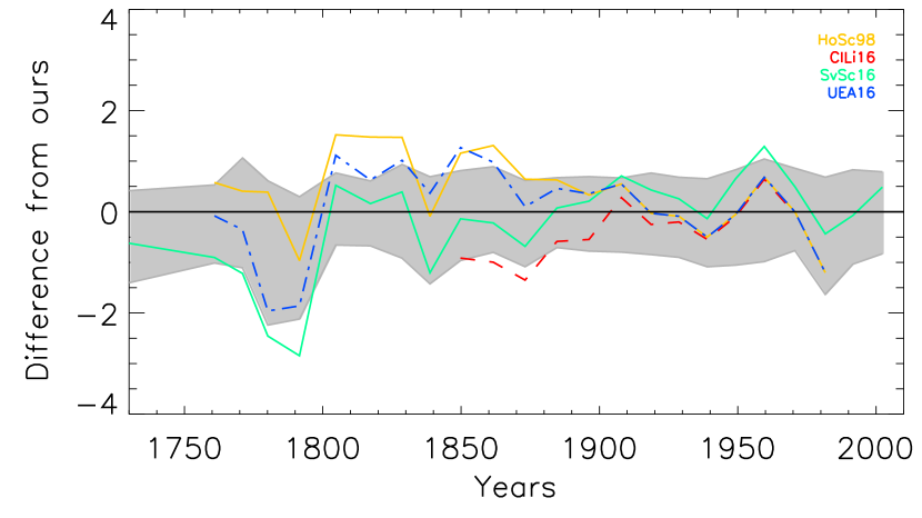
Figure 7: Differences of the solar cycle averaged GSN between our series and other series (as denoted in the legend). Positive values imply that our series is higher. The grey shading denotes the $\pm 1\sigma$ range of our series.

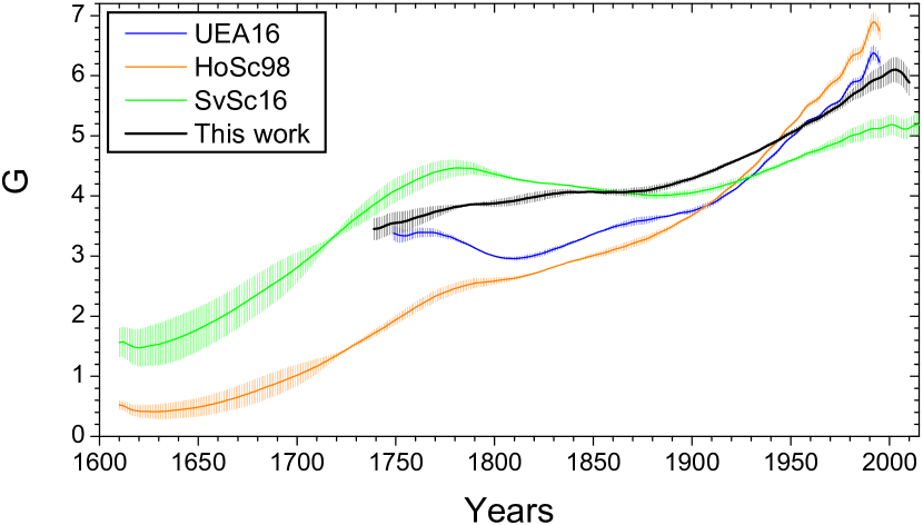
Figure 8: The long-term secular trend in different SN series, studied here, defined as the first SSA component. The shading represents only statistical uncertainties of the SSA method.

\begin{overpic}[width=433.62pt]{Wolf_Schmidt.eps} \put(17.0,34.0){a)} \end{overpic}

\begin{overpic}[width=433.62pt]{Schmidt_Wolf.eps} \put(17.0,34.0){b)} \end{overpic}

Figure 9: Matrices of the $G$ value difference between Wolf and Schmidt, where Schmidt (panel a) and Wolf (panel b) are selected as reference observers.

To test whether our final series is robust against the choice of the primary BB observers, we repeated the same analysis for different BB combinations. We used all possible combinations of high-quality long-lasting observers over four different intervals: (1) RGO (1900-1976), Koyama (1947-1984), Mt Wilson (1923-1958), (2) Wolfer (1880-1928), Quimby (1889-1921), (3) Schmidt (1841-1883), Spoerer (1861-1893), Weber (1859-1883), Wolf (1848-1893), (4) Schwabe (1826-1867), and Stark (1813-1836). This led to 48 alternative reconstruction series. Additionally, we constructed two more series by replacing Kanzelhöhe (1957-2010) with Cragg (1947-2009) and Locarno (1958-2010) and keeping all the other BBs as in the main series. Thus the total number of various GSN reconstructions was 50. We also included Flaugergues and Horrebow BBs in all series, but excluded the stand-alone BBs. The reference observer was chosen between RGO, Koyama, and Mt Wilson. Locarno has been excluded from all composites and our main series, however, we include it here as a BB to evaluate its effects on the calibration. We note that Quimby, as an individual observer, has overlap only with RGO, Wolf and Spoerer, while Stark has no overlap with any other BB observer used here. Thus, many of these auxiliary series result from disconnected BBs and are sometimes based on poor statistics. They can be used to assess uncertainties related to the BB selection, but as individual series, they are much less reliable than our main composite series. In this process, we did not exclude any other observers except those automatically rejected by the code (Sec. 3.3). The selection of observers within the BBs was performed automatically and may, of course, differ from those listed in Tables 3 - 9.

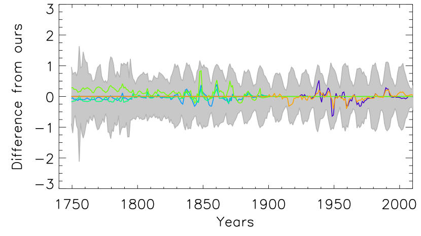
Figure 11: Difference between the main reconstructed series and the auxiliary series produced with different backbone combinations that include RGO, Wolfer, and Schwabe. Grey shaded area represents the $\pm 1\sigma$ uncertainties of the main series.

Figures 10 & 11 show the differences between our main series and the different auxiliary series, described above. The difference is mostly within the $\pm 1\sigma$ interval. Moreover, if the three main BB observers, i.e. RGO, Wolfer, and Schwabe, are fixed, the differences among the reconstructed series are quite small (Figure 11) and, thus, the choice of other BBs is not important. Using Koyama as the BB observer instead of RGO leads to systematically lower counts of sunspot groups (see blue curve in Figure 10), but these counts are still within the $1\sigma$ error bars.

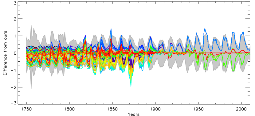
Figure 10: Difference between the main reconstructed series and all 50 auxiliary series produced with different backbone combinations. Annual values are shown. Grey shaded area indicates the $\pm 1\sigma$ uncertainties of the main series.

Thus, we can conclude that the method is stable regarding the exact choice of the BB observers with the potential uncertainty lying within the formal error bars.

4.2.2 Shape of the matrix

The majority of the calibration matrices constructed for individual observers have a shape (see Fig. 3) similar to that expected from synthetic data with an artificial acuity threshold applied (Usoskin et al. 2016a). This implies that the quality of an observer can be adequately quantified by his/her acuity observational threshold. However, distorted behaviour was found for some observers during periods of high solar activity, so that an observer, who is ‘poor’ (counting less groups than the reference observer) during periods of low and moderate activity, may appear to report more groups during solar activity maxima as if he/she were a better observer than the reference observer. This is caused by the low statistics and such columns in the matrix were replaced by the fit (Section 3.3). In the case in which this behaviour occurred over an extended region of the matrix, the observers were rejected by the code.

4.2.3 Quality of the RGO dataset

We also tested how crucial the choice of the exact reference period of the RGO dataset is. We repeated the same analysis, but considering the RGO dataset to start in 1874 and in 1916. Since a change of the reference period affects the statistics used for the calibration, allocation of some individual observers to specific BBs was automatically changed and was different than in Tables 3 through 9. Figure 12 shows the differences between the main series proposed here and these two alternative series. The result within the Kanzelhöhe BB is not affected at all, and for the rest of the BBs the difference is significantly smaller than the error bars, which are on average 0.14 and 0.10 for the annual values using RGO data for the periods of 1874–1976 and 1916–1976, respectively. At the same time, the use of the reference period shortened to after 1916 significantly decreases statistics, ignoring 42 years of RGO data. Thus, we conclude that the present reconstruction is also robust against the choice of the reference period of the RGO dataset.

4.2.4 Other issues

Our method may suffer from an intrinsic problem related to a possible overestimate of $G$ for periods of low activity. If a secondary ‘poor’ observer reports no spots, the method corrects it to a finite non-zero value of $G*$ (see e.g. Fig. 3). This is different from the linear $k-$factor method (e.g. SvSc16), in which zero values of a low-quality observer are always translated to zero values of the high-quality reference observer.

We explicitly assume, similar to all other SN reconstructions, that the observational record of any observer is error free in the sense that they report exactly the number of sunspot groups that should be visible to them on the Sun on a given day (cf. Spearman 1904; Wit et al. 2016). If this assumption were violated (e.g. weather or health conditions may temporarily reduce the acuity of the observer), the method would tend to slightly underestimate the reconstructed values at high activity levels, while overestimating the values at activity minima. However, at present there is no way to assess these kinds of errors and we have to rely on this assumption. We note that this also affects all other methods, including the linear k-factor.

We also assume (as is done in all other reconstructions) that the observational quality of an observer is constant in time. On the other hand, if it changed over time, especially outside the calibration period, it may introduce some additional uncertainties in the final result. However, in this work we cannot account for that and have to make the assumption on the constancy of the quality of the observer, as done by all the other reconstructions as well.

5 Summary and conclusions

We present a new reconstruction of the number of sunspot groups since 1739, along with realistic uncertainties, with daily, monthly, and annual time resolutions. The reconstruction is based on the daisy-chain normalization of individual observers via so-called ‘backbones’ built up on the records of the key observers of different epochs. In contrast to most of the previous works, based on a simple linear $k-$factor scaling (e.g. Hoyt & Schatten 1998; Clette et al. 2014; Svalgaard & Schatten 2016), our reconstruction employs a direct non-parametric calibration of observers by linking the values during days of simultaneous observations (Usoskin et al. 2016a). This method is based on the assumption that the quality of the data of the various observers is maintained throughout their observing period, which may not be well validated (Lockwood et al. 2016b). This will be studied elsewhere. We also assume, as all other methods do, that daily records of each observer are error free. A further assumption is that the main differences between the observers is due to their different observing capabilities. This assumption is used merely to extrapolate for the values that are missing from the overlapping period. Thus this method works with a minimum number of assumptions and allows for a direct comparison of two observers with different observational skills. Uncertainties of the reconstruction were assessed using a Monte Carlo method applied to the derived PDFs. This approach accounts naturally for the error propagation without making additional assumptions (e.g. about the normality and independence of errors). In other words, we present a highly advanced daisy-chain reconstruction of GSN based on the most direct calibration of observers.

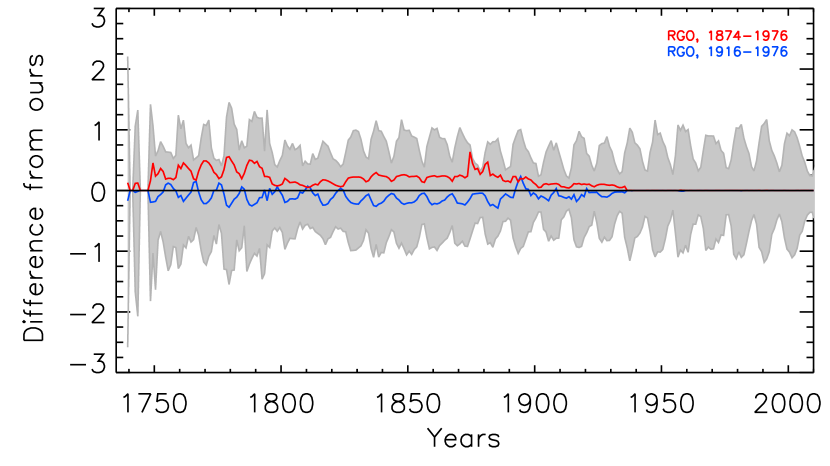
Figure 12: Differences between the main annual reconstructed $G$ series and those based on the reference RGO dataset for 1874–1976 and for 1916–1976 (blue and red, respectively). The grey shaded area depicts the $\pm 1\sigma$ uncertainties of the main series.

We tested the sensitivity of the method to the choice of the BB observers and of the reference period. We found that the reconstruction was robust and the result remained within the provided uncertainties.

The new series has been compared with other published GSN reconstructions, i.e. HoSc98, ClLi16, SvSc16, and UEA16. The new series lies close to UEA16, but is slightly higher than that in the 18th century. In contrast, it is systematically lower than ClLi16 in the 19th century and lower than SvSc16 in the 18th century. The latter two series are based on the $k-$factor scaling, which is shown to overestimate solar activity during solar cycle maxima (Lockwood et al. 2016d; Usoskin et al. 2016a, b). The new series confirms the existence of the modern grand maximum of activity in the second half of the 20th century, when sunspot cycles were significantly higher than during the 19th and 18th centuries.

The new GSN series provides a robust reconstruction of solar activity (the number of sunspot groups) with a realistic estimate of uncertainties and forms a basis for further investigation of centennial variability of solar activity over the last 270 years.

Appendix A List of observers

In this section we list all observers that were used in each BB series. The tables contain information on the Id of the observer in the Vaquero et al. (2016) database, the name of the observer, the first year of observations employed here, the last year of observations employed here, the number of daily observations $N_{\rm d}$ used, and the number of overlap days of observations with the BB observer $M_{\rm d}$ (for Schwabe, Flaugergues, and Horrebow BBs, the values for $\pm 1$ days are also given). The BB observer is listed first and the others are sorted based on their Id.

Table 3: List of observers used for the RGO backbone.

Id	Observer	Start	End	$\bf{N_{\rm d}}$	$\bf{M_{\rm d}}$
332	RGO	1900	1976	28124
341	Winkler, Jena	1882	1910	6161	2480
345	Konkoly, Ogyalla	1885	1905	3531	965
347	Stonyhurst College Obs.	1886	1935	4534	4338
352	Quimby, Philadelphia	1889	1921	10860	7428
358	Mount Holyoke College	1890	1925	2799	2774
361	Schwab, Kremsmunster	1892	1909	3619	2060
362	Catania	1893	1918	7620	5417
366	Sykora, Charkow	1894	1910	1883	1248
368	Lewitzky, Jurjew	1895	1907	1279	647
370	Broger, Zurich	1896	1935	9492	8600
376	Woinoff, Moscow	1898	1919	2881	2758
378	Freyberg, St. Petersburg	1898	1903	530	393
380	Kleiner, Zobten	1899	1918	1965	1823
381	Kitschigin, Spitzbergen	1900	1900	102	102
382	Subbotin, St. Petersburg	1900	1908	1017	1017
383	Gorjatschy, Moscow	1901	1908	603	603
384	Larionoff, Mohilew	1901	1903	202	202
385	Struve, Charkow	1901	1902	179	179
386	Guillaume, Lyon	1902	1925	6340	6340
387	Schatkow, Kola	1902	1910	1057	1057
388	Messerschmitt, Munchen	1902	1910	1715	1715
389	Stempell, Hannover	1903	1925	2760	2760
390	Amherst College Observatory	1903	1906	672	672
392	Morosoff, Moscow	1904	1909	58	58
394	Wasnetzoff, Moscow	1905	1912	455	455
395	Belar, Laibach	1906	1906	144	144
396	Hrase, Prague	1906	1916	1748	1748
397	Brunner, Chur	1906	1906	127	127
398	Bodocs, Ogyalla	1906	1916	1674	1674
399	Ginori, Florence	1907	1907	114	114
402	Sykora, Taschkent	1907	1907	155	155
403	Biske, Zurich	1908	1909	377	377
405	Lucchini, Florence	1908	1914	1190	1190
406	Guerrieri, Capodimonte	1908	1910	943	943
407	Braak, Batavia	1909	1925	1586	1586
408	Stefko, Leysin	1909	1913	260	260
409	Schwarz, Kremsmunster	1910	1914	654	654
411	Kavan, Prague	1911	1913	771	771
412	Moye, Montpellier	1911	1925	4744	4744
413	Miloradowitsch, Pulkowo	1913	1914	143	143
414	Buttlar, Simsdorf	1914	1925	1898	1898
417	Bugoslawsky, Moscow	1916	1918	411	411
419	Reed, Kennebunk, Maine	1917	1917	33	33
427	Mt. Wilson, Full Disk	1923	1958	11666	11666
428	Brunner, Zurich	1926	1944	4901	4901
429	Buser, Arosa	1928	1937	2722	2722
431	Brunner, W., Zurich	1929	1944	3262	3262
432	N.A.O., Japan, $k$=0.75	1930	1930	244	244
433	N.A.O., Japan, $k$=0.65	1931	1934	920	920
434	N.A.O., Japan, $k$=0.70	1935	1948	1293	1293
436	Waldmeier, Zurich	1936	1947	1615	1615

Table 3: List of observers used for the RGO backbone (continued)

Id	Observer	Start	End	$\bf{N_{\rm d}}$	$\bf{M_{\rm d}}$
437	N.A.O., Japan, $k$=0.55	1936	1936	207	207
438	Protitch, M., Belgrade	1936	1954	3357	3357
439	N.A.O., Japan, $k$=0.60	1937	1944	2059	2059
440	Rapp, Locarno-monti	1941	1944	1298	1298
441	Valencia Obs., Valencia	1920	1956	5734	5734
442	Waldmeier, Arosa	1942	1944	308	308
443	Djurkovic, P.M., Belgrade	1946	1946	159	159
444	Oskanjan, V., Belgrade	1947	1949	331	331
445	Koyama, H., Tokyo	1947	1996	9848	5746
446	U.S. Naval Observatory	1948	1956	3211	3211
447	National Astron. Obs., Japan	1949	1993	12243	7689
448	Simic, M., Belgrade	1949	1950	158	158
449	Dizer, M., Kandilli Obs.	1949	1954	691	691
451	San Miguel Obs., Argentina	1952	1965	1274	1274
452	Ozguc, A., Kandilli Obs.	1955	1968	1931	1931
454	Rome Observatory	1958	1989	7104	4758
458	Dogan, N., Ankara	1974	1975	455	455
464	Luft, H.	1924	1988	10628	7536
486	Athenes Eugenides, Greece	1967	1982	2386	1877
493	Athenes III, Elias, Greece	1949	1995	7611	4441
610	Luft 2, U.S.A.	1958	1988	4992	2662
612	Looks, Chile	1967	1987	3678	1906
655	Potsdam, Germany	1950	1999	5436	2740
658	Quezon, Philippines	1957	2010	10606	3709
667	Roma 3, Italy	1950	2000	4213	654
671	Santiago, Chile	1957	2005	3781	1356
679	Skalnate, Slovakia	1950	2010	9200	4379
681	San Miguel, Argentina	1967	2010	9400	2402
701	Uccle, Belgium	1949	2010	13283	5033
736	Cragg, T., Los Angeles	1947	2009	17726	8900

Table 4: Same as Table 3 but for the Kanzelhöhe backbone.

Id	Observer	Start	End	$\bf{N_{\rm d}}$	$\bf{M_{\rm d}}$
606	Kanzelhöhe Treffen, Austria	1957	2010	12862
435	Madrid Observatory, Madrid	1935	1986	11931	3453
453	Lee Observatory, Bierut	1956	1975	6532	3251
459	Space Environment Laboratory	1977	1995	6922	4764
460	Debrechen Heliophysical Obs.	1977	1977	365	268
461	Catania Observatory	1978	1987	3288	2055
462	Air Force Network	1981	1991	3572	2623
463	British Astron. Assoc.	1992	1995	1002	806
470	N.O.A.A., U.S.A.	1983	1994	2713	2071
472	Astr. Centre Ardenne, Belgium	1992	2003	1220	955
473	Andries Son, Belgium	2003	2010	1187	958
474	Antares, Italy	1994	1995	170	145
476	Aguilar, Valencia, Spain	1985	1988	967	729
477	Ahnert, Germany	1981	1988	1244	975
478	Andrew Johnston, Australia	2009	2010	221	168
479	Alcober Valencia Spain	1985	1990	1177	896
481	Ankara, Turkey	1977	1990	2898	2074
483	Philippe Wittelsheim, France	1989	2010	3984	3255
487	Australian Obs. Coonabarabran, Australia	1988	2007	5717	4325
488	G.O.A.S., Argentina	1987	1993	563	421
489	Observ. Paul Ahnert, Cottbus, Germany	1992	2010	4463	3431
490	Donostia, Spain	1991	1993	225	188
491	Athenes Nat. Obser. (1) 127, Greece	1981	1998	4247	3218
492	Athenes Nat. Obser. (2) 109, Greece	1981	1999	4391	3303
494	A4 Sanvito 32404, Italy	1986	2010	5971	4642
495	Balseiro, Uruguay	1983	1985	333	250
499	Obs.Jordano Dimitrovgrad, Bulgaria	1995	2005	1107	835
500	Bullon, Valencia, Spain	1982	2010	5225	4083
501	Bortolotti Mauro, Italia	1997	2009	3695	2989
502	Boscat Michael, Ca	2008	2010	466	397
504	Basrah, Iraq	1986	1986	228	168
505	Broxton Tony, U.K.	2008	2010	625	508
506	Bucharest, Romania	1981	1998	3828	2940
507	Bob Vanslooten, Netherlands	2009	2010	294	227
509	Beyazit Obser., Turkey	1981	1998	4532	3374
512	Courdurie Marcq En Baroeul, France	1989	2010	3516	2670
515	Claeys Vedrin, Belgium	1988	2010	5334	4169
518	Capricorno, Campinas, Brazil	1981	2009	3064	2233
521	Hans Coeckelberghs, Belgium	2006	2010	390	339
522	Fernandez Ruis, Santander, Spain	1992	2010	4059	3215
523	Culgoora Narrabri, Australia	1985	2010	4528	3484
524	De Backer Boom, Belgium	1983	2010	5485	4325
527	Deman, Belgium	1986	2010	568	471
529	Desrues, France	1981	1985	1289	933
530	Dubois Langemark, Belgium	1985	2010	6545	5071
533	Vasquez Carlos, Argentina	1991	2000	776	581
534	Ebro, Roquetes, Spain	1949	2010	16266	10698
536	Eleizalde, Caracas, Venezuela	1989	1999	3159	2411

Table 4: List of observers used for the Kanzelhöhe Backbone (continued)

Id	Observer	Start	End	$\bf{N_{\rm d}}$	$\bf{M_{\rm d}}$
436	Waldmeier, Zurich	1936	1947	1615	1615
548	Observatory Frantiska, Czech Republic	1997	2010	1657	1402
549	Stefaniks, Obs. Prague, Czech Republic	1997	2010	1551	1308
550	Fujimori Nagano, Japan	1968	2010	10558	7724
552	Gema Araujo, Spain	2000	2010	3105	2494
553	Andre Gabriel, Belgium	2006	2010	1497	1249
554	Grognard, Belgium	1981	1991	572	396
555	Gerard Dinant, Belgium	1981	2007	5031	3867
557	Gillissen, Belgium	1981	1993	2543	1925
558	German Morales, Cochabamba, Bolivia	1995	2010	4534	3530
560	Gollkowsky Rudolstadt, Germany	1982	1997	874	711
562	Schott Lutz, Gerd, Germany	2001	2010	2259	1839
563	Guillery Pulligny, France	1985	2005	2914	2395
565	Huancayo, Peru	1983	2006	1093	830
566	Hardie Jordanstown, N.Ireland	1989	1999	2427	1825
567	Hancharia, Italy	1995	1998	434	356
568	Helwan, Egypt	1967	2010	9743	6914
571	Mahmoud S, Mosque Society, Egypt	1995	2005	942	691
572	Holloman, U.S.a.	1983	2010	7498	5697
573	Hvezdaren Presov, Slovakia	1994	2010	3749	3013
576	Hazel Collett, United-kingdom	2003	2007	779	624
577	Hurbanovo, Slovakia	1969	2010	7859	6386
578	Hvezdaren Kysucke, Slovakia	1993	2010	4290	3414
581	Iskum, Budapest, Hungary	1989	1999	655	553
582	Iseo, Italy	1994	2005	1628	1389
583	Jambol, Bulgaria	1991	2003	698	532
584	Astro. De Reux Ciney, Belgium	1992	2010	3363	2647
585	Jef Claes, Belgium	2006	2010	799	654
586	Dragesco Jean, France	2002	2005	774	599
587	Jahn Jost, West-Germany	1987	1993	628	485
588	Observatory Haskovo, Bulgaria	1998	2001	240	186
589	Jorge Luis Garcia, Spain	1996	2010	1166	936
591	Johnston Gwynedd, England	1991	2009	3267	2486
592	Havana Solar Station, Cuba	2001	2010	2582	2057
595	Jeffrey Carels, Belgium	2006	2010	1027	874
596	Kawaguchi, Japan	1981	2010	8122	6151
597	Kandilli, Turkey	1950	2010	11250	7889
598	Karjali, Bulgaria	1992	1999	552	436
599	Kladno, Czech Republic	1993	2008	3507	2855
600	Koyama, Japan	1981	1996	3250	2401
601	Observatory Rokycany, Czech Republic	1997	2001	351	291
602	Kislovodsk, Russia	1981	2010	9069	6880
607	Larguier, France	1985	1994	2274	1754
613	Lieve Meeus, Belgium	2005	2010	909	766
615	Learmouth, Australia	1983	2010	7466	5614
616	Larissa Observatory, Greece	1989	2010	4751	3837
617	Lunping, Republic Of China	1981	1998	2965	2279
618	Manila, Philippines	1971	1988	5103	3562
620	Mac Kenzie, Dover, United-kingdom	1981	2010	8389	6421

Table 4: List of observers used for the Kanzelhöhe Backbone (continued)

Id	Observer	Start	End	$\bf{N_{\rm d}}$	$\bf{M_{\rm d}}$
621	Madrid, Spain	1978	1986	1036	734
622	Meadows Peter, U.K.	2008	2010	566	478
625	Michaux, Belgium	1986	1990	319	251
626	Murmansk, Russia	1994	2010	3041	2431
627	Milano, Italy	1994	2010	1805	1505
629	Roberto De Manzano, Italy	2003	2010	1984	1684
630	Mochizuki Urawa, Saitama, Japan	1978	2010	8007	5984
631	Mira Grimbergen, Belgium	1987	2010	2193	1719
632	Smolyan, Bulgaria	1990	2008	856	673
634	Juri Gagarin, Eilenburg, Germany	1992	2010	1818	1428
636	Obs. Copernicus, Varna, Bulgaria	1995	2002	494	352
639	Nijmegen, Netherlands	1983	2010	5344	4168
640	Barnes, Auckland, New-zealand	1985	2010	4037	3089
642	Obs. Solar Bernard Lyot, Brazil	1995	1996	178	121
645	O.M.A. Americana, Brasil	1987	1994	802	601
646	Ondrejov Observ., Czech-republic	1991	2010	4711	3890
645	O.M.A. Americana, Brasil	1987	1994	802	601
646	Ondrejov Observ., Czech-republic	1991	2010	4711	3890
649	Vlasim, Czech Republic	1989	1992	436	360
650	Palehua, Hawai	1983	1997	3512	2637
651	Perroni, Brazil	1981	1986	1413	1021
652	Pasternak, Berlin, Germany	1984	2010	5429	4331
654	Lormont, France	1991	1997	691	555
656	Observatory Prostejov, Czech Republic	1998	2010	1529	1273
657	Pyong Yang, Korea	1985	2003	4324	3306
659	Ramey, Puerto-rico	1983	2003	5957	4505
666	Rokycany - Luzicka, Czech Republic	1997	2001	424	348
668	Paulo Roberto Moser, Brazil	2010	2010	172	144
669	Rasson Mons, Belgium	1988	1997	2126	1626
670	Rodriguez, Venezuela	1986	1989	950	720
672	Siracusa II, Lapichino, Italia	1986	1995	365	294
673	Sjoerd Dufoer, Belgium	2007	2010	366	323
674	Sergio Fabiani, Bolivia	1995	1995	133	105
675	Sigma Octante, Cochabamba, Bolivia	1981	2010	5258	4049
677	Smith Marlyn, U.K.	2008	2010	379	313
678	San Jose, Buenos Aires, Argentina	1986	1996	702	531
683	Sobota, Slovakia	1992	2010	5258	4280
685	Saudi Arabia, Jeddah	1981	2010	5477	4154
688	Suzuki, Japan	1981	2010	7839	5954
691	Trento, Italy	1994	1994	48	48
692	Thomas Teague, United Kingdom	2005	2010	219	168
693	Central Weather Bureau, Republic Of China	1981	2010	5898	4564
694	Tangjungsari, Indonesia	1984	1989	1358	1031
696	Taipei 2, Republic Of China	1981	2005	3692	2796
697	Trieste, Italy	1967	1993	2704	2074
698	Spaninks Tilburg, Netherlands	1991	2010	3079	2424
700	Tony Tanti Naxxar, Malta	1986	1998	2271	1769
702	U.L.B., Belgium	1983	1986	594	463
705	Sliven, Bulgaria	1989	2003	1301	985
706	Ventura Mosta, Malta	1986	2003	3732	2834
709	Ruben Verboven, Belgium	2006	2010	154	135
713	Monte Mor, Brazil	2006	2010	729	625
717	Y Alarcos, Valencia, Spain	1986	1994	587	441
719	Yvergneaux Ronse-renaix, Belgium	1981	1997	3754	2844
720	Zagora, Bulgaria	1990	2010	2851	2307
721	Zamora, Spain	1993	1999	1138	865

Table 5: Same as Table 3 but for the Wolfer backbone.

Id	Observer	Start	End	$\bf{N_{\rm d}}$	$\bf{M_{\rm d}}$
335+338	Wolfer, Zurich	1876	1928	13533
329	Secchi, Rome	1871	1877	1530	298
333	Moncalieri	1874	1893	3598	2422
336	Aguilar, Madrid	1876	1882	1940	1381
337	Monthly Weather Review	1877	1886	2383	1786
339	Ricco, Palermo	1880	1892	3709	2668
343	Merino, Madrid	1883	1896	3221	2394
346	Vogel, Potsdam	1886	1886	162	135
347	Stonyhurst College Obs.	1886	1935	4534	1835
349	Schmoll, Paris	1888	1892	1359	1041
350	Haverford College Obs., PA	1888	1899	2063	1547
353	Carleton College Observatory	1889	1892	523	383
355	Smith Observatory	1890	1891	258	192
356	Hadden, D.E., Alta, Iowa	1890	1890	2964	2256
359	Schreiber, Kalocsa	1891	1895	1173	976
360	Zona, Palermo	1891	1891	282	233
369	Maier, Schaufling	1895	1901	632	529
373	Oliver, A.I., Boston U., MA	1897	1901	254	190
375	Jastremsky, B., Charkow	1898	1900	149	111
377	Mirkowitsch, Jaroslaw	1898	1900	135	111
379	Kaulbars, St. Petersburg	1898	1901	649	508
391	Boston University Obs.	1903	1906	359	239
401	Bemmelen, Batavia	1907	1919	2748	1910
415	Schmid, St. Gallen	1915	1915	225	173
421	Voss, Altona	1918	1918	198	145
465	Wolf, R., Zurich (small Telescope)	1858	1893	8285	4385

Table 6: Same as Table 3 but for the Schmidt backbone.

Id	Observer	Start	End	$\bf{N_{\rm d}}$	$\bf{M_{\rm d}}$
292	Schmidt, Athens	1841	1883	6970
298	Wolf, R., Zurich	1848	1893	18311	4153
307	Carrington, London	1853	1860	1215	204
311	Weber, Peckeloh	1859	1883	6983	4035
318	Spoerer, G., Anclam	1861	1893	6281	2449
323	Ferrari, Rome	1866	1879	478	429
324	Leppig, Leipzig	1867	1881	2611	1979
325	Dawson, W.M., Spiceland, Ind	1867	1890	1623	824
328	Tacchini, Rome	1871	1900	7584	2388
330	Billwiller, Zurich	1872	1875	308	286
331	Sawyer, E.F., Cambridgeport	1872	1874	282	273
342	Janesch, Laibach	1882	1887	1164	439

Table 7: Same as Table 3 but for the Schwabe backbone.

Id	Observer	Start	End	$\bf{N_{\rm d}}$	$\bf{M_{\rm d}}$	$\bf{M_{\rm d}}\pm$1day
279	Schwabe, H. Dessau	1825	1867	11945	11945
255	Stark, J.M., Augsburg	1826	1836	1075	924	1029
274	Herschel, J., London	1822	1837	122	37	61
278	Von Both, G., Breslau	1825	1826	183	59	72
280	Hussey, T.J., England	1826	1837	1207	879	1073
282	Lawson, H., Hereford	1831	1832	200	151	180
283	Ruprecht, H., Ziegenhain	1832	1832	39	31	35
284	Boguslawski, P.H.L., Breslau	1832	1832	17	14	17
285	Bohm, J.G., Wien	1833	1836	101	84	96
290	Petersen, A.C., Altona	1840	1841	13	10	13
294	Peters, C.H.F., Clinton, NY	1844	1870	1308	953	1028
299	Greisbach, T.J., England	1850	1865	168	161	168
300	Sestini, Georgetown	1850	1850	42	35	39
304	Pogson, N., London	1851	1851	13	11	13
305	Tomaschek, Wien	1852	1854	15	8	15
306	Borck, Cassel	1852	1855	19	19	19
308	Flagstaff Obs., Melbourne	1857	1858	16	15	16
312	Howlett, F., England	1859	1892	766	505	537
313	Baxendall, J., Manchester	1859	1859	7	7	7
314	Coast Survey, Washington	1860	1862	475	430	460
316	Jenzer, Bern	1861	1865	585	542	566
320	Waldner, Zurich	1863	1864	41	39	41
321	Meyer, Zurich	1864	1871	912	387	397

Table 8: Same as Table 3 but for the Flaugergues backbone.

Id	Observer	Start	End	$\bf{N_{\rm d}}$	$\bf{M_{\rm d}}$	$\bf{M_{\rm d}}\pm$1day
22+227	Flaugergues, H., Aubenas and Viviers	1788	1830	2101	2101
202	Bode, J.E., Berlin	1774	1822	68	26	32
218	Heinrich, P., Munich	1781	1820	396	119	216
236	Herschel, W., London	1794	1818	384	29	67
238	Gemeiner, A.T., Regensburg	1797	1797	3	1	3
245	Lindener, B.A., Glatz	1800	1827	519	114	210
246	Derfflinger, T., Kremsmunster	1802	1824	789	47	101
250	Prantner, S.M.J., Wilten	1804	1844	115	35	67
258	Tevel, C., Middelburg	1816	1836	858	89	156
260	Watts, Cape Diamond, Quebec	1816	1818	83	3	10
262	Adams, C.H., Edmonton	1819	1823	977	34	66
263	Pastorff, J.W., Drossen	1819	1833	1477	53	109
273	Arago, F.D., Paris	1822	1830	923	85	145

Table 9: Same as Table 3 but for the Horrebow backbone.

Id	Observer	Start	End	$\bf{N_{\rm d}}$	$\bf{M_{\rm d}}$	$\bf{M_{\rm d}}\pm$1day
180	Horrebow, C., Copenhagen	1761	1776	1532	1532
174	Lalande, J., Paris	1752	1798	105	15	26
185	Warschauer	1764	1766	3	2	3
203	Lievog, E., Copenhagen	1776	1777	196	97	101
466	Staudach, J.C., Nuremberg	1749	1799	1172	128	234