Thin-shell wormholes in 2+1-dimensional Einstein-Scalar Theory

Abstract

We present an infinite class of one-parameter scalar field extensions to the BTZ black hole in 2+1-dimensions. By virtue of the scalar charge the thin-shell wormhole supported by a linear fluid at the throat becomes stable against linear perturbations. More interestingly, we provide an example of thin-shell wormhole which is strictly stable in the sense that it is confined in between two classically intransmissible potential barriers.

I Introduction

Since the discovery of Bañados, Teitelboim and Zanelli (BTZ) black hole in $2+1-$dimensions, there has been a vast literature in the same context 1 ; 2 ; 3 ; 4 ; 5 ; 6 . Expectedly there has been a race to derive rival metrics to BTZ by employing new physical sources other than the cosmological constant 7 ; 8 ; 9 ; 10 ; 11 ; 12 ; 13 ; 14 ; 15 . As the problem amounts to introduce new physical sources it has become part of the classical field theory in curved spacetime. Just to mention a few, we note that they range from linear Maxwell 16 to non-linear electrodynamics 14 as well as scalar fields 8 ; 9 ; 10 , dilatons 7 ; 17 ; 18 ; 19 ; 20 ; 21 ; 22 ; 23 ; 24 ; 25 ; 26 , scalar multiplets 27 , Born-Infeld 28 , Brans-Dicke extensions 29 , etc.. In particular, recently we have obtained classes of scalar multiplet fields acting as sources of gravity in both $2+1$ and $3+1-$dimensions 27 . This method amounts to consider a set of scalar multiplets $\left\{\phi^{a}\right\}$ with the index ’$a$’ belonging to an internal gauge group, specifically the group $O\left(2\right)$ for $2+1$ and $O\left(3\right)$ for $3+1-$dimensions. However, upon deriving the field equations we had the freedom to reduce the problem to circular / spherical symmetry by suppressing the angular dependence and concentrating only on the modulus of $\left\{\phi^{a}\right\}$. The advantage in such a reduction ansatz is to pave the way towards technically solvable system of equations. The scope of the model can further be extended by adding a self-interacting potential. From physical considerations scalar multiplets are familiar field theoretical objects whose experimental construction may be feasible in a foreseeable future. The special case of a scalar multiplet is provided by a scalar singlet in which there is no internal gauge group . Our model considered herein is a massless scalar field singlet with an exponential potential of scalar coupled to gravity in $2+1-$dimensions 27 . Our system admits exact solutions with two parameters and can be considered yet another, one-parametric extension of the BTZ solution. After substitution of the solution for the scalar field the potential takes the form $V\left(r\right)=\frac{\text{const.}}{r^{\alpha^{2}}},$ where $\alpha$ is the crucial parameter in our model ranging over $0\leq\alpha<\infty,$ unless stated otherwise. Note also that the solution for $-\infty<\alpha<0$ can easily be mapped to the former case so that we make our choice of $\alpha$ in the range $0\leq\alpha<\infty.$ It can be anticipated easily that for $\alpha=0$ the resulting black hole solution reduces to the BTZ solution. We make use of the parameter $\alpha$, which can be phrased as ”scalar charge” together with the cosmological constant to establish a large class of Einstein-scalar solutions. Once this is accomplished the principal aim in the present paper is to employ this class of solutions to build thin-shell wormholes 30 ; 31 ; 32 ; 33 ; 34 ; 35 ; 36 ; 37 ; 38 ; 39 ; 40 ; 41 ; 42 ; 43 ; 44 ; 45 ; 46 ; 47 ; 48 ; 49 ; 50 ; 51 ; 52 ; 53 ; 54 ; 55 ; 56 . The role of the scalar field in such a construction is interesting: assuming a linear gas / fluid equation of state at the throat of the thin-shell wormhole allows us to make stable such wormholes. By stability it is meant throughout the paper, against small linear perturbations to preserve its identity through harmonic oscillations. Initial velocities at the throat of the perturbed fields may be considered in various ranges bounded only by the speed of light. These are called velocity dependent perturbations and they play important role in stability / instability checking analysis. When these are all taken into consideration we are able to show the existence of stability regions for our wormhole all by virtue of the role played by the scalar charge. Besides stability against linear perturbations we construct also thin-shell wormhole confined in between high potential barriers so that it remains forever stable in its potential well.

Organization of the paper is as follows. In Sec. II we present the Einstein-scalar field equations with the exponential potential and integrate them completely. Construction and dynamical analysis of the wormhole is investigated thoroughly in Sec. III. In Sec. IV we complete the paper with our concluding remarks.

II $2+1-$dimensional Einstein-scalar solutions

Before we start this section we comment that, recently a different approach has been employed by two of us to find similar results in Ref. 27 . The action in $2+1-$dimensional spherically symmetric, static theory of gravity coupled to a scalar field is given by ($8\pi G=1$)

$$S=\int d^{3}x\sqrt{-g}\left(R-\frac{1}{2}\partial_{\mu}\psi\partial^{\mu}\psi-\lambda e^{-\alpha\psi}\right)$$ (1)

in which $R$ is the Ricci scalar, $\psi=\psi\left(r\right)$ is the scalar field, $\alpha$ and $\lambda$ are coupling constants.

The line element is chosen to be

$$ds^{2}=-A\left(r\right)dt^{2}+\frac{dr^{2}}{B(r)}+r^{2}d\theta^{2}$$ (2)

in which $A\left(r\right)$ and $B\left(r\right)$ are unknown functions of radial coordinate $r$ to be found from the field equations. Explicitly the Lagrangian density becomes

$$\mathcal{L}=\sqrt{-g}R-\frac{r}{2}\sqrt{AB}\left(\psi^{\prime}\right)^{2}-\lambda r\sqrt{\frac{A}{B}}e^{-\alpha\psi}$$ (3)

where a prime denotes $\frac{d}{dr}$. The scalar field equation is obtained as

$$\psi^{\prime\prime}+\psi^{\prime}\left(\ln\left(r\sqrt{AB}\right)\right)^{\prime}+\frac{\lambda\alpha}{B}e^{-\alpha\psi}=0.$$ (4)

Einstein field equations can be derived directly by variation of the action in terms of $g^{\mu\nu}$ and they are given by

$$G_{\mu\nu}=T_{\mu\nu}$$ (5)

where $T_{\mu\nu}$ is the energy momentum tensor given by

$$T_{\mu\nu}=\frac{1}{2}\left(\partial_{\mu}\psi\partial_{\nu}\psi-\frac{1}{2}\partial_{\gamma}\psi\partial^{\gamma}\psi g_{\mu\nu}\right)-\frac{1}{2}\lambda e^{-\alpha\psi}g_{\mu\nu}.$$ (6)

Due to $\psi\left(r\right)$ which is a function of $r$ the explicit form of the energy momentum tensor components are calculated as

$$T_{tt}=\left(\frac{1}{2}\left(\psi^{\prime}\right)^{2}B+\lambda e^{-\alpha\psi}\right)\frac{A}{2},$$ (7)

$$T_{rr}=\frac{1}{2B}\left(\frac{1}{2}\left(\psi^{\prime}\right)^{2}B-\lambda e^{-\alpha\psi}\right)$$ (8)

and

$$T_{\theta\theta}=-\frac{r^{2}}{2}\left(\frac{1}{2}\left(\psi^{\prime}\right)^{2}B+\lambda e^{-\alpha\psi}\right).$$ (9)

Finally the explicit form of the Einstein’s equations are given by

$$\frac{B^{\prime}}{r}+\frac{1}{2}\left(\psi^{\prime}\right)^{2}B+\lambda e^{-\alpha\psi}=0,$$ (10)

$$\frac{BA^{\prime}}{r}-\frac{A}{B}\left(\frac{1}{2}\left(\psi^{\prime}\right)^{2}B-\lambda e^{-\alpha\psi}\right)=0$$ (11)

and

$$\frac{2ABA^{\prime\prime}-BA^{\prime 2}+A^{\prime}B^{\prime}A}{2}+\\ A^{2}\left(\frac{1}{2}\left(\psi^{\prime}\right)^{2}B+\lambda e^{-\alpha\psi}\right)=0$$ (12)

which together with (4) admit the following solutions

$$\psi\left(r\right)=\alpha\ln r$$ (13)

$$A\left(r\right)=\left\{\begin{array}[]{cc}C_{2}\left(r^{2}+\frac{\left(\alpha^{2}-4\right)C_{1}}{2\lambda}r^{\frac{\alpha^{2}}{2}}\right)&\alpha\neq 2\\ C_{2}r^{2}\left(C_{1}-\lambda\ln r\right)&\alpha=2\end{array}\right.$$ (14)

and

$$B\left(r\right)=\left\{\begin{array}[]{cc}\frac{2\lambda}{\alpha^{2}-4}r^{-\alpha^{2}}\left(r^{2}+\frac{\left(\alpha^{2}-4\right)C_{1}}{2\lambda}r^{\frac{\alpha^{2}}{2}}\right)&\alpha\neq 2\\ \frac{1}{r^{2}}\left(C_{1}-\lambda\ln r\right)&\alpha=2\end{array}\right.$$ (15)

in which $C_{1}$ and $C_{2}$ are two integration constants.

Let’s add that with $\alpha=0$ one finds $\psi=0$ and the action reduces to

$$S=\int d^{3}x\sqrt{-g}\left(R-\lambda\right)$$ (16)

in which $\lambda$ plays the role of a cosmological constant. The field equations admit the BTZ solution with 1 ; 2 ; 3

$$A=B=-M_{BTZ}-\frac{\lambda}{2}r^{2}.$$ (17)

Therefore for $\alpha\neq 2$ we set $C_{1}=-M_{BTZ}$ and $C_{2}=\frac{2\lambda}{\alpha^{2}-4}$ such that the $\alpha\rightarrow 0$ limit works correctly. Hence our metric functions for $0\leq\alpha<2$ can be written as

$$A\left(r\right)=\frac{2\lambda}{\alpha^{2}-4}\left(r^{2}-\frac{\left(\alpha^{2}-4\right)M_{BTZ}}{2\lambda}r^{\frac{\alpha^{2}}{2}}\right)$$ (18)

and

$$B\left(r\right)=\frac{2\lambda}{\alpha^{2}-4}r^{-\alpha^{2}}\left(r^{2}-\frac{\left(\alpha^{2}-4\right)M_{BTZ}}{2\lambda}r^{\frac{\alpha^{2}}{2}}\right)$$ (19)

with the potential

$$V\left(r\right)=-\frac{\lambda}{r^{\alpha^{2}}}.$$ (20)

For the case $\alpha=2,$ from (14) and (15) one can redefine the time and absorb the constant $C_{2}$ which means that we can set it to one.

Depending on the values of the free parameters, the general solution may admit black hole or naked singular spacetimes. But at any cost the solution is not asymptotically flat. Therefore to find the mass of the central object one can use the definition of Brown and York (BY) mass 57 ; 58 . Before we apply this formalism we would like to comment that other methods exist in literature which use the Noether’s theorem in order to find the conserved quantities including mass in a non-asymptotically flat spacetime. For $2+1-$dimensional BTZ solution we suggest to consult 59 ; 60 while for a wider study and comparison between these methods with the BY prescription one may look at 61 . Since our aim in the present study is to investigate Einstein Scalar thin-shell wormholes we delete the alternative analysis for the conserved quantities to a future study.

In accordance with the BY mass in a $D-$dimensional spherically symmetric spacetime with the line element

$$ds^{2}=-F\left(r\right)^{2}dt^{2}+\frac{dr^{2}}{G\left(r\right)^{2}}+r^{2}d\Omega_{D-2}^{2}$$ (21)

the BY mass is given by

$$M_{BY}=\\ \lim_{r_{b}\rightarrow\infty}\frac{D-2}{2}r_{b}^{D-3}F\left(r_{b}\right)\left(G_{ref}\left(r_{b}\right)-G\left(r_{b}\right)\right)$$ (22)

where $G_{ref}\left(r_{b}\right)$ is the reference function and $r_{b}$ stands for the radius of the boundary surface. Using (21) for the black hole solution with $0\leq\alpha<2$ we obtain $M_{BY}=\frac{M_{BTZ}}{4}$ and the line element can be written as

$$ds^{2}=-\frac{4}{4-\alpha^{2}}\left(\frac{r^{2}}{\ell^{2}}-\left(4-\alpha^{2}\right)M_{BY}r^{\frac{\alpha^{2}}{2}}\right)dt^{2}+\\ \frac{r^{\alpha^{2}}dr^{2}}{\frac{4}{4-\alpha^{2}}\left(\frac{r^{2}}{\ell^{2}}-\left(4-\alpha^{2}\right)M_{BY}r^{\frac{\alpha^{2}}{2}}\right)}+r^{2}d\theta^{2}.$$ (23)

in which $-\frac{\lambda}{2}=\frac{1}{\ell^{2}}.$ This solution includes the BTZ limit when $\alpha\rightarrow 0.$ This form of line element is valid only when $0\leq\alpha<2.$ For $\alpha>2$ the solution does not admit any known limit and therefore one has to consider the solution in its original form given by (14) and (15). In the rest of this work we impose $0\leq\alpha<2$ and the line element which we shall refer frequently is given by (23). Furthermore, $\alpha<0$ can be mapped to $\alpha>0$ and therefore we exclude it.

Before we finish this section we add that the field equations, in the limit of $\lambda\rightarrow 0$ admit

$$A\left(r\right)=\zeta r^{\frac{\alpha^{2}}{2}},$$ (24)

$$B\left(r\right)=\frac{1}{A\left(r\right)}$$ (25)

with $V\left(r\right)=0$ in which $\zeta$ is a new integration constant. Hence the line element becomes

$$ds^{2}=\zeta r^{\frac{\alpha^{2}}{2}}\left(-dt^{2}+dr^{2}\right)+r^{2}d\theta^{2}$$ (26)

which is the solution of Einstein-self interacting scalar field in $2+1-$dimensions.

III Thin-shell wormholes

Let’s consider the $2+1-$dimensional spherically symmetric static bulk spacetime, $\mathcal{M}$, given by (23) which can be written more appropriately as

$$ds^{2}=-\frac{4}{4-\alpha^{2}}\frac{r^{2}}{\ell^{2}}\left(1-\left(\frac{r_{+}}{r}\right)^{\frac{4-\alpha^{2}}{2}}\right)dt^{2}\\ +\frac{r^{\alpha^{2}}dr^{2}}{\frac{4}{4-\alpha^{2}}\frac{r^{2}}{\ell^{2}}\left(1-\left(\frac{r_{+}}{r}\right)^{\frac{4-\alpha^{2}}{2}}\right)}+r^{2}d\theta^{2}.$$ (27)

where $r_{+}$ is the radius of the horizon which is given by

$$r_{+}=\left(\ell^{2}\left(4-\alpha^{2}\right)M_{BY}\right)^{\frac{2}{4-\alpha^{2}}},$$ (28)

with $0\leq\alpha<2$. We consider a timelike hypersurface $\Sigma$ defined by

$$\digamma=r-a=0$$ (29)

in which $a>r_{+}.$ Next, we make two copies from the bulk located outside $\Sigma$, i.e., $r>a$ (let’s call them $\mathcal{M}^{\left(1,2\right)}$) and we paste them at the location of $\Sigma.$ The resulting manifold i.e., $\mathcal{M}^{\left(1\right)}\cup\mathcal{M}^{\left(2\right)}$ is a complete manifold with a throat located at the location of $\Sigma.$ For the smooth matching at the throat one has to apply the Israel junction conditions 62 ; 63 ; 64 which are given by, i) the induced metric tensor on either side of the throat must be identical i.e., $h_{ij}^{\left(1\right)}=h_{ij}^{\left(2\right)}$ and ii) the discontinuity of the extrinsic curvature must satisfy

$$k_{i}^{j}-k\delta_{i}^{j}=-8\pi GS_{i}^{j}$$ (30)

in which $k_{i}^{j}=K_{i}^{j\left(2\right)}-K_{i}^{j\left(1\right)}$, $k=$ $k_{i}^{i}$ and $S_{i}^{j}=diag\left(-\sigma,p\right)$ is the energy momentum tensor on the shell $\Sigma.$ Herein $K_{ij}^{\left(1,2\right)}$ is the extrinsic curvature tensor on the either sides of the throat defined by

$$K_{ij}^{\left(1,2\right)}=-n_{\gamma}^{\left(1,2\right)}\left(\frac{\partial^{2}x^{\gamma}}{\partial\xi^{i}\partial\xi^{j}}+\Gamma_{\alpha\beta}^{\gamma}\frac{\partial x^{\alpha}}{\partial\xi^{i}}\frac{\partial x^{\beta}}{\partial\xi^{j}}\right)$$ (31)

where $x^{\alpha}=\left\{t,r,\theta\right\}$ and $\xi^{i}=\left\{\tau,\theta\right\}$ are the coordinate systems on the bulk and the throat, respectively. The first condition is satisfied by setting

$$h_{ij}^{\left(1\right)}=h_{ij}^{\left(2\right)}=h_{ij}=diag\left(-1,a\left(\tau\right)^{2}\right)$$ (32)

such that the line element on the shell is given by

$$ds_{\Sigma}^{2}=-d\tau^{2}+a\left(\tau\right)^{2}d\theta^{2}$$ (33)

in which $\tau$ is the proper time on the shell. Let’s add also that in general the coordinates of either sides of the throat are related as $r^{\left(1\right)}=r^{\left(2\right)}=a\left(\tau\right)$, $\theta^{\left(1\right)}=\theta^{\left(2\right)}=\theta$ and

$$\left(\frac{dt^{\left(1,2\right)}}{d\tau}\right)^{2}=\left.\frac{1}{A^{\left(1,2\right)}}\left(\frac{1}{B^{\left(1,2\right)}}\left(\frac{da\left(\tau\right)}{d\tau}\right)^{2}+1\right)\right|_{\Sigma}$$ (34)

but due to the identical metric in either sides of the throat i.e., $A^{\left(1,2\right)}=A$ and $B^{\left(1,2\right)}=B$ they become equal i.e.,

$$\left(\frac{dt^{\left(1\right)}}{d\tau}\right)^{2}=\left(\frac{dt^{\left(2\right)}}{d\tau}\right)^{2}=\\ \left.\frac{1}{A}\left(\frac{1}{B}\left(\frac{da\left(\tau\right)}{d\tau}\right)^{2}+1\right)\right|_{\Sigma}$$ (35)

in which

$$A=\frac{4}{4-\alpha^{2}}\frac{r^{2}}{\ell^{2}}\left(1-\left(\frac{r_{+}}{r}\right)^{\frac{4-\alpha^{2}}{2}}\right)\text{ }$$ (36)

and

$$B=r^{-\alpha^{2}}A.$$ (37)

In (31) $n_{\gamma}^{\left(1,2\right)}$ are the normal vectors on both sides of the throat defined as

$$n_{\gamma}^{\left(1,2\right)}=\pm\left(\frac{\partial\digamma}{\partial x^{\alpha}}\frac{\partial\digamma}{\partial x^{\beta}}g^{\alpha\beta}\right)^{-\frac{1}{2}}\frac{\partial\digamma}{\partial x^{\gamma}}$$ (38)

in which based on (31) the $+$ and $-$ refer to $n_{\gamma}^{\left(2\right)}$ and $n_{\gamma}^{\left(1\right)},$ respectively, and explicitly they are given by

$$n_{\gamma}^{\left(1,2\right)}=\pm\left(-\sqrt{\frac{A}{B}}\dot{a},\frac{\sqrt{B+\dot{a}^{2}}}{B},0\right)_{\Sigma}.$$ (39)

Herein a dot implies the derivative with respect to the proper time $\tau.$ Following $n_{\gamma}^{\left(1,2\right)}$ we obtain

$$k_{\tau}^{\tau}=\frac{A^{\prime}\sqrt{B+\dot{a}^{2}}}{A}+\frac{2B\ddot{a}-B^{\prime}\dot{a}^{2}}{B\sqrt{B+\dot{a}^{2}}},$$ (40)

and

$$k_{\theta}^{\theta}=\frac{2\sqrt{B+\dot{a}^{2}}}{a}$$ (41)

which yield

$$\sigma=-\frac{\sqrt{B+\dot{a}^{2}}}{4\pi Ga}$$ (42)

and

$$p=\frac{A^{\prime}\sqrt{B+\dot{a}^{2}}}{8\pi GA}+\frac{2B\ddot{a}-B^{\prime}\dot{a}^{2}}{8\pi GB\sqrt{B+\dot{a}^{2}}}$$ (43)

in which a prime stands for the derivative with respect to $r$ and all expressions are at $r=a.$ Explicitly one can show that the energy conservation implies

$$\frac{d\left(\mathcal{A}\sigma\right)}{d\tau}+p\frac{d\mathcal{A}}{d\tau}=\Xi$$ (44)

in which $\mathcal{A}=2\pi a$ is the area of the throat and

$$\Xi=\frac{\left(BA^{\prime}-AB^{\prime}\right)\sqrt{B+\dot{a}^{2}}}{4GAB}\dot{a}.$$ (45)

If we assume that there exists an equilibrium radius $a=a_{0}$ where the throat of the wormhole is at rest with no acceleration, i.e., $\dot{a}=\ddot{a}=0,$ the energy density and lateral pressure become static. At such equilibrium condition one obtains

$$\sigma_{0}=-\frac{\sqrt{B_{0}}}{4\pi Ga_{0}}$$ (46)

and

$$p_{0}=\frac{A_{0}^{\prime}\sqrt{B_{0}}}{8\pi GA_{0}}$$ (47)

in which a sub$-0$ stands for the equilibrium state. Therefore if the radius of the throat is set to be $a=a_{0}$ we may consider the wormhole to be at equilibrium but it may not be a stable state. Therefore we perturb the throat which means we apply a force and change the radius of the throat. If after the perturbation the throat tends to go back to its initial equilibrium point we shall define the wormhole to be stable, otherwise unstable. To see if the throat goes back to its equilibrium point or not, one has to write an equation of motion for the throat. This equation is extracted from the dynamic expression of $\sigma$ given by Eq. (42). Hence, by rearranging the terms in (42) we find a one-dimensional classical motion of the form

$$\dot{a}^{2}+V\left(a\right)=0$$ (48)

where

$$V\left(a\right)=B-\left(4\pi Ga\sigma\right)^{2}.$$ (49)

To go further one has to identify $\sigma$ as a function of $a.$ This can be achieved by considering an equation of state (EoS) for the fluid presented on the shell. Here in this study we consider a linear EoS of the form

$$p-p_{0}=w\left(\sigma-\sigma_{0}\right)$$ (50)

in which $w$ is a constant. EoS (50) and the energy conservation (44) can be combined to find an explicit expression for $\sigma$. Our analytic calculation yields

$$\sigma=\frac{\left(2+\alpha^{2}\right)\sigma_{0}+2p_{0}}{2w+2+\alpha^{2}}\left(\frac{a_{0}}{a}\right)^{w+1+\frac{\alpha^{2}}{2}}\\ +\frac{2w\sigma_{0}-2p_{0}}{2w+2+\alpha^{2}}.$$ (51)

Upon (51), the potential function becomes

$$V\left(a\right)=B-\left(4\pi Ga\right)^{2}\times\\ \left(\frac{\left(2+\alpha^{2}\right)\sigma_{0}+2p_{0}}{2w+2+\alpha^{2}}\left(\frac{a_{0}}{a}\right)^{w+1+\frac{\alpha^{2}}{2}}+\frac{2w\sigma_{0}-2p_{0}}{2w+2+\alpha^{2}}\right)^{2}.$$ (52)

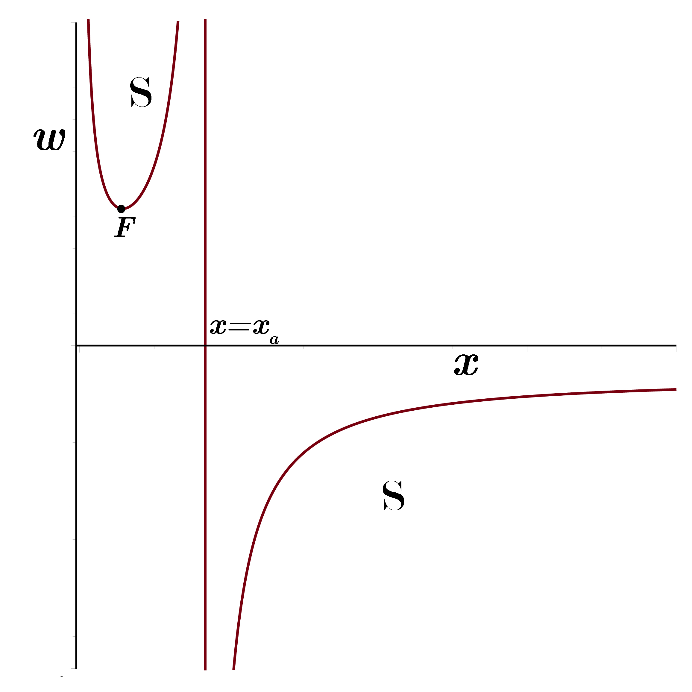
Figure 1: The general behaviour of $V_{0}^{\prime\prime}$ versus $x=\frac{a_{0}}{r_{+}}$ and $w$ for an orbitrary $\alpha^{2}<4.$ The parts labeled with $S$ shows the stable regions.

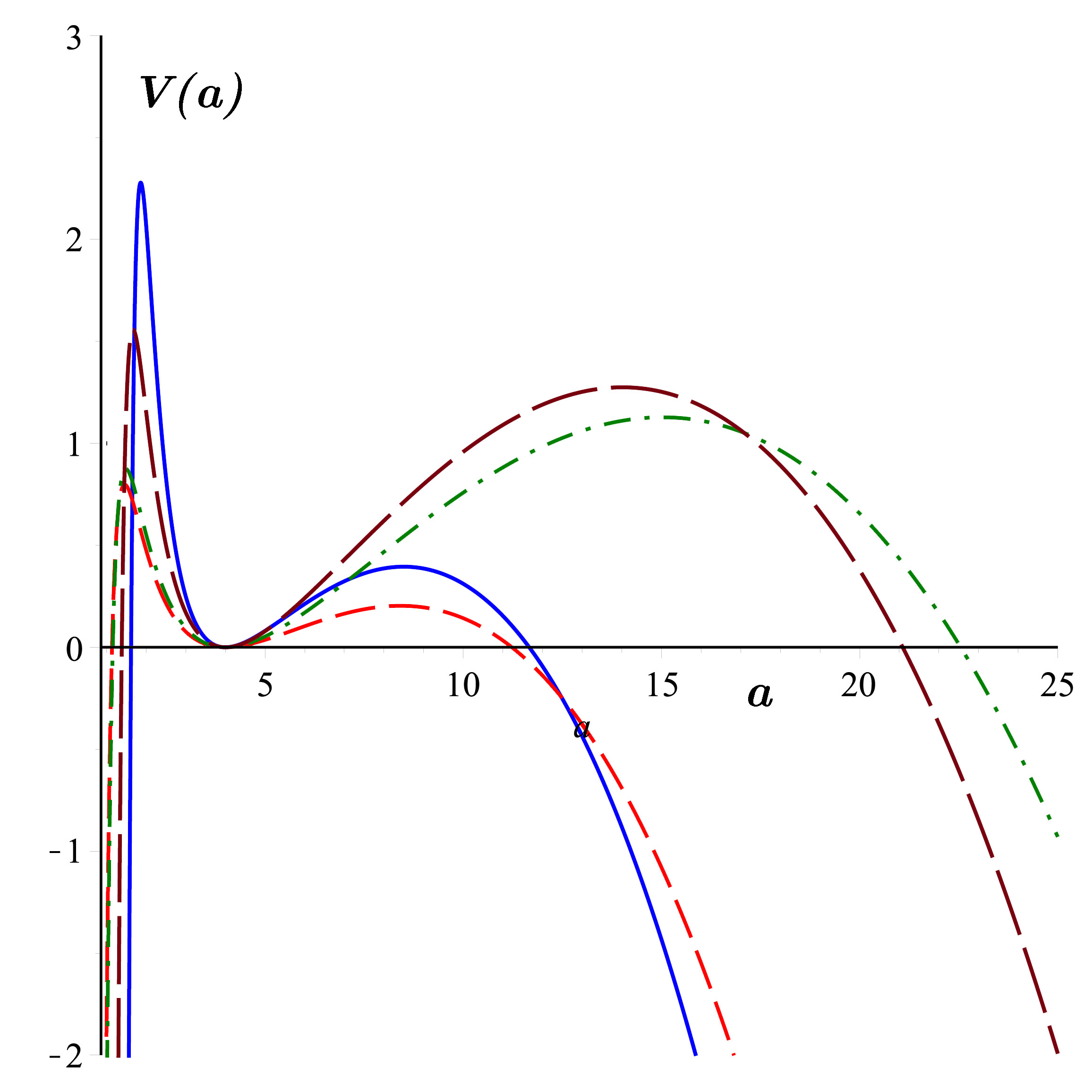
Figure 2: Potential $V\left(a\right)$ versus $a$ for common $r_{+}=1$ and $\ell^{2}=1$ but individually: blue / solid $w=5$, $\alpha=0.2,$ red / short-dash $w=2.7$, $\alpha=0.17,$ green / dash-dot $w=2.7$, $\alpha=0.137$ and brown / long-dash $w=2.7$, $\alpha=0.155.$

One can explicitly show that $V\left(a\right)$ is zero when $a=a_{0}.$ Also its first derivative vanishes at the equilibrium radius but the second derivative is obtained to be

$$V_{0}^{\prime\prime}=\frac{1}{2\left(4-\alpha^{2}\right)\ell^{2}a_{0}^{\alpha^{2}}\left(1-\left(\frac{r_{+}}{a_{0}}\right)^{\frac{4-\alpha^{2}}{2}}\right)}\times\\ \left[4\left(\left(3w+5\right)\alpha^{2}+4w-4\right)\left(\frac{r_{+}}{a_{0}}\right)^{\frac{4-\alpha^{2}}{2}}\right.-\\ \left.\left(\alpha^{2}+4w\right)\left(\alpha^{2}+4\right)\left(\frac{r_{+}}{a_{0}}\right)^{4-\alpha^{2}}-8\alpha^{2}\left(1+w\right)\right].$$ (53)

To have the wormhole locally stable, $V_{0}^{\prime\prime}$ must be positive in the vicinity of $a=a_{0}.$ Before that we note that, $r_{+}$ and $\ell^{2}$ play as scale parameters. In Fig. 1 we present the general behavior of $V_{0}^{\prime\prime}$ in terms of $w$ and $x=\frac{a_{0}}{r_{+}}$ but $0\leq\alpha<2$. In this figure the regions labeled by $S$ are the stable part of the parameters. Also the point $F$ is located at

$$x_{F}=\left(\frac{2\alpha^{2}}{3\alpha^{2}-4}-\frac{2\left(4-\alpha^{2}\right)\alpha}{\left(3\alpha^{2}-4\right)\sqrt{4+\alpha^{2}}}\right)^{\frac{-2}{4-\alpha^{2}}}$$ (54)

with

$$w_{F}=\frac{\left(\alpha^{4}-7\alpha^{2}+4\right)\sqrt{4+\alpha^{2}}+\alpha^{3}\left(4+\alpha^{2}\right)}{\left(5\alpha^{2}+4\right)\sqrt{4+\alpha^{2}}-4\alpha\left(4+\alpha^{2}\right)}.$$ (55)

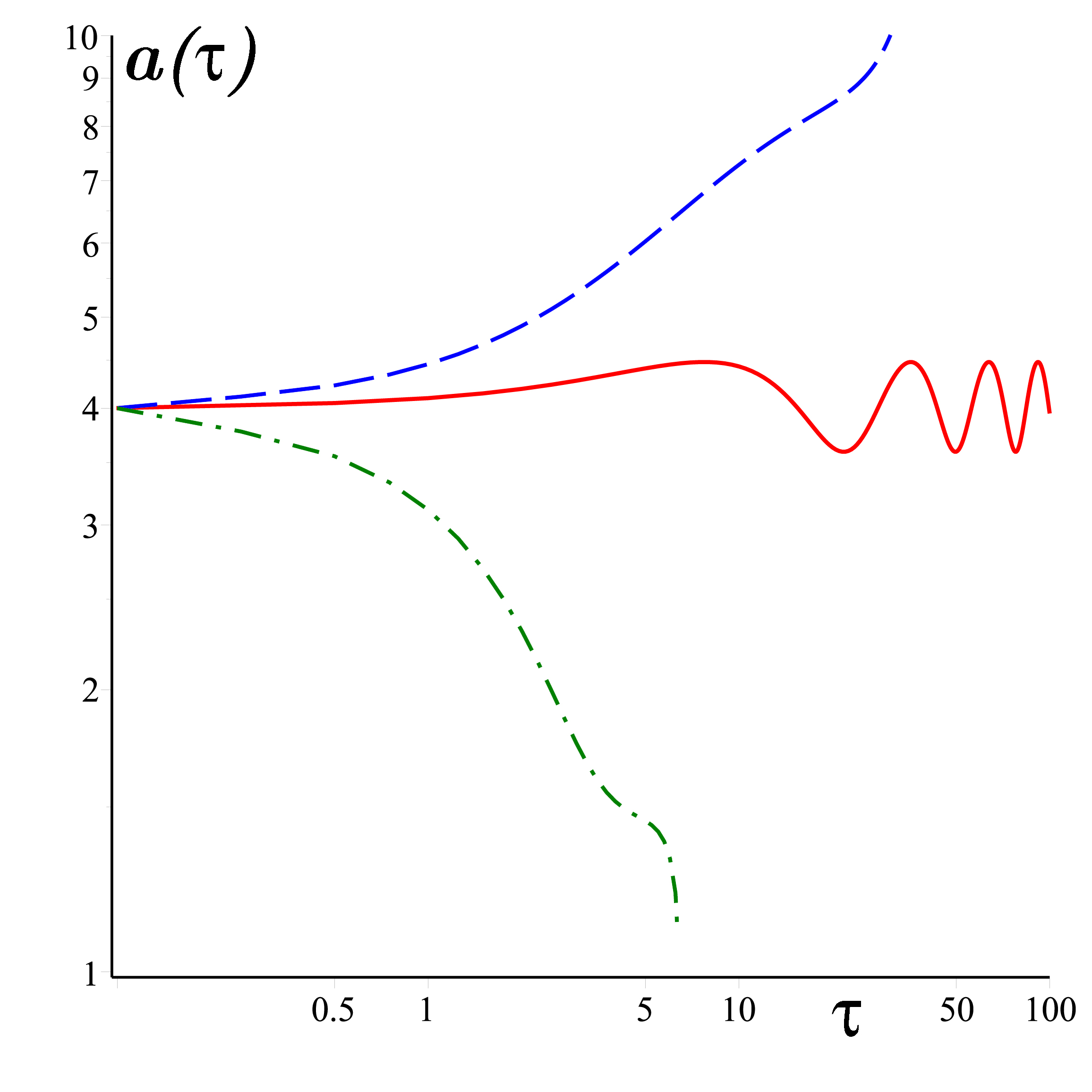
Figure 3: The motion of the throat under the potential shown in Fig. 2 (red/short-dash) with three different possibilities / initial velocity. The axis are logarithmic and dash, solid and dash-dot represent evaporation, oscillation and collapse of the thin-shell wormhole with initial velocities $\left.\frac{da}{d\tau}\right|_{\tau=0}=$ $0.46$, $0.10$ and $-0.895$ respectively.

In addition to that the vertical asymptote is given by $x=x_{a}$ where

$$x_{a}=\left(\frac{4+\alpha^{2}}{2\alpha^{2}}\right)^{\frac{2}{4-\alpha^{2}}}.$$ (56)

This, however, does not mean that the wormhole is stable against any kind of perturbation as a matter of fact, it is valid only for small perturbation. To find the exact motion of the throat after a general perturbation one should solve the general equation of motion either analytically or numerically. In Fig. 2 we plot the potential $V\left(a\right)$ versus $a$ for certain values of parameters which are given in its caption. We observe that for small perturbation $a=a_{0}=4$ is a local stable equilibrium point for all different cases. As a function of proper time the throat radius $a\left(\tau\right)$ is plotted in Fig. (3). It is observed that this provides a stable, i.e. oscillatory radius wormhole within certain range of initial velocities. Fig. (2) justifies explicitly the stability property since the radius is confined in between two high potential barriers.

IV Conclusion

In Einstein’s general relativity wormholes / thin-shell wormholes have two characteristic features that often attract criticism. The first is the occurrence of negative energy density which, with the exception of some alternative works 65 is almost taken for granted while the second concerns about the stability of such structures. Our aim in this paper was to consider Einstein’s gravity solutions with a scalar charge and investigate whether stable wormholes can be established. To this end we presented first an infinite class of solutions with well-known limits. Remarkably it is found that scalar charge ($\alpha$) gives rise to stability regions for the underlying thin-shell wormholes. Small linear perturbation within certain limits of initial velocity is shown to keep the thin-shell wormhole stable. Arbitrary perturbations, expectedly, either collapses or evaporates the wormhole. Not only through perturbations but finely tuned Einstein-Scalar thin-shell wormholes also can be established which are eternally stable in their deep potential well. It is our strong belief that similar results hold also in $3+1-$dimensions, however, the technical details may not be as straightforward as in the present $2+1-$dimensional case.

References

- (1) M. Bañados, C. Teitelboim, J. Zanelli, Phys. Rev. Lett. 69, 1849 (1992).
- (2) M. Bañados, M. Henneaux, C. Teitelboim and J. Zanelli, Phys. Rev. D 48, 1506 (1993).
- (3) C. Martinez, C. Teitelboim and J. Zanelli, Phys. Rev. D 61, 104013 (2000).
- (4) S. Carlip, Quantum Gravity in 2 + 1-Dimensions, Cambridge University Press, 1998.
- (5) S. Carlip, Living Rev. Rel. 8, 1 (2005).
- (6) S. Carlip, Class. Quantum Grav. 12, 2853 (1995).
- (7) J. D. Barrow, A.B. Burd, and D. Lancaster, Class. Quantum Grav. 3, 551 (1986).
- (8) E. Ayón-Beato, A. Garcia, A. Macias, J. Perez-Sanchez, Phys. Lett. B, 495, 164 (2000).
- (9) E. Hirschmann, A. Wang and Y. Wu, Class. Quant. Grav., 21, 1791 (2004);
- (10) H-J. Schmidta and D. Singleton, Phys. Lett. B, 721, 294 (2013).
- (11) S. H. Mazharimousavi and M. Halilsoy, Eur. Phys. J. C 76, 95 (2016).
- (12) S. H. Mazharimousavi and M. Halilsoy, Eur. Phys. J. Plus, 130, 158 (2015).
- (13) L. Zhao, W. Xu, and B. Zhu, Com. Theo. Phys., 61, 475 (2014).
- (14) O. Gurtug, S. Habib Mazharimousavi, and M. Halilsoy, Phys. Rev. D 85, 104004 (2012).
- (15) W. Xu and L. Zhao, Phys. Rev. D 87, 124008 (2013).
- (16) S. Deser and P.O. Mazur, Class. Quantum Grav. 2, L51 (1985).
- (17) P. M. Sa, A. Kleber, and J. P. S. Lemos, Class. Quantum Grav. 13, 125 (1996).
- (18) K. Shiraishi, J. Math. Phys. 34, 1480 (1993).
- (19) D. Park and J. K. Kim, J. Math. Phys. 38, 2616 (1997).
- (20) K. C. K. Chan and R. B. Mann, Phys. Rev. D 50, 6385 (1994).
- (21) K. C. K. Chan and R. B. Mann, Phys. Rev. D 52, 2600 (1995).
- (22) S. Fernando, Phys. Rev. D 79, 124026 (2009).
- (23) S. Fernando, Phys. Lett. B 468, 201 (1999).
- (24) T. Koikawa, T. Maki and A. Nakamula, Phys. Lett. B 414, 45 (1997).
- (25) K. Chan, Phys. Rev. D 55, 3564 (1997).
- (26) P. M. Sá, A. Kleber and J. P. S. Lemos, Class. Quantum Grav. 13, 125 (1996).
- (27) S. H. Mazharimousavi and M. Halilsoy, Eur. Phys. J. C, 76, 458 (2016).
- (28) R. Yamazaki and D. Ida, Phys. Rev. D 64, 024009 (2001).
- (29) Ó. Dias and J. Lemos, Phys. Rev. D 64, 064001 (2001).
- (30) M. Visser, Phys. Rev. D 39, 3182 (1989).
- (31) M. Visser, Nucl. Phys. H 328, 203 (1989).
- (32) M. S. Morris and K. S. Thorne, Am. J. Phys. 56, 395 (1988).
- (33) M. S. Morris, K. S. Thorne and U. Yurtsever, Phys. Rev. Lett. 61, 1446 (1988).
- (34) M. Visser, Lorentzian Wormholes: from Einstein to Hawoking (American Institute of Physics, New York, 1995).
- (35) E. Poisson and M. Visser, Phys. Rev. D 52, 7318 (1995).
- (36) P. Musgrave and K. Lake, Class. Quantum Grav. 13, 1885 (1996).
- (37) P. Musgrave and K. Lake, Class. Quantum Grav. 14, 1285 (1997).
- (38) S. C. Davis, Phys. Rev. D 67, 024030 (2003).
- (39) E. F. Eiroa and C. Simeone, Phys. Rev. D 70, 044008 (2004).
- (40) E. F. Eiroa and C. Simeone, Phys. Rev. D 71, 127501 (2005).
- (41) F. Lobo, Phys. Rev. D 71, 124022 (2005).
- (42) F. Lobo, Phys. Rev. D 73, 064028 (2006).
- (43) F. Rahaman, M. Kalam and S. Chakraborty, Gen. Relativ. Gravit., 38, 1687 (2006).
- (44) M. Thibeault, C. Simeone and E. F. Eiroa, Gen. Relativ. Gravit. 38, 1593 (2006).
- (45) M. G. Richarte and C. Simeone, Phys. Rev. D 76, 087502 (2007).
- (46) M. G. Richarte and C. Simeone, Phys. Rev. D 77, 089903 (2008).
- (47) E. F. Eiroa, M. G. Richarte and C. Simeone, Phys. Lett. A 373, 1 (2008).
- (48) T. Bandyopadhyay and S. Chakraborty, Class. Quantum Grav., 26, 085005 (2009).
- (49) S. H. Mazharimousavi, M. Halilsoy and Z. Amirabi, Class. Quantum Grav., 28, 025004 (2011).
- (50) P. E. Kashargin and S. V. Sushkov, Gravit. Cosmol. 17, 119 (2011).
- (51) F. Rahaman, A. Banerjee and I. Radinschi, Int. J Theor. Phys., 51, 1680 (2012).
- (52) A. Banerjee, Int. J Theor. Phys., 52, 2943 (2013).
- (53) S. H. Mazharimousavi, M. Halilsoy and Z. Amirabi, Phys. Rev. D 89, 084003 (2014).
- (54) S. H. Mazharimousavi and M. Halilsoy, Eur. Phys. J. C 74, 3073 (2014).
- (55) C. Bejarano, E. F. Eiroa and C. Simeone, Eur. Phys. J. C 74, 3015 (2014).
- (56) S. H. Mazharimousavi and M. Halilsoy, Eur. Phys. J. C 75, 81 (2015).
- (57) J. D. Brown and J. W. York, Phys. Rev. D 47, 1407 (1993).
- (58) J. D. Brown, J. Creighton and R. B. Mann, Phys. Rev. D 50, 6394 (1994).
- (59) L. Fatibene, M. Ferraris, M. Francaviglia and M. Raiteri, Phys. Rev. D 60, 124012 (1999).
- (60) L. Fatibene, M. Ferraris, M. Francaviglia and M. Raiteri, Phys. Rev. D 60, 124013 (1999).
- (61) L. Fatibene, M. Ferraris, M. Francaviglia and M. Raiteri, J. Math. Phys. 42, 1173 (2001).
- (62) G. Darmois 1927 Mémorial de Sciences Mathématiques, Fascicule XXV Les equations de la gravitation einsteinienne ch V.
- (63) W. Israel, Nuovo Cimento B 44, 1 (1966).
- (64) W. Israel, Nuovo Cimento B 48, 463 (1966).
- (65) S. H. Mazharimousavi and M. Halilsoy, Eur. Phys. J. C 47, 3067 (2014).