DYNAMICS OF BOSE-EINSTEIN CONDENSATE WITH ACCOUNT OF PAIR CORRELATIONS

Abstract

The system of dynamic equations for Bose-Einstein condensate at zero temperature with account of pair correlations is obtained. The spectrum of small oscillations of the condensate in a spatially homogeneous state is explored. It is shown that this spectrum has two branches: the sound wave branch and the branch with an energy gap.
Key words: Bose-Einstein condensate, anomalous and normal averages, pair correlations, sound branch of elementary excitations, elementary excitations with energy gap.

I Introduction

Bose-Einstein condensate of a low-density system of weakly interacting Bose particles at zero temperature is usually described by the Gross-Pitaevskii equation Gross61 ; Pit61 , which is nowadays widely used for study of the condensates created in magnetic and laser traps PitStr03 ; PitSm02 . The Gross-Pitaevskii equation is obtained in the self-consistent field approximation, where the short-range correlations between particles are neglected. In this case, the Bose system is described in terms of the coherent state vectorYuM11 . Meanwhile, the consideration of the pair correlations, being essential at short distances, turns out to be important even for systems with low densities since it leads to some qualitatively new results. For example, in a dilute classical gas the account for pair correlations allows us to obtain the integral of collisions in the kinetic equation and, therefore, all effects which are described by the Boltzmann equation Bog70 .

In the present work, we obtain the system of dynamical equations in the approximation in which besides the one-particle anomalous averages, the two-particle correlations are also taken into account but the correlations of more number of particles are neglected. Small oscillations on the background of a spatially homogeneous equilibrium state are studied. It is shown that when considering pair correlations in Bose-Einstein condensate, there exist two branches of elementary excitations. One of them is acoustic, another one has an energy gap in the long wavelength limit.    

II Equations for averages of the field operators

An arbitrary operator in the Heisenberg representation $A=e^{i\frac{H}{\hbar}}A(0)e^{-i\frac{H}{\hbar}}$ satisfies the dynamic equation

$$\begin{array}[]{ll}\displaystyle{i\hbar\frac{\partial A}{\partial t}=[H,A],}\end{array}$$ (1)

where in the second-quantized representation the Hamiltonian can be written as a sum of operators of the kinetic energy and the energy of pair interaction $H=H_{1}+H_{2}$,

$$\begin{array}[]{ll}\displaystyle{H_{1}=\int d{\bf r}_{1}d{\bf r}_{2}H({\bf r}_{1},{\bf r}_{2})\Psi^{\dagger}({\bf r}_{1},t)\Psi({\bf r}_{2},t),\vspace{2mm}}\\ \displaystyle{\hskip 99.58464ptH_{2}=\vspace{2mm}}\\ \displaystyle{=\!\frac{1}{2}\!\int\!\!d{\bf r}_{1}d{\bf r}_{2}U(|{\bf r}_{1}-{\bf r}_{2}|)\Psi^{\dagger}({\bf r}_{1},t)\Psi^{\dagger}({\bf r}_{2},t)\Psi({\bf r}_{2},t)\Psi({\bf r}_{1},t).}\end{array}$$ (2)

Here

$$\begin{array}[]{ll}\displaystyle{H({\bf r}_{1},{\bf r}_{2})=-\frac{\hbar^{2}}{2m}\Delta_{1}\delta({\bf r}_{1}-{\bf r}_{2})+[U_{0}({\bf r}_{1})-\mu]\delta({\bf r}_{1}-{\bf r}_{2}),}\end{array}$$ (3)

$m$ is the bose-particle mass, $U_{0}({\bf r})$ – the energy of particle in the external field, $U(|{\bf r}_{1}-{\bf r}_{2}|)$ – the particle interaction potential. The field operators satisfy the usual commutation relations. Let $\langle\Psi\rangle$ is the average of field operator. Then we can write down our field operator separating the $c$-number and operator parts:

$$\begin{array}[]{ll}\displaystyle{\Psi=\langle\Psi\rangle+\xi,\;\;\;\Psi^{\dagger}=\langle\Psi\rangle^{*}+\xi^{*},}\end{array}$$ (4)

The operator part is defined so that it meets the obvious relations:

$$\begin{array}[]{ll}\displaystyle{\langle\xi\rangle=\langle\xi^{\dagger}\rangle=0.}\end{array}$$ (5)

Here the averaging is implied in the sense of the quasiaverages for systems with broken phase symmetry Bog71 ; YuM97 . We will assume that the normal averages, which are invariant under the phase transformation of the field operators $\Psi\rightarrow\Psi^{\prime}=e^{i\alpha}\Psi$, and the anomalous averages, where this invariance is broken, are both nonzero. It is to be noted that the property of superfluidity is connected with just the existence of these anomalous averages.

We introduce the the following notation for the anomalous average of the field operator

$$\begin{array}[]{ll}\displaystyle{\eta({\bf r},t)=\langle\Psi({\bf r},t)\rangle,\;\;\eta^{*}=\langle\Psi^{\dagger}({\bf r},t)\rangle.}\end{array}$$ (6)

The averages of the products of several field operators can be written in terms of the averages of the products of operators $\xi,\xi^{\dagger}$, which will be called as the overcondensate operators . For example, for the case of two field operators, using Eq.(5), we have

$$\begin{array}[]{ll}\displaystyle{\langle\Psi^{\dagger}({\bf r})\Psi({\bf r}^{\prime})\rangle=\eta^{*}({\bf r})\eta({\bf r}^{\prime})+\langle\xi^{\dagger}({\bf r})\xi({\bf r}^{\prime})\rangle,\vspace{2mm}}\\ \displaystyle{\langle\Psi({\bf r})\Psi({\bf r}^{\prime})\rangle=\eta({\bf r})\eta({\bf r}^{\prime})+\langle\xi({\bf r})\xi({\bf r}^{\prime})\rangle,\vspace{2mm}}\\ \displaystyle{\langle\Psi^{\dagger}({\bf r})\Psi^{\dagger}({\bf r}^{\prime})\rangle=\eta^{*}({\bf r})\eta^{*}({\bf r}^{\prime})+\langle\xi^{\dagger}({\bf r})\xi^{\dagger}({\bf r}^{\prime})\rangle.}\end{array}$$ (7)

Similarly, we can write down the averages of a greater number of field operators. They will also contain the averages of a greater number of the overcondensate operators of the form $\langle\xi^{\dagger}({\bf r}_{1})\xi^{\dagger}({\bf r}_{2})\xi({\bf r}_{3})\rangle$, $\langle\xi^{\dagger}({\bf r}_{2})\xi^{\dagger}({\bf r}_{3})\xi^{\dagger}({\bf r}_{4})\rangle$, $\langle\xi^{\dagger}({\bf r}_{1})\xi^{\dagger}({\bf r}_{2})\xi^{\dagger}({\bf r}_{3})\xi^{\dagger}({\bf r}_{4})\rangle$ and etc. Setting successively the operator $A$ in the Heisenberg equation (1) equal to $\Psi^{\dagger}\Psi$, $\Psi\Psi$, $\Psi^{\dagger}\Psi^{\dagger},\ldots\,$ and carrying out averaging, we will get the infinite chain of coupled equations for the averages $\langle\Psi\rangle$, $\langle\Psi^{\dagger}\Psi\rangle$, $\langle\Psi\Psi\rangle$, $\langle\Psi^{\dagger}\Psi^{\dagger}\rangle\ldots\,$, which is similar to the Bogoliubov-Born-Green-Kirkwood-Yvon chain [6] in the kinetic theory of classical gases.

So, the equation for the average of the field operator (6) has the form:

$$\begin{array}[]{ll}\displaystyle{i\hbar\frac{\partial\eta({\bf r})}{\partial t}=\int H({\bf r},{\bf r}^{\prime\prime})\eta({\bf r}^{\prime\prime})d{\bf r}^{\prime\prime}+\vspace{2mm}}\\ \displaystyle{\hskip 39.83385pt+\int U(|{\bf r}-{\bf r}^{\prime\prime}|)\langle\Psi^{\dagger}({\bf r}^{\prime\prime})\Psi({\bf r}^{\prime\prime})\Psi({\bf r})\rangle d{\bf r}^{\prime\prime}.}\end{array}$$ (8)

and the equations for the normal and anomalous pair-wise correlations are written as follows

$$\begin{array}[]{ll}\displaystyle{i\hbar\frac{\partial\langle\Psi^{\dagger}({\bf r})\Psi({\bf r}^{\prime})\rangle}{\partial t}=\vspace{2mm}}\\ \displaystyle{\!=\!\!\int\!\!\Big{[}H\!({\bf r}^{\prime}\!,{\bf r}^{\prime\prime})\langle\Psi^{\dagger}\!({\bf r})\Psi({\bf r}^{\prime\prime})\rangle-\!H^{*}\!({\bf r},{\bf r}^{\prime\prime})\langle\Psi^{\dagger}\!({\bf r}^{\prime\prime})\Psi({\bf r}^{\prime})\rangle\Big{]}d{\bf r}^{\prime\prime}-\vspace{2mm}}\\ \displaystyle{-\int\!\Big{[}U(|{\bf r}-{\bf r}^{\prime\prime}|)-U(|{\bf r}^{\prime}-{\bf r}^{\prime\prime}|)\Big{]}\times\vspace{2mm}}\\ \displaystyle{\hskip 88.20354pt\times\langle\Psi^{\dagger}({\bf r})\Psi^{\dagger}({\bf r}^{\prime\prime})\Psi({\bf r}^{\prime\prime})\Psi({\bf r}^{\prime})\rangle\,d{\bf r}^{\prime\prime},}\end{array}$$ (9)

$$\begin{array}[]{ll}\displaystyle{i\hbar\frac{\partial\langle\Psi({\bf r})\Psi({\bf r}^{\prime})\rangle}{\partial t}=\vspace{2mm}}\\ \displaystyle{=\!\int\!\!\Big{[}H\!({\bf r},{\bf r}^{\prime\prime})\langle\Psi({\bf r}^{\prime})\Psi({\bf r}^{\prime\prime})\rangle+\!H\!({\bf r}^{\prime},{\bf r}^{\prime\prime})\langle\Psi({\bf r})\Psi({\bf r}^{\prime\prime})\rangle\Big{]}d{\bf r}^{\prime\prime}+\vspace{2mm}}\\ \displaystyle{+\,U({\bf r},{\bf r}^{\prime})\langle\Psi({\bf r})\Psi({\bf r}^{\prime})\rangle\,-\vspace{2mm}}\\ \displaystyle{-\int\!\Big{[}U(|{\bf r}-{\bf r}^{\prime\prime}|)+U(|{\bf r}^{\prime}-{\bf r}^{\prime\prime}|)\Big{]}\times\vspace{2mm}}\\ \displaystyle{\hskip 85.35826pt\times\langle\Psi^{\dagger}({\bf r}^{\prime\prime})\Psi^{\dagger}({\bf r}^{\prime\prime})\Psi({\bf r})\Psi({\bf r}^{\prime})\rangle\,d{\bf r}^{\prime\prime}.}\end{array}$$ (10)

In the following we will describe the condensate by using the one-particle averages (6) and restrict ourselves to considering only pair correlations of the overcondensate operators introduced by relations (4), having defined the following correlation functions:

$$\begin{array}[]{ll}\displaystyle{g({\bf r},{\bf r}^{\prime},t)=\langle\xi^{\dagger}({\bf r},t)\xi({\bf r}^{\prime},t)\rangle,\vspace{2mm}}\\ \displaystyle{\tau({\bf r},{\bf r}^{\prime},t)=\langle\xi({\bf r},t)\xi({\bf r}^{\prime},t)\rangle,\vspace{2mm}}\\ \displaystyle{\tau^{*}({\bf r},{\bf r}^{\prime},t)=\langle\xi^{\dagger}({\bf r},t)\xi^{\dagger}({\bf r}^{\prime},t)\rangle.\vspace{2mm}}\\ \end{array}$$ (11)

The averages of a greater number of the overcondensate operators will be neglected that seems to be acceptable for sufficiently diluted systems. Functions (11) have the obvious symmetry properties

$$\begin{array}[]{ll}\displaystyle{g({\bf r},{\bf r}^{\prime},t)=g^{*}({\bf r}^{\prime},{\bf r},t),\;\tau({\bf r},{\bf r}^{\prime},t)=\tau({\bf r}^{\prime},{\bf r},t),\vspace{2mm}}\\ \displaystyle{\hskip 56.9055pt\tau^{*}({\bf r},{\bf r}^{\prime},t)=\tau^{*}({\bf r}^{\prime},{\bf r},t).}\end{array}$$ (12)

When only the pair correlations are taken into account, from (8) – (10) one can get the closed system of equations for functions $\eta({\bf r},t)$ $g({\bf r},{\bf r}^{\prime},t)$ $\tau({\bf r},{\bf r}^{\prime},t)$

$$\begin{array}[]{ll}\displaystyle{i\hbar\frac{\partial\eta({\bf r})}{\partial t}=-\frac{\hbar^{2}}{2m}\Delta\eta({\bf r})+[U_{0}({\bf r})-\mu]\eta({\bf r})+\vspace{2mm}}\\ \displaystyle{+\int U(|{\bf r}-{\bf r}^{\prime\prime}|)\Big{[}|\eta({\bf r}^{\prime\prime})|^{2}\eta({\bf r})+\eta^{*}({\bf r}^{\prime\prime})\tau({\bf r},{\bf r}^{\prime\prime})+\vspace{2mm}}\\ \hskip 42.67912pt+\eta({\bf r}^{\prime\prime})g^{*}({\bf r},{\bf r}^{\prime\prime})+\eta({\bf r})g({\bf r}^{\prime\prime},{\bf r}^{\prime\prime})\Big{]},\end{array}$$ (13)

$$\begin{array}[]{ll}\displaystyle{i\hbar\frac{\partial\tau({\bf r},{\bf r}^{\prime})}{\partial t}=U(|{\bf r}-{\bf r}^{\prime}|)\eta({\bf r})\eta({\bf r}^{\prime})+U(|{\bf r}-{\bf r}^{\prime}|)\tau({\bf r},{\bf r}^{\prime})-\vspace{2mm}}\\ \displaystyle{-\frac{\hbar^{2}}{2m}(\Delta+\Delta^{\prime})\tau({\bf r},{\bf r}^{\prime})+[U_{0}({\bf r})+U_{0}({\bf r}^{\prime})-2\mu]\tau({\bf r},{\bf r}^{\prime})+\vspace{2mm}}\\ \displaystyle{+\!\int\!\!d{\bf r}^{\prime\prime}U(|{\bf r}-{\bf r}^{\prime\prime}|)\Big{[}|\eta({\bf r}^{\prime\prime})|^{2}\tau({\bf r},{\bf r}^{\prime})+\eta({\bf r})\eta^{*}({\bf r}^{\prime\prime})\tau({\bf r}^{\prime},{\bf r}^{\prime\prime})+\vspace{2mm}}\\ \displaystyle{+\,\eta({\bf r})\eta({\bf r}^{\prime\prime})g({\bf r}^{\prime\prime},{\bf r}^{\prime})\Big{]}\!+\!\int\!\!d{\bf r}^{\prime\prime}U(|{\bf r}^{\prime}-{\bf r}^{\prime\prime}|)\Big{[}|\eta({\bf r}^{\prime\prime})|^{2}\tau({\bf r},{\bf r}^{\prime})+\vspace{2mm}}\\ \displaystyle{\hskip 39.83385pt+\,\eta({\bf r}^{\prime})\eta^{*}({\bf r}^{\prime\prime})\tau({\bf r},{\bf r}^{\prime\prime})+\eta({\bf r}^{\prime})\eta({\bf r}^{\prime\prime})g({\bf r}^{\prime\prime},{\bf r})\Big{]},}\end{array}$$ (14)

$$\begin{array}[]{ll}\displaystyle{i\hbar\frac{\partial g({\bf r},{\bf r}^{\prime})}{\partial t}\!=\!\frac{\hbar^{2}}{2m}(\Delta-\!\Delta^{\prime})g({\bf r},{\bf r}^{\prime})-\![U_{0}({\bf r})\!-\!U_{0}({\bf r}^{\prime}\!)]g({\bf r},{\bf r}^{\prime})-\vspace{2mm}}\\ \displaystyle{-\int\!d{\bf r}^{\prime\prime}U(|{\bf r}-{\bf r}^{\prime\prime}|)\Big{[}|\eta({\bf r}^{\prime\prime})|^{2}g({\bf r},{\bf r}^{\prime})+\eta^{*}({\bf r})\eta({\bf r}^{\prime\prime})g({\bf r}^{\prime\prime},{\bf r}^{\prime})+\vspace{2mm}}\\ \displaystyle{+\eta^{*}\!({\bf r})\eta^{*}\!({\bf r}^{\prime\prime})\tau({\bf r}^{\prime\prime},{\bf r}^{\prime})\Big{]}\!+\!\!\int\!\!d{\bf r}^{\prime\prime}U(|{\bf r}^{\prime}-{\bf r}^{\prime\prime}|)\Big{[}|\eta({\bf r}^{\prime\prime})|^{2}g({\bf r},{\bf r}^{\prime})+\vspace{2mm}}\\ \displaystyle{\hskip 39.83385pt+\eta({\bf r}^{\prime})\eta^{*}({\bf r}^{\prime\prime})g({\bf r},{\bf r}^{\prime\prime})+\eta({\bf r}^{\prime})\eta({\bf r}^{\prime\prime})\tau^{*}({\bf r}^{\prime\prime},{\bf r})\Big{]}.}\end{array}$$ (15)

One should note that this system of equations is invariant under time-reversal transformation, because along with solutions $\eta({\bf r},t)$, $g({\bf r},{\bf r}^{\prime},t)$, $\tau({\bf r},{\bf r}^{\prime},t)$ it also has the solutions $\eta^{*}({\bf r},-t)$, $g^{*}({\bf r},{\bf r}^{\prime},-t)$, $\tau^{*}({\bf r},{\bf r}^{\prime},-t)$. Neglecting the pair correlations $\tau({\bf r},{\bf r}^{\prime},t)$ and $g({\bf r},{\bf r}^{\prime},t)$, equation (13) takes the form of the Gross-Pitaevskii equation [1,2]. In what follows, where it will not cause confusion, as in equations (13) – (15), for brevity the explicit time-dependance of the averages will be omitted.

The average of the operator of the total number of particles $N$ is given by the formula

$$\langle N\rangle=\int d{\bf r}[\eta^{*}({\bf r},t)\eta({\bf r},t)+g({\bf r},{\bf r},t)],$$ (16)

and the particle number density is, obviously, $n({\bf r},t)=\eta^{*}({\bf r},t)\eta({\bf r},t)+g({\bf r},{\bf r},t)$.

III Local form of equations

Equations (13) – (15) are integro-differential. While studying the states that slowly vary on the scales comparable to characteristic radius $r_{0}$ of action of the interparticle interaction potential $U(|{\bf r}-{\bf r^{\prime}}|)$, we can pass to differential equations. The pair correlation functions (11) depend on two coordinates ${\bf r},{\bf r}^{\prime}$. It is convenient to introduce new variables $\vec{\rho}={\bf r}-{\bf r}^{\prime}$, ${\bf R}=\frac{1}{2}({\bf r}+{\bf r}^{\prime})$, then

$$\begin{array}[]{ll}\displaystyle{\tau({\bf r},{\bf r}^{\prime})=\tau\big{(}{\bf R}+\frac{\vec{\rho}}{2},{\bf R}-\frac{\vec{\rho}}{2}\big{)}\equiv\tau({\bf R},\vec{\rho}),\vspace{2mm}}\\ \displaystyle{g({\bf r},{\bf r}^{\prime})=g\big{(}{\bf R}+\frac{\vec{\rho}}{2},{\bf R}-\frac{\vec{\rho}}{2}\big{)}\equiv g({\bf R},\vec{\rho}).}\end{array}$$ (17)

These functions slowly change depending on the pair’s center-mass coordinate ${\bf R}$ on distances of the order of the interparticle potential radius $r_{0}$. The correlation functions can be presented in the form:

$${\tau({\bf R},\vec{\rho})=\sum_{\bf k}\tau_{{\bf k}}({\bf R})e^{i{\bf k}\vec{\rho}},\;\;g({\bf R},\rho)=\sum_{\bf k}g_{{\bf k}}({\bf R})e^{i{\bf k}\vec{\rho}}.}$$ (18)

In the following, only the term with ${\bf k}=0$ will be taken into account in these sums. It means that instead of the exact functions $\tau({\bf R},\rho)$ $g({\bf R},\rho)$, we will use the functions which are averaged over a macroscopic volume $V_{0}\sim L^{3}$, where $L\gg r_{0}$:

$${\tau_{0}({\bf R})\approx V_{0}^{-1}\!\int\!\tau({\bf R},\vec{\rho})\,d\vec{\rho},\;\;g_{0}({\bf R})\approx V_{0}^{-1}\!\int\!g({\bf R},\vec{\rho})\,d\vec{\rho}.}$$

This approximation is acceptable if one considers perturbations on spatial scales that significantly exceed the radius of action of the interparticle potential.

It is worth noting that in obtained equations the behavior of the interparticle interaction potential at short distances plays an important role. The form of the potential is poorly known here. Moreover, for many model potentials such as, for example the Lennard-Jones potential, it is assumed that at short distances it goes to infinity. Note also that the use of model potentials which go to infinity at short distances in some cases leads to considerable difficulties, because such potentials do not have the Fourier representation. Meanwhile, the requirement of “impermeability” of atoms at arbitrary high pressures is very strict, since there should exist a pressure at which an atom will be “crushed” and stop existing as a separate structural unit. Therefore, in our opinion, it is physically reasonable and natural to use the potentials, which take a finite value at short distances. It should also be noted that the quantum-chemical calculations give potentials with a finite, albeit large, value at zero Aziz91 ; And93 .

In this local approximation, the system of equations (13) – (15) takes the form:

$$\begin{array}[]{ll}\displaystyle{i\hbar\frac{\partial\eta({\bf r})}{\partial t}=-\frac{\hbar^{2}}{2m}\Delta\eta({\bf r})+[U_{0}({\bf r})-\mu]\eta({\bf r})+\vspace{2mm}}\\ \displaystyle{+U_{0}\left[|\eta({\bf r})|^{2}\eta({\bf r})+\eta^{*}({\bf r})\tau({\bf r})+2\eta({\bf r})g({\bf r})\right],}\end{array}$$ (19)

$$\begin{array}[]{ll}\displaystyle{i\hbar\frac{\partial\tau({\bf r})}{\partial t}=-\frac{\hbar^{2}}{4m}\Delta\tau({\bf r})+U(0)\eta^{2}({\bf r})+U(0)\tau({\bf r})\,+\vspace{2mm}}\\ \displaystyle{+\,[2U_{0}({\bf r})-2\mu]\tau({\bf r})+U_{0}\!\left[4|\eta({\bf r})|^{2}\tau({\bf r})+2\eta^{2}({\bf r})g({\bf r})\right],}\end{array}$$ (20)

$$\begin{array}[]{ll}\displaystyle{i\hbar\frac{\partial g({\bf r})}{\partial t}=-U_{0}\left[\eta^{*2}({\bf r})\tau({\bf r})-\eta^{2}({\bf r})\tau^{*}(\bf{r})\right].\vspace{2mm}}\end{array}$$ (21)

Here we used the designations: $\tau({\bf R})\equiv\tau({\bf r})$, $g_{0}({\bf R})\equiv g({\bf r})$, $U_{0}\equiv\int U({\bf r})d{\bf r}$. Since the magnitude of the potential energy of interaction of atoms at short distances $U(0)$ is poorly known, it will be regarded as a phenomenological adjustable parameter. For specific calculations we will use a simple model potential of “semi-transparent sphere” form:

$${U({\bf r})=\begin{cases}u,\;\;\;\;\;\;\;r<r_{0}\,,\\ 0,\;\;\;\;\;\;\;r>r_{0}\,.\end{cases}}$$ (22)

The parameter $u$ is assumed to be positive. In this case $U(0)=u$, $U_{0}=uv$, where $v\equiv\frac{4\pi}{3}r_{0}^{3}$ is the ”atomic volume”. The potential (22) has earlier been used in the studies of the Bose systems (see e.g. Brak64 ). Further, we will analyze the system of equations (19) – (21) and use the potential (22) for some estimations.

IV Equilibrium spatially homogeneous state

In this section we will consider the equilibrium state of a spatially homogeneous system. In this case, the functions $\eta({\bf r})\equiv\eta$, $\tau({\bf r})\equiv\tau$, $g({\bf r})\equiv g$ do not depend on coordinates and time. For sufficiently weak interaction, the most of particles will be in the single-particle condensate at zero temperature  Bog47 ; Bog84 . Therefore, we will assume the normal correlation function $g=0$ at the equilibrium state, so that the equilibrium particle number density $n=|\eta|^{2}$. Then, in the absence of the external field, from (19) – (21) there follow the equations which determine the equilibrium state of the system:

$${-\mu\eta+U_{0}\left[|\eta|^{2}\eta+\eta^{*}\tau\right]=0,}$$ (23)

$${U(0)\eta^{2}+\left[U(0)-2\mu+4U_{0}|\eta|^{2}\right]\tau=0,}$$ (24)

$${\eta^{*2}\tau-\eta^{2}\tau^{*}=0.}$$ (25)

Let’s write down the complex quantities extracting their moduli and phases: $\eta=\eta_{0}e^{i\alpha}$, $\tau=\tau_{0}e^{i\beta}$. From (25) it follows that $\sin{(2\alpha-\beta)}=0$. Thus, there are two possibilities $2\alpha-\beta=0$ or $2\alpha-\beta=\pi$. We have to choose the second possibility, since only in this case equations (23),(24) have the physically correct solutions:

$${\eta_{0}\left[\mu-U_{0}(\eta_{0}^{2}-\tau_{0})\right]=0,}$$ (26)

$${U(0)\eta_{0}^{2}-\left[U(0)+4U_{0}\eta_{0}^{2}-2\mu\right]\tau_{0}=0.}$$ (27)

With this choice of phase $\tau=-\tau_{0}e^{2i\alpha}$. After eliminating the chemical potential $\mu$ from these equations, we get

$${\left[U(0)-2U_{0}\tau_{0}\right]\eta_{0}^{2}-[U(0)+2U_{0}\tau_{0}]\tau_{0}=0.}$$ (28)

Note that there does not exist the solution for the system of equations (26) and (27) such that only the single-particle condensate exists $\eta_{0}\neq 0$ and the pair condensate is absent $\tau_{0}=0$. This feature of the Bose systems has been earlier pointed out YuM07 . From (28) it follows the relation between density and the pair correlation:

$${n\equiv\eta_{0}^{2}=\frac{1+2v\tau_{0}}{1-2v\tau_{0}}\tau_{0}.}$$ (29)

Here we have used the relation $U_{0}=uv$ ($v$ is the “atomic volume”), which was obtained above for the potential (22). Hence it follows the restriction $v\tau_{0}<1/2$. The chemical potential

$${\mu=4uv\frac{v\tau_{0}^{2}}{1-2v\tau_{0}}}$$ (30)

proves to be positive. The dependence of the pair correlation on the particle density is given by the relation

$${\tau_{0}v=\frac{1}{2}\left[\sqrt{\left(nv+\frac{1}{2}\right)^{2}+2nv}-\left(nv+\frac{1}{2}\right)\right].}$$ (31)

Here $nv=v/\Omega$, where $\Omega$ is the volume per one particle. In a dilute system $\Omega\gg v$ and $nv\ll 1$. In this case $n\approx\tau_{0}$.

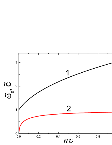
Figure 1: Dependencies of the homogeneous oscillations frequency $\tilde{\omega}_{0}=\omega_{0}/u$ (curve 1) and the speed of sound $\tilde{c}=c/c_{B}$ (curve 2) on density, $c_{B}=\sqrt{uvn/m}$.

V SPECTRUM OF Elementary excitations

In this section we will consider the propagation of small perturbations in a spatially homogeneous system. Setting

$${\eta({\bf r},t)=\eta_{0}+\delta\eta({\bf r},t),\;\tau({\bf r},t)=\tau_{0}+\delta\tau,\;g({\bf r},t)\!=\delta g({\bf r},t),}$$ (32)

we get from (19) – (21) the system of linearized equations:

$$\begin{array}[]{ll}\displaystyle{i\hbar\frac{\partial\delta\eta}{\partial t}=-\frac{\hbar^{2}}{2m}\Delta\delta\eta+U_{0}\Big{[}\left(\eta_{0}^{2}+\tau_{0}\right)\delta\eta+(\eta_{0}^{2}-\tau_{0})\delta\eta^{*}+\vspace{2mm}}\\ \displaystyle{\hskip 99.58464pt+\,\eta_{0}\delta\tau+2\eta_{0}\delta g\Big{]},}\end{array}$$ (33)

$$\begin{array}[]{ll}\displaystyle{i\hbar\frac{\partial\delta\tau}{\partial t}=-\frac{\hbar^{2}}{4m}\Delta\delta\tau+\Big{[}U(0)+2U_{0}(\eta_{0}^{2}+\tau_{0})\Big{]}\delta\tau+\vspace{2mm}}\\ \displaystyle{+\,2\Big{[}U(0)-2U_{0}\tau_{0}\Big{]}\eta_{0}\delta\eta-4U_{0}\eta_{0}\tau_{0}\delta\eta^{*}+2U_{0}\eta_{0}^{2}\delta g,}\end{array}$$ (34)

$$\begin{array}[]{ll}\displaystyle{i\hbar\frac{\partial\delta g}{\partial t}=-U_{0}\Big{[}\eta_{0}^{2}(\delta\tau-\delta\tau^{*})+2\eta_{0}\tau_{0}(\delta\eta-\delta\eta^{*})\Big{]}.}\end{array}$$ (35)

It is convenient to pass from the complex variables $\delta\eta({\bf r},t)$, $\delta\tau({\bf r},t)$, $\delta g({\bf r},t)$ to the real ones

$$\begin{array}[]{ll}\displaystyle{\delta\Psi({\bf r},t)=\delta\eta({\bf r},t)+\delta\eta^{*}({\bf r},t),\vspace{2mm}}\\ \displaystyle{\delta\Phi({\bf r},t)=i\big{[}\delta\eta({\bf r},t)-\delta\eta^{*}({\bf r},t)\big{]},\vspace{2mm}}\\ \displaystyle{\delta\Theta({\bf r},t)=\delta\tau({\bf r},t)+\delta\tau^{*}({\bf r},t),\vspace{2mm}}\\ \displaystyle{\delta\Lambda({\bf r},t)=i\big{[}\delta\tau({\bf r},t)-\delta\tau^{*}({\bf r},t)\big{]}.}\end{array}$$ (36)

For real quantities the system of linearized equations takes the form:

$${\hbar\frac{\partial\delta\Psi}{\partial t}=\frac{\hbar^{2}}{2m}\Delta\delta\Phi-U_{0}\big{[}2\tau_{0}\delta\Phi+\eta_{0}\delta\Lambda\big{]},}\displaystyle$$ (37)

$${\hbar\frac{\partial\delta\Phi}{\partial t}=-\frac{\hbar^{2}}{2m}\Delta\delta\Psi+U_{0}\big{[}2\eta^{2}_{0}\delta\Psi+\eta_{0}\delta\Theta+4\eta_{0}\delta g\big{]},}$$ (38)

$$\begin{array}[]{ll}\displaystyle{\hbar\frac{\partial\delta\Lambda}{\partial t}=-\frac{\hbar^{2}}{4m}\Delta\delta\Theta+\big{[}U(0)+2U_{0}(\eta_{0}^{2}+\tau_{0})\big{]}\delta\Theta\,+\vspace{2mm}}\\ \displaystyle{\hskip 42.67912pt+2\,\big{[}U(0)-4U_{0}\tau_{0}\big{]}\eta_{0}\delta\Psi+4U_{0}\eta_{0}^{2}\delta g,}\end{array}$$ (39)

$$\begin{array}[]{ll}\displaystyle{\hbar\frac{\partial\delta\Theta}{\partial t}=\frac{\hbar^{2}}{4m}\Delta\delta\Lambda-\big{[}U(0)+\,2U_{0}(\eta_{0}^{2}+\tau_{0})\big{]}\delta\Lambda-\vspace{2mm}}\\ \displaystyle{\hskip 71.13188pt-2U(0)\eta_{0}\delta\Phi,}\end{array}$$ (40)

$${\hbar\frac{\partial\delta g}{\partial t}=U_{0}\eta_{0}\big{[}2\tau_{0}\delta\Phi+\eta_{0}\delta\Lambda\big{]}.}$$ (41)

Assuming that the dependence of the fluctuations on the coordinates and time is of the form $\exp{[i{\bf kr}-\omega t]}$, one gets the system of homogeneous linear algebraic equations. From the condition of equality to zero of its determinant we obtain the biquadratic equation that determines the dispersion laws of possible excitations:

$${(\hbar\omega)^{4}-A(\hbar\omega)^{2}+B=0.}$$ (42)

Here

$$\begin{array}[]{ll}\displaystyle{A=(\hbar\omega_{0})^{2}+a_{1}\varepsilon_{k}+\frac{5}{4}\varepsilon_{k}^{2},\vspace{2mm}}\\ \displaystyle{B=b_{1}\varepsilon_{k}+b_{2}\varepsilon_{k}^{2}+b_{3}\varepsilon_{k}^{3}+\frac{\varepsilon^{4}_{k}}{4},}\end{array}$$ (43)

where $\displaystyle{\varepsilon_{k}=\frac{\hbar^{2}k^{2}}{2m}}$ is the free particle energy. The coefficients in Eq.(43) have the form

$$\begin{array}[]{ll}\displaystyle{a_{1}=U(0)+4U_{0}(\eta_{0}^{2}+\tau_{0}),\vspace{2mm}}\\ \displaystyle{b_{1}=4U_{0}^{2}\eta_{0}^{2}\big{[}U(0)(3\eta_{0}^{2}+2\tau_{0})+7U_{0}\tau_{0}^{2}\big{]},\vspace{2mm}}\\ \displaystyle{b_{2}=U^{2}\!(0)\!+\!5U_{0}U\!(0)(\eta_{0}^{2}\!+\!\tau_{0})+U_{0}^{2}(6\tau_{0}^{2}+4\eta_{0}^{4}+17\tau_{0}\eta_{0}^{2}),\vspace{2mm}}\\ \displaystyle{b_{3}=U(0)+\frac{5}{2}U_{0}(\eta_{0}^{2}+\tau_{0}).}\end{array}$$ (44)

The system admits a solution in the form of spatially homogeneous oscillations with a frequency $\omega_{0}$, which is determined by the following formula:

$${(\hbar\omega_{0})^{2}=U^{2}(0)+6U_{0}U(0)(\eta_{0}^{2}+\tau_{0})+8U_{0}^{2}\tau_{0}^{2}.}$$ (45)

The dependence of this frequency on the density, determined with account of the relation (31), is shown in Fig.1 (curve 1).

The biquadratic equation (42) has two solutions, which determine two excitation branches:

$${(\hbar\omega_{\pm})^{2}=\frac{1}{2}\big{[}A\pm\sqrt{A^{2}-4B}\big{]}.}$$ (46)

The solution $\omega_{-}$ at small wave numbers gives the sound branch $\omega^{2}_{-}=c^{2}k^{2}$, where the square of speed of sound is determined by the formula:

$${c^{2}=\frac{2U_{0}^{2}\eta_{0}^{2}\big{[}U(0)(3\eta_{0}^{2}+\tau_{0})+7U_{0}\tau_{0}^{2}\big{]}}{m\big{[}U^{2}(0)+6U_{0}U(0)(\eta_{0}^{2}+\tau_{0})+8U_{0}^{2}\tau_{0}^{2}\big{]}}.}$$ (47)

The dependence of the speed of sound on density is shown in Fig. 1 (curve 2).

The solution $\omega_{+}$ corresponds to the excitation branch with an energy gap. For small $k$ the dependence of the frequency on the wave number has the form

$${\omega_{+}^{2}=\omega_{0}^{2}+\alpha\frac{k^{2}}{2m},}$$ (48)

where

$$\begin{array}[]{ll}\displaystyle{\alpha=\omega_{0}^{-2}\big{[}U^{3}\!(0)+10\,U^{2}\!(0)U_{0}(\eta_{0}^{2}+\tau_{0})\,+\vspace{2mm}}\\ \displaystyle{\hskip 11.38109pt+\,4\,U\!(0)U_{0}^{2}(8\tau_{0}^{2}+3\eta_{0}^{4}+10\eta_{0}^{2}\tau_{0})+4U_{0}^{3}\tau_{0}^{2}(\eta_{0}^{2}+8\tau_{0})\big{]}.\vspace{2mm}}\end{array}$$ (49)

Although, strictly speaking, these equations are applicable for the long-wave excitations, but the solutions (46) give the reasonable values also for large $k$:

$${\hbar\omega_{+}=\varepsilon_{k},\;\;\;\hbar\omega_{-}=\frac{\varepsilon_{k}}{2}.}$$ (50)

One branch turns into to the dispersion law of a free particle and the other branch gives the dispersion law of a pair of coupled particles. The branches of elementary excitations in the Bose system with account of pair correlations are shown in Fig.2. This figure also shows the Bogolyubov dispersion law $\hbar\omega_{B}=\varepsilon_{k}(\varepsilon_{k}+2uvn)$.

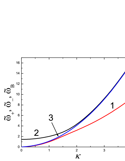
Figure 2: The dispersion law of the elementary excitations with account of pairing correlations: 1) sound branch $\tilde{\omega}_{-}=\omega_{-}/u$; 2) branch with an energy gap $\tilde{\omega}_{+}=\omega_{+}/u$ 3) the Bogolyubov dispersion law $\tilde{\omega}_{B}=\omega_{B}/u$, $\kappa=k/\sqrt{2mU(0)}$. The calculation is performed for $nv=0.1$.

VI Conclusion

We have obtained the system of differential equations (19) – (21) which describes the dynamics of the Bose-Einstein condensate with account of pair correlations. The spectrum of small oscillations in a spatially homogeneous system was studied. It was shown that there are two branches of elementary excitations: one branch with the sound dispersion law in the long wavelength limit and the second branch which has in this limit an energy gap.

It should be noted that the question of the possible existence in the Bose systems of excitations with an energy gap has a long history and has been discussed in many papers (see for e.g. Bijl40 –YuM02 ). The possible existence, in addition to the phonon branch of the spectrum, of the other branch with an energy gap was discussed at a qualitative level in [13, p. 322].

In the experimental paper Rubalko the absorption of microwave radiation was discovered in the superfluid helium at a frequency of about 180 GHz, which authors attributed to the creation of single rotons. However, due to the fact that the momentum of a roton is by orders of magnitude greater than the momentum of a photon at the given frequency, it was suggested in YuM14 that the observed absorption owes its existence to the presence of excitations with energy gap in the superfluid helium. The branches of elementary excitations (one of which is sound and another has an energy gap), which are obtained theoretically in this work, can be considered as a confirmation of the qualitative arguments in favor of the possible existence of the gap excitations in the superfluid helium and the need for modification of the energy spectrum of He-II, which were formulated in YuM14 .

References

• (1) E.P. Gross, Structure of a quantized vortex in boson systems, Il Nuovo Cimento 20, 454-477 (1961).
• (2) L. Pitaevskii, Vortex lines in an imperfect Bose gas, Sov. Phys. JETP. 13, 451-454 (1961).
• (3) L. Pitaevskii, S. Stringari, Bose-Einstein condensation, Oxford University Press, USA, 492 p. (2003).
• (4) C.H. Pethick, H. Smith, Bose-Einstein condensation in dilute gases, Cambridge University Press, 402 p. (2002).
• (5) Yu.M. Poluektov, The polarization properties of an atomic gas in a coherent state, Low Temp. Phys. 37, N12, 986 p. (2011).
• (6) N.N. Bogolyubov, Problems of dynamic theory in statistical physics, in book: Selected works in three volumes, Vol. 2, Naukova Dumka, Kiev, 522 p. (1970).
• (7) N.N. Bogolyubov, Quasiaverages in problems of statistical mechanic, in book: Selected works in three volumes, Vol. 3, Naukova Dumka, Kiev, 488 p. (1971).
• (8) Yu.M. Poluektov, On self-consistent determination of the quasi-average in statistical physics, Low Temp. Phys. 23, N9, 685 p. (1997).
• (9) R.A. Aziz, M.J. Slaman, An examination of ab initio result for the helium potential energy curve, J. Chem. Phys. 94, 8047 p. (1991).
• (10) J.B. Anderson, C.A. Traynor, B.M. Boghosian, An exact quantum Monte Carlo calculation of the helium-helium intermolecular potential, J. Chem. Phys. 99, 345 p. (1993).
• (11) K. A. Brueckner, Theory of nuclear structure. The many body problem. London, Methuen a. o. (1959).
• (12) N.N. Bogolyubov, On the theory of superfluidity, J. Phys. USSR 11, 23-32 (1946); Izv. AN SSSR, Ser. Fiz. 11(1), 77-90 (1947).
• (13) N.N. Bogolyubov and N.N. Bogolyubov, Jr., Introduction to quantum statistical mechanics, Nauka, Moscow, 384 p. (1984). [N.N. Bogolyubov and N.N. Bogolyubov, Jr., Introduction to quantum statistical mechanics, 2nd ed., World Scientific, 440 p.(2009)].
• (14) Yu.M. Poluektov, On the quantum-field description of many-particle Bose systems with spontaneously broken symmetry, Ukr. J. Phys. 52, 578-594 (2007) [arXiv:1306.2103].
• (15) A. Bijl, The lowest wave function of the symmetrical many particles system, Physica 7, 869-886 (1940).
• (16) M. Girardeau, R. Arnowitt, Theory of many-boson system: pair theory, Phys. Rev. 113, 755-761 (1959).
• (17) G. Wentzel, Thermodynamically equivalent Hamiltonian for some many-body problems, Phys. Rev. 120, 1572-1575 (1960).
• (18) M. Luban, Statistical mechanics of a non-ideal boson gas: pair Hamiltonian model, Phys. Rev. 128, 965-987 (1962).
• (19) V.V. Tolmachev, Temperature elementary excitations in a non-ideal Bose-Einstein system (in Russian), DAN SSSR vol.135(4), 825-828 (1960).
• (20) Yu.M. Poluektov, Self-consistent field model for spatially inhomogeneous Bose systems, Low Temp. Phys. 28, N6, 429p. (2002).
• (21) A. Rybalko, S. Rubets, E. Rudavskii, V. Tikhiy, S. Tarapov, R. Golovashchenko, and V. Derkach, Resonance absorption of microwaves in HeII: Evidence for roton emission. Phys. Rev. B. 76, 140503(R) (2007).
• (22) Yu.M. Poluektov, Absorption of electromagnetic field energy by the superfluid system of atoms with a dipole moment, Low Temp. Phys. 40, N5, 389 p. (2014).