Global stability and $H$-theorem in lattice models with non-conservative interactions

Abstract

In kinetic theory, a system is usually described by its one-particle distribution function $f(\bm{r},\bm{v},t)$, such that $f(\bm{r},\bm{v},t)d\bm{r}d\bm{v}$ is the fraction of particles with positions and velocities in the intervals $(\bm{r},\bm{r}+d\bm{r})$ and $(\bm{v},\bm{v}+d\bm{v})$, respectively. Therein, global stability and the possible existence of an associated Lyapunov function or $H$-theorem are open problems when non-conservative interactions are present, as in granular fluids. Here, we address this issue in the framework of a lattice model for granular-like velocity fields. For a quite general driving mechanism, including both boundary and bulk driving, we show that the steady state reached by the system in the long time limit is globally stable. This is done by proving analytically that a certain $H$-functional is non-increasing in the long time limit. Moreover, for a quite general energy injection mechanism, we are able to demonstrate that the proposed $H$-functional is non-increasing for all times. Also, we put forward a proof that clearly illustrates why the “classical” Boltzmann functional $H_{B}[f]=\int\!d\bm{r}\,d\bm{v}f(\bm{r},\bm{v},t)\ln f(\bm{r},\bm{v},t)$ is inadequate for systems with non-conservative interactions. Not only is this done for the simplified kinetic description that holds in the lattice models analysed here but also for a general kinetic equation, like Boltzmann’s or Enskog’s.

I Introduction

In thermodynamics and statistical mechanics, global stability of the equilibrium state is usually proven by introducing a Lyapunov functional Lyapunov (1992). This Lyapunov functional of the probability distribution function (PDF) has the following three properties: (i) it is bounded from below, (ii) it monotonically decreases with time and (iii) its time derivative equals zero only when the PDF is the equilibrium one. Therefore, in the long time limit, the Lyapunov functional must tend to a finite value and thus its time derivative vanishes. As a consequence, any PDF, corresponding to an arbitrary initial preparation, tends to the equilibrium PDF: the equilibrium state is irreversibly approached and said to be globally stable.

The first example of such a Lyapunov functional is the renowned Boltzmann $H$-functional. In the Boltzmann description, the nonequilibrium behaviour of a dilute gas is completely encoded in the one-particle velocity distribution function $f(\bm{r},\bm{v},t)$. By introducing the Stosszahlansatz or Molecular Chaos hypothesis, Boltzmann derived a closed non-linear integro-differential equation for $f(\bm{r},\bm{v},t)$ governing its time evolution Boltzmann (1995). Also, for a spatially homogeneous state, he showed that the functional $H_{B}[f]=\int d\bm{v}f(\bm{v},t)\ln\!f(\bm{v},t)$ has the three properties of a Lyapunov functional. This $H$-theorem shows that all solutions of the Boltzmann equation tend in the long time limit to the Maxwell velocity distribution and irreversibility naturally stems from a molecular picture Lebowitz (1993a, b). Interestingly, a key point for deriving the $H$-theorem is the reversibility of the underlying microscopic dynamics. In an inhomogeneous situation, one has to consider the spatial dependence of the one-particle distribution function $f(\bm{r},\bm{v},t)$, and the above functional must be generalised to

$$H_{B}[f]=\int d\bm{r}\,d\bm{v}f(\bm{r},\bm{v},t)\ln\!f(\bm{r},\bm{v},t).$$ (1)

Provided that the walls of the gas container are smooth, in the sense that there is no energy transport through them, it can be also shown that this is a non-increasing Lyapunov functional Chapman and Cowling (1970).

Another example of a Lyapunov functional can be found in the realm of Markovian stochastic processes. Therein, the stochastic process $X(t)$ is completely determined by the conditional probability density $P_{1|1}(X,t|X_{0},t_{0})$ of finding the system in state $X$ at time $t$, given it was in state $X_{0}$ at time $t_{0}$, and the probability density $P(X,t)$ of finding the system in state $X$ at time $t$ Van Kampen (1992). Both probability densities satisfy the same evolution equation, named the master equation, but with different initial conditions: one always has that $P_{1|1}(X,t_{0}|X_{0},t_{0})=\delta(X-X_{0})$, whereas $P(X,t_{0})=P_{\text{ini}}(X)$, with $P_{\text{ini}}(X)$ corresponding to the (arbitrary) initial preparation. When the stochastic process is irreducible or ergodic, that is, every state can be reached from any other state by a chain of transitions with non-zero probability, there is only one stationary solution of the master equation. In physical systems, this steady solution must correspond to the equilibrium-statistical-mechanics distribution $P_{\text{eq}}(X)$. What is more, a Lyapunov functional can be constructed in the following way,

$$\mathcal{H}[P]=\int dXP_{\text{eq}}(X)\,g\!\left[\frac{P(X,t)}{P_{\text{eq}}(X)}\right],$$ (2)

where $g(x)$ is any positive-definite convex function ($g^{\prime\prime}(x)\geq 0$). It must be stressed that the proof of this $\mathcal{H}$-theorem for master equations rely only on the ergodicity of the underlying microscopic dynamics: it is not necessary to assume that detailed balance, which is connected with the microscopic reversibility, holds Van Kampen (1992).

The most usual choice for $g$ is $g(x)=x\ln x-x+1$, which leads to

$$\mathcal{H}[P]=\int dXP(X,t)\,\ln\!\left[\frac{P(X,t)}{P_{\text{eq}}(X)}\right].$$ (3)

The physical reason behind this choice is the “extensiveness” of $\mathcal{H}[P]$: if the system at hand comprises two independent subsystems $A$ and $B$, so that $dX\equiv dX_{A}dX_{B}$ and $P(X)=P_{A}(X_{A})P_{B}(X_{B})$, one has that $\mathcal{H}[P]=\mathcal{H}_{A}[P_{A}]+\mathcal{H}_{B}[P_{B}]$. It is to consider $-\mathcal{H}$ as a nonequilibrium entropy $S$ that this extensiveness is desirable: in this way, the non-increasing behaviour of $\mathcal{H}$ leads to a non-decreasing time evolution of $S$. Moreover, $H[P]$ remains invariant upon a change of variables $Y=f(X)$, as emphasised in Refs. Marconi et al. (2013); García de Soria et al. (2015).

Although the Boltzmann equation is not a master equation, we may wonder why the expressions for $H_{B}$ in Eq. (1) and $\mathcal{H}[P]$ in Eq. (3) are different. Specifically, we may wonder why not writing

$$H[f]=\int d\bm{r}\,d\bm{v}f(\bm{r},\bm{v},t)\ln\!\left[\frac{f(\bm{r},\bm{v},t)}{f_{\text{eq}}(\bm{v})}\right]$$ (4)

instead of $H_{B}[f]$. Up to now, we have been implicitly considering the “classic” problem with elastic collisions between particles, in which the system eventually reaches thermodynamic equilibrium. Therein, the answer is trivial: since $\ln f_{\text{eq}}(\bm{v})$ is a sum of constants of motion, $H[f]-H_{B}[f]$ is constant and both are utterly equivalent.

Whether there exists an extensive $H$-functional or not is an important question in nonequilibrium statistical physics. If the answer were positive, it would make it possible to define a non-equilibrium entropy $-H$ that monotonically grows for all times, extending the Clausius inequality. In general, the system at hand does not reach equilibrium but a nonequilibrium steady state. Thus, the equilibrium distribution $f_{\text{eq}}$ in $H$ has to be substituted with the stationary one $f_{\text{st}}$. In this context, the field of granular fluids is a benchmark for intrinsically out-of-equilibrium, dissipative, systems: the microscopic dynamics is not time-reversible because collisions between particles are inelastic, but a nonequilibrium steady state can be attained if some driving mechanism injects energy into the system.

In granular fluids, the functionals $H[f]$ and $H_{B}[f]$ are no longer equivalent, since $\ln f_{\text{st}}$ is not a sum of constants of motion. Indeed, for granular gases described by the inelastic Boltzmann equation Pöschel and Luding (2001); Villani (2006), there are some results that hint at $H_{B}$ not being a Lyapunov functional. Within the first Sonine approximation, it has been proven that the time derivative of $H_{B}$ does not have a definite sign in the linear approximation around the steady state Bena et al. (2006). Moreover, Marconi et al. have numerically shown that $H_{B}$ is non-monotonic and even steadily increases from certain initial conditions Marconi et al. (2013). They have also put forward some numerical evidence (further reinforced by García de Soria et al. García de Soria et al. (2015)) in favour of $H$ being a “good” Lyapunov functional. Notwithstanding, only spatially homogeneous situations, in which the $\bm{r}$-dependence of $f$ and thus the integration over $\bm{r}$ may be dropped, have been analysed in Refs. Marconi et al. (2013); García de Soria et al. (2015).

Some years ago, a simplified model for a granular-like velocity field was introduced to study correlations in granular gases Baldassarri et al. (2002). Very recently, a variant of this model on a one-dimensional lattice has been proposed to mimic the velocity component along the shear direction Lasanta et al. (2015), and both its hydrodynamic limit and finite size effects have been analysed Lasanta et al. (2015); Manacorda et al. (2016); Plata et al. (2016). This model has been shown to retain a relevant part of the granular phenomenology: the shear instability of the homogeneous cooling state, the existence of boundary driven steady states such as the Couette and Uniform Shear Flow (USF) states, the renormalisation of the cooling rate due to fluctuations close to the shear instability, etc. Other properties thereof, when it is driven by a mechanism resembling collisions with a randomly moving inelastic wall, have been studied in Ref. Prasad et al. (2017). At the $N$-particle level, the dynamics of the system is governed by a master equation, which is analogous to the Kac equation Kac (1956), that leads to a “kinetic” equation at the one-particle level, which is analogous to the Boltzmann equation. In the latter, the collision term, although being simpler than that in the Boltzmann equation, remains a non-linear integro-differential one Manacorda et al. (2016).

It must be recalled that an analytical proof of either global stability or the $H$-theorem is currently unavailable at the level of the kinetic description for granular gases. This is true even for simple collision terms, such as those corresponding to hard-spheres or the cruder Maxwell particle model (where the collision rate is considered to be velocity-independent), which are considered in the pioneering work in Refs. Marconi et al. (2013); García de Soria et al. (2015). Therefore, it seems worth investigating this subject in simplified models, for which analytical calculations are more feasible.

Our main goal here is to investigate the global stability and the possibly associated $H$-theorem in the above class of lattice models. Unlike the approach in Refs. Marconi et al. (2013); García de Soria et al. (2015), we do not restrict ourselves to spatially homogeneous situations but consider the whole space and velocity dependence of the one-particle PDF $f(\bm{r},\bm{v},t)$. Specifically, we introduce a general energy injection mechanism, in which the system may be driven both through the boundaries and in the bulk. We show that, under quite general conditions, the steady state is globally stable: independently of the initial preparation, the system always ends up in the steady state. Interestingly, it is not necessary to have an $H$-theorem to prove this: it suffices to show that $H$ is decreasing in the long time limit, not for all times. In this sense, the situation is analogous to the proof of the tendency towards the equilibrium curve in systems whose dynamics is governed by master equations with time-dependent transition rates Brey and Prados (1993, 1994); Brey et al. (1994); Vlad and Ross (1997); Vlad et al. (1998); Prados et al. (2000); Earnshaw and Keener (2010).

Our proof of global stability also enables us to show the inadequacy of Boltzmann’s $H_{B}$ as a candidate for Lyapunov functional in inelastic systems. Not only is this done for the simplified models considered in the paper, but for a general collision term that does not conserve energy in collisions. Therefore, this result also applies to the inelastic Boltzmann or Enskog equations used in granular fluids. The main idea is that the sign of $dH_{B}/dt$ can be reversed by a suitable choice of the initial PDF, and thus cannot have a definite sign. In this respect, our result generalises that in Ref. Bena et al. (2006), which was derived within the first Sonine approximation of the inelastic Boltzmann equation, to an arbitrary collision kernel with non-conservative interactions.

Having proved global stability by showing that $H$ is a non-increasing functional for long times, a natural question remains. Is it $H$ a Lyapunov function, that is, a non-increasing functional for all times? There does not seem to be a unique proof, valid for any driving mechanism, even within our simplified model. Nevertheless, we have been able to derive a specific proof for a quite general driving mechanism, which includes as limiting cases both the sheared system, in which the steady state is the USF state, and the uniformly heated system by means of the so-called stochastic thermostat Van Noije and Ernst (1998); Montanero and Santos (2000); García de Soria et al. (2009); García de Soria et al. (2012); Pagonabarraga et al. (2002); Maynar et al. (2009); Prados and Trizac (2014); Trizac and Prados (2014); Prasad et al. (2013). The proof is based on a suitable expansion of the one-particle PDF in Hermite polynomials, which is a generalisation of the usual Sonine expansion of kinetic theory.

The paper is organised as follows. In Sec. II, we briefly introduce the model, its dynamics and the continuum limit. Section III is devoted to the proof of the global stability of the nonequilibrium steady states, for a general energy injection mechanism. The inadequacy of Boltzmann’s $H_{B}$ as a Lyapunov functional for inelastic systems is discussed in Sec. IV. Later, in Sec. V, we consider some concrete physical situations in our model, which include the sheared and the uniformly heated systems. Therein, we show that $H[f]$ is a monotonically decreasing Lyapunov functional. Finally, Sec. VI gives the main conclusions of the paper. Some technical details, which are omitted in the main text, are given in the Appendices.

II The model: dynamics and continuum limit

Here, we present the general class of models that was introduced in Ref. Lasanta et al. (2015), focusing on the continuum description obtained in the large system size limit Manacorda et al. (2016). Specifically, our system is defined on a $1$d lattice: at each lattice site $l$, there is a particle with velocity $v_{l}$. Thus, at a given time $\tau$, the configuration of the system is completely determined by $\bm{v}\equiv\{v_{1},...,v_{N}\}$. The dynamics proceeds through inelastic nearest-neighbour binary collisions: each pair $(l,l+1)$ collides inelastically with a characteristic rate $\omega^{-1}$, independently of their relative velocity (the so-called Maxwell-molecule model Ben-Naim and Krapivsky (2003)) and the state of the other pairs. We introduce the operator $\hat{b}_{l}$ that transforms the pre-collisional velocities into the post-collisional ones,

$$\hat{b}_{l}v_{l} =v_{l}-\frac{1+\alpha}{2}\left(v_{l}-v_{l+1}\right),$$ (5a)

$$\hat{b}_{l}v_{l+1} =v_{l+1}+\frac{1+\alpha}{2}\left(v_{l}-v_{l+1}\right),$$ (5b)

where $\alpha$ is the normal restitution coefficient, with $0<\alpha\leq 1$.

In addition to collisions, the system is heated by a stochastic force that is modelled by a white noise, the so-called stochastic thermostat Van Noije and Ernst (1998); Montanero and Santos (2000); García de Soria et al. (2009); García de Soria et al. (2012); Pagonabarraga et al. (2002); Maynar et al. (2009); Prados and Trizac (2014); Trizac and Prados (2014); Prasad et al. (2013). Specifically, for a short time interval, the change of the velocity due to the heating is given by

$$\left.\Delta v_{i}(\tau)\right|_{\text{noise}} \equiv \left.v_{i}(\tau+\Delta\tau)-v_{i}(\tau)\right|_{\text{noise}}$$ (6)

$$= \left(\xi_{i}(\tau)-\frac{1}{N}\sum_{j=1}^{N}\xi_{j}(\tau)\right)\Delta\tau,$$

where $\xi_{i}(t)$ are Gaussian white noises, verifying

$$\langle\xi_{i}(\tau)\rangle_{\text{noise}}=0,\quad\langle\xi_{i}(\tau)\xi_{j}(\tau^{\prime})\rangle_{\text{noise}}=\chi\delta_{ij}\delta(\tau-\tau^{\prime}),$$ (7)

for $i,j=1,\ldots,N$. Above, $\chi$ is the amplitude of the noise, and $\langle\cdots\rangle_{\text{noise}}$ denotes the average over the different realisations of the noise. Note that this version of the stochastic thermostat conserves total momentum, a necessary condition to have a steady state Maynar et al. (2009); Prasad et al. (2013).

We define $P_{N}(\bm{v},\tau)$ as the probability density of finding the system in state $\bm{v}$ at time $\tau$. The stochastic process $\bm{v}(\tau)$ is Markovian and the equation governing the time evolution of $P_{N}(\bm{v},\tau)$ has two contributions. First, we have a master equation contribution stemming from collisions Manacorda et al. (2016); Plata et al. (2016)

$$\left.\partial_{\tau}P_{N}(\bm{v},\tau)\right|_{\text{coll}}=\omega\sum_{l=1}^{N}\left[\frac{P_{N}(\hat{b}_{l}^{-1}\bm{v},\tau)}{\alpha}-P_{N}(\bm{v},\tau)\right],$$ (8)

in which the operator $\hat{b}_{l}^{-1}$ is the inverse of $\hat{b}_{l}$, that is, it changes the post-collisional velocities into the pre-collisional ones when the colliding pair is $(l,l+1)$. Second, there is a Fokker-Planck contribution stemming from the stochastic forcing Marconi et al. (2013); García de Soria et al. (2015)

$$\left.\partial_{\tau}P_{N}(\bm{v},\tau)\right|_{\text{noise}}=\frac{\chi}{2}\sum_{i,j=1}^{N}\left(\delta_{ij}-\frac{1}{N}\right)\frac{\partial^{2}}{\partial v_{i}\partial v_{j}}P_{N}(\bm{v},\tau).$$ (9)

The time evolution of $P_{N}(\bm{v},\tau)$ is obtained by combining Eqs. (8) and (9), that is,

$$\partial_{\tau}P_{N}(\bm{v},\tau)=\left.\partial_{\tau}P_{N}(\bm{v},\tau)\right|_{\text{coll}}+\left.\partial_{\tau}P_{N}(\bm{v},\tau)\right|_{\text{noise}}.$$ (10)

In this work, we focus on the evolution of quantities that can be written in terms of the one-particle distribution function, namely

$$P_{1}(v;l,\tau)=\int d\bm{v}P_{N}(\bm{v},\tau)\delta(v_{l}-v).$$ (11)

All the one-site velocity moments can be calculated from $P_{1}$,

$$\langle v_{l}^{n}(\tau)\rangle\equiv\int_{-\infty}^{+\infty}dv\,v^{n}P_{1}(v;l,\tau).$$ (12)

The first two moments give the hydrodynamic fields: the average velocity $u_{l}(\tau)$ and granular temperature $T_{l}(\tau)$ , which are defined by the relations

$$u_{l}(\tau)\equiv\langle v_{l}\rangle,\qquad T_{l}(\tau)\equiv\langle v_{l}^{2}(\tau)\rangle-u_{l}^{2}(\tau).$$ (13)

Here, we do not write the evolution equations on the lattice for either $P_{1}$ or the hydrodynamic fields ($u$ and $T$), since they are not necessary for our present purposes. The unforced case ($\chi=0$) can be found in Ref. Manacorda et al. (2016). However, we would like to stress that the evolution equation for $P_{1}$ is not closed, since the collision term involves the two-particle distribution function $P_{2}(v,v^{\prime};l,l+1,\tau)$. As usual in kinetic theory, one can write a closed equation for $P_{1}$ after introducing the Molecular Chaos assumption, that is, $P_{2}(v,v^{\prime};l,l+1,\tau)=P_{1}(v;l,\tau)P_{1}(v^{\prime};l+1,\tau)+O(N^{-1})$. In other words, one assumes that the correlations at different sites are of the order of $N^{-1}$ and thus negligible in the large system size limit.

The continuum limit of the model is introduced for large system size $N\gg 1$, in which we expect the average velocity $u_{l}$ and temperature $T_{l}$ to be smooth functions of space and time. This is expressed mathematically by defining “hydrodynamic” continuous space and time variables by $x=l/N$ and $t=\omega\tau/N^{2}$, respectively Manacorda et al. (2016). Note that $0\leq x\leq 1$ and $t\geq 0$. In the continuum limit, the one-particle distribution function also becomes a smooth function of $x$ and $\tau$, $P_{1}(v;x,t)\equiv P_{1}(v;l=Nx,\tau=N^{2}t/\omega)$.

From now on, we use the usual notation in kinetic theory $f(x,v,t)\equiv P_{1}(v;x,t)$. The physical picture is straightforward: $f(x,v,t)dxdv$ gives the fraction of the total number of particles with positions between $x$ and $x+dx$ and velocities between $v$ and $v+dv$. We have that $\int_{-\infty}^{+\infty}dv\,f(x,v,t)=1$ for all $x$ and $t$, since there is no mass transport in the system. The time evolution of $f$ is governed by the non-linear integro-differential (pseudo-Boltzmann) equation Manacorda et al. (2016)

$$\partial_{t}f=\partial_{x}^{2}f+\frac{\nu}{2}\partial_{v}\left\{[v-u(x,t)]f\right\}+\frac{\xi}{2}\partial_{v}^{2}f,$$ (14)

where $u(x,t)$ is the local average velocity, $\nu$ is the macroscopic dissipation coefficient and $\xi$ is the macroscopic noise strength, which are respectively given by

$$\nu=(1-\alpha^{2})N^{2},\qquad\xi=\frac{\chi N^{2}}{\omega}.$$ (15)

This shows that the microscopic noise strength $\chi$ must scale as $N^{-2}$ in order to have a finite contribution in the continuum limit. Of course, for $\xi=0$, we recover the kinetic equation for the case in which there is no stochastic forcing, see Ref. Manacorda et al. (2016). The $N$-scaling of the macroscopic dissipation coefficient $\nu$ is similar to that found in the dissipative version of the Kipnis-Marchioro-Presutti model Kipnis et al. (1982); Prados et al. (2011, 2012); Hurtado et al. (2013); Lasanta et al. (2016).

The average velocity $u(x,t)$ and granular temperature $T(x,t)$ are the continuum limit of $u_{l}$ and $T_{l}$ defined in Eq. (13),

$$u(x,t)\equiv\langle v\rangle(x,t),\qquad T(x,t)\equiv\langle v^{2}\rangle(x,t)-u^{2}(x,t),$$ (16)

where the velocity moments are given by $\langle v^{n}\rangle(x,t)=\int dv\,v^{n}f(x,v,t)$. From the kinetic equation for $f(x,v,t)$, one can derive the evolution equations of $u$ and $T$,

$$\partial_{t}u =\partial_{xx}u,$$ (17a)

$$\partial_{t}T =-\nu T+\partial_{x}^{2}T+2\left(\partial_{x}u\right)^{2}+\xi.$$ (17b)

On the one hand, Eq. (17a) is a diffusion equation for the average velocity, which expresses the conservation of total momentum. On the other hand, the temperature equation (17b) contains a purely dissipative term $-\nu T$ that stems from the inelasticity of collisions and always contributes to “cooling” the system, a diffusive term $\partial_{x}^{2}T$, a viscous heating term $2\left(\partial_{x}u\right)^{2}$, and finally the term corresponding to the uniform heating $\xi$. Of course, either the kinetic equation for $f$ or the average equations for $(u,T)$ must be complemented with suitable boundary conditions in each physical situation.

II.1 Non-equilibrium steady states and boundary conditions

We are interested in driven cases, in which there is an input of energy that balances (in average) the energy loss in collisions, so that the system eventually reaches a steady state. These non-equilibrium steady states (NESS) are described by the corresponding stationary solutions $f_{\text{st}}(x,v)$ of the kinetic equation, which verify

$$0=\partial_{x}^{2}f_{\text{st}}+\frac{\nu}{2}\partial_{v}\left\{[v-u_{\text{st}}(x)]f_{\text{st}}\right\}+\frac{\xi}{2}\partial_{v}^{2}f_{\text{st}}.$$ (18)

where $u_{\text{st}}(x)=\int dv\,vf_{\text{st}}(x,v)$ is the stationary average velocity profile. To be concrete, we consider two cases: a system that is (a) sheared and (b) uniformly heated.

First, let us consider a sheared system: there is no stochastic forcing, $\xi=0$, and the driving is introduced by imposing a velocity difference (“shear”) between the left and right edges of the system. At the level of the hydrodynamic description, the corresponding boundary conditions are

$$u(1,t) =u(0,t)+a, u^{\prime}(1,t) =u^{\prime}(0,t),$$ (19a)

$$T(1,t) =T(0,t), T^{\prime}(1,t) =T^{\prime}(0,t),$$ (19b)

which are said to be of Lees-Edwards type Lees and Edwards (1972). We have used ^′ to denote spatial derivative. The imposed shear allows the viscous heating term, which is proportional to $(\partial_{x}u)^{2}$, to compensate for the energy dissipation term, $-\nu T$. The boundary conditions for the one-particle distribution function read

$$f(1,v,t)=f(0,v-a,t),\quad f^{\prime}(1,v,t)=f^{\prime}(0,v-a,t),$$ (20a)

from which Eq. (19) directly follow. Equation (20) has a simple physical interpretation: particles that leave the system through its right edge with velocity $v$ are reinserted through its left edge with velocity $v-a$.

The steady state for the sheared system is known as the USF state, which has a linear velocity profile and a homogeneous temperature,

$$u_{\text{st}}(x)=a\left(x-\frac{1}{2}\right),\quad T_{\text{st}}=\frac{2a^{2}}{\nu}.$$ (21)

For our simplified model, the stationary PDF is Gaussian,

$$f_{\text{st}}(x,v)=\left(2\pi T_{\text{st}}\right)^{-1/2}\exp\left[-\frac{(v-u_{\text{st}}(x))^{2}}{2T_{\text{st}}}\right].$$ (22)

An extensive investigation of the sheared system, at the level of the average hydrodynamic equations, can be found in Ref. Manacorda et al. (2016).

Second, we address the uniformly heated system, in which there is no shear, $a=0$, but there is stochastic forcing, $\xi\neq 0$. In this case, we have the usual periodic boundary conditions. In particular, for the PDF we have

$$f(1,v,t)=f(0,v,t),\quad f^{\prime}(1,v,t)=f^{\prime}(0,v,t).$$ (23)

In the steady state, the system is homogeneous: there is no average velocity and the temperature is uniform,

$$u_{\text{st}}(x)=0,\quad T_{\text{st}}=\frac{\xi}{\nu}.$$ (24)

The corresponding stationary PDF is also Gaussian,

$$f_{\text{st}}(\cancel{x},v)=\left(2\pi T_{\text{st}}\right)^{-1/2}\exp\left[-\frac{v^{2}}{2T_{\text{st}}}\right].$$ (25)

With this “stochastic thermostat” forcing, the system remains homogeneous for all times if it is initially so, as is also the case of a inelastic gas of hard particles described by the inelastic Boltzmann equation Van Noije and Ernst (1998).

III Global stability

In this section, we analyse the global stability of the nonequilibrium stationary solutions of the kinetic equation (14) submitted to quite a general class of boundary conditions. Following the discussion in the introduction, we define the $H$-functional as

$$H[f]=\int\!\!dx\,dvf(x,v,t)\ln\!\left[\frac{f(x,v,t)}{f_{\text{st}}(x,v)}\right].$$ (26)

Let us consider the time evolution of $H[f]$. It is directly obtained that

$$\frac{dH}{dt}=\int\!\!dx\,dv\,\partial_{t}{f}\ln\left(\frac{f}{f_{\text{st}}}\right)=\int\!\!dx\,dv\,\mathcal{L}f\,\ln\left(\frac{f}{f_{\text{st}}}\right),$$ (27)

where $\mathcal{L}$ stands for the nonlinear evolution operator on the rhs of the kinetic equation (14), that is, $\partial_{t}{f}=\mathcal{L}f$. Now we note the following property: if we define $\Delta f=f-f_{\text{st}}$ to be the deviation of the PDF from the steady state, the linear terms in the deviation vanishes, since both factors in the integrand of (27) are equal to zero for $f=f_{\text{st}}$. This is a desirable property: were it not true, the sign of $dH/dt$ could be reversed for initial conditions close enough to the steady state by simply reversing the initial value of $\Delta f$. Thus, the existence of an $H$-theorem would be utterly impossible, see also next Section.

Then, we can write

$$\frac{dH}{dt}=\int\!\!dx\,dv\,\mathcal{L}f\,\ln\left(\frac{f}{f_{\text{st}}}\right)-\int\!\!dx\,dv\,\mathcal{L}f_{\text{st}}\,\frac{f-f_{\text{st}}}{f_{\text{st}}}.$$ (28)

Now, the idea is to split the operator $\mathcal{L}$ into the three contributions on the rhs of Eq. (14): first, the diffusive one; second, the one proportional to $\nu$, which is intrinsically dissipative; and third, the one proportional to the noise strength $\xi$: $\mathcal{L}_{\text{diff}}$, $\mathcal{L}_{\text{inel}}$ and $\mathcal{L}_{\text{noise}}$, respectively. Accordingly, we have that the time derivative of $H$ has three contributions,

$$\frac{dH}{dt}=\left.\frac{dH}{dt}\right|_{\text{diff}}+\left.\frac{dH}{dt}\right|_{\text{inel}}+\left.\frac{dH}{dt}\right|_{\text{noise}},$$ (29)

obtained by inserting into Eq. (28) the relevant part of the evolution operator $\mathcal{L}$. Note that, although $\mathcal{L}f_{\text{st}}=0$, in general $\mathcal{L}_{\text{diff}}f_{\text{st}}\neq 0$, $\mathcal{L}_{\text{inel}}f_{\text{st}}\neq 0$ and $\mathcal{L}_{\text{noise}}f_{\text{st}}\neq 0$.

After some tedious but easy algebra, a summary of which is given in Appendix A, the following expressions are derived. Firstly, for the diffusive term,

$$\left.\frac{dH}{dt}\right|_{\text{diff}}=-\int\!\!dx\,dv\,f\left(\partial_{x}{\ln f}-\partial_{x}{\ln f_{\text{st}}}\right)^{2}\leq 0.$$ (30)

Secondly, for the inelastic term, proportional to $\nu$,

$$\left.\frac{dH}{dt}\right|_{\text{inel}}=-\frac{\nu}{2}\int\!\!dx\left(u-u_{\text{st}}\right)\int\!\!dvf\,\partial_{v}{\ln f_{\text{st}}}.$$ (31)

Finally, the noise term, proportional to $\xi$, reads

$$\left.\frac{dH}{dt}\right|_{\text{noise}}=-\frac{\xi}{2}\int\!\!dx\,dv\,f\left(\partial_{v}{\ln f}-\partial_{v}{\ln f_{\text{st}}}\right)^{2}\leq 0.$$ (32)

These results, and the following throughout this section, are valid for a quite general set of boundary conditions, leading to the cancellation of all the boundary terms arising after integrating by parts, as detailed in Appendix A. This set includes but is not limited to the Lees-Edwards and periodic boundary conditions corresponding to the sheared and uniformly heated situations, respectively. For instance, they also apply to the Couette state, in which the system is driven by keeping its two edges at two (in general, different) fixed temperatures $T_{L}$ and $T_{R}$.

The inelastic term $dH/dt|_{\text{inel}}$ in Eq. (31) does not have a definite sign in general. Therefore, it is the inelastic term that prevents us from proving $H$ to be a non-increasing function of time. It must be stressed that the diffusive, inelastic and noise contributions to $dH/dt$ in Eqs. (30)-(31) come exclusively from the diffusive, noise and inelastic contributions in the kinetic equation, respectively, only once the linear terms has been subtracted as is done in Eq. (28): see Appendix A for details.

Despite the above discussion, global stability of the steady state can be established without proving an $H$-theorem. The key point is the following: the long time limit of $dH/dt$ is non-positive and thus $H$ has a finite limit, since it is bounded from below. Therefore, $dH/dt$ tends to zero in the long time limit and it can be shown that this is only the case if $f(x,v,\infty)\equiv\lim_{t\to\infty}f(x,v,t)=f_{\text{st}}(x,v)$.

The average velocity $u(x,t)$ satisfies a diffusive equation (17a), and thus it irreversibly tends to the steady profile corresponding to the given boundary conditions in the long time limit. Therefore, $u(x,\infty)\equiv\lim_{t\to\infty}u(x,t)=u_{\text{st}}(x)$ and taking into account Eq. (31),

$$\lim_{t\to\infty}\left.\frac{dH}{dt}\right|_{\text{inel}}=0\Rightarrow\lim_{t\to\infty}\frac{dH}{dt}\leq 0.$$ (33)

Since $H[f]$ is bounded from below, the only possibility is

$$\lim_{t\to\infty}\frac{dH}{dt}=0,$$ (34)

and all the contributions to $dH/dt$ in Eqs. (30)-(32) vanish in the long time limit. The vanishing of Eq. (30) imposes that $f(x,v,\infty)=f_{\text{st}}(x,v)\phi(v)$, where $\phi(v)$ is an arbitrary function of $v$. For $\xi\neq 0$, Eq. (32) implies that $\phi(v)$ must be a constant, independent of $v$, and normalisation yields $\phi(v)=1$. For $\xi=0$, Eq. (32) identically vanishes but it can be also shown that $\phi(v)=1$ by using the kinetic equation in the limit as $t\to\infty$. Therefore, for arbitrary $\xi$, including $\xi=0$, we have that

$$f(x,v,\infty)=f_{\text{st}}(x,v).$$ (35)

This completes the proof. The steady distribution $f_{\text{st}}(x,v)$ is globally stable: each time evolution $f(x,v,t)$ (corresponding to a given initial condition) tends to it in the long time limit.

IV Inadequacy of $H_{B}$ as a Lyapunov functional for non-conservative systems

Here we show that Boltzmann’s $H_{B}[f]$ cannot be used to build a Lyapunov functional for intrinsically dissipative systems, in agreement with the numerical results by Marconi et al. Marconi et al. (2013). Not only do we prove it for the simplified models considered here, but for a general kinetic equation in which energy is not conserved in collisions, such as the inelastic Boltzmann or Enskog equations. To keep the notation simple, we still write $\partial_{t}{f}=\mathcal{L}f$, but now $\mathcal{L}$ stands for the evolution operator in the considered kinetic description, which is nonlinear in general.

First, we restrict ourselves to homogeneous situations and thus drop the integral over $x$,

$$H_{B}[f]= \int\!\!dvf\ln f$$ (36a)

$$\frac{dH_{B}}{dt}= \int\!\!dv\,\partial_{t}{f}\ln f=\int\!\!dv\,\mathcal{L}f\,\ln f,$$ (36b)

Also, we consider a system that is initially close to the steady state, such that we can expand everything in powers of $\Delta f=f-f_{\text{st}}$. Then,

$$\mathcal{L}f\equiv\mathcal{L}(f_{\text{st}}+\Delta f)=\cancelto{0}{\mathcal{L}f_{\text{st}}}+\mathcal{L}_{\text{lin}}\Delta f+O(\Delta f)^{2},$$ (37)

in which $\mathcal{L}_{\text{lin}}$ is the linearised evolution operator. Neglecting $O(\Delta f)^{2}$ terms, the linear approximation arises,

$$\left.\frac{dH_{B}}{dt}\right|_{\text{lin}}=\int\!\!dv\,(\mathcal{L}_{\text{lin}}\Delta f)\,\ln f_{\text{st}}=\left.\frac{d}{dt}\langle\ln f_{\text{st}}\rangle\right|_{\text{lin}}.$$ (38)

On the one hand, the linear contribution vanishes in the elastic case: $\ln f_{\text{st}}$ is a sum of constants of motion, which are unchanged by the linearised kinetic operator. Then, $H_{B}$ can be a candidate for a Lyapunov functional. On the other hand, only mass and linear momentum are conserved for non-conservative interactions. Thus, no longer is $\ln f_{\text{st}}$ a sum of conserved quantities, and

$$\left.\frac{dH_{B}}{dt}\right|_{\text{lin}}\neq 0.$$ (39)

Therefore, by changing the initial sign of $\Delta f=f-f_{\text{st}}$, which can always be done, the initial sign of $dH_{B}/dt$ is reversed and $H_{B}$ cannot be a Lyapunov functional.

In Fig. 1, we show the evolution of $H_{B}$ in our kinetic model. We consider a uniformly heated system, so that the system remain homogeneous for all times, as described in Sec. II.1. Two different initial conditions are considered, corresponding to Gaussian distributions with zero average velocity but non-steady values of the temperature, specifically $1.1\,T_{\text{st}}$ and $0.9\,T_{\text{st}}$. We can see how, in agreement with our discussion, not only is one of the functionals increasing, but also it can be obtained as the mirror image of the decreasing one through the stationary value. Technical details about the simulation are provided in Appendix B.

Taking into account the specific (Gaussian) shape of the steady PDF for the uniformly heated system, as given by Eq. (25), the time derivative of $H_{B}$ in Eq. (38) reduces to

$$\frac{dH_{B}}{dt}=-\frac{1}{2T_{\text{st}}}\frac{d\langle v^{2}\rangle}{dt}.$$ (40)

Since the plots in Fig. 1 correspond to evolutions of the system for which $u(x,t)\equiv 0$ for all times, therein $\langle v^{2}\rangle=T$ and, consistently, the $H_{B}$-curve corresponding to an initial value of the temperature that is higher (lower) than the steady one monotonically increases (decreases).

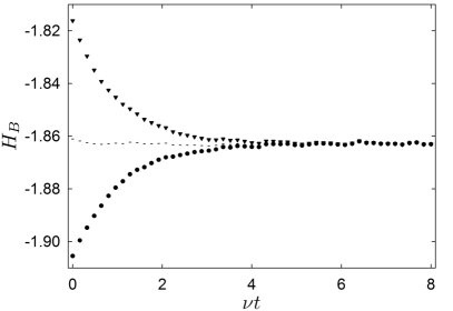
Figure 1: Evolution of the functional $H_{B}$ for two different initial conditions in a uniformly heated system. Both simulations start from the stationary Gaussian shape but with a homogeneous temperature slightly shifted from the stationary one: (i) $T(t=0)=1.1\,T_{\text{st}}$ (circles) and (ii) $T(t=0)=0.9\,T_{\text{st}}$ (triangles). As predicted by the linear approximation, both functionals are symmetric with respect to the stationary value, which is schematically illustrated by plotting their mean value (dashed line). A system with $N=330$ sites has been considered, with $\nu=20$ and $\xi=50$. The plots correspond to averages over $3000$ trajectories.

This is consistent with the situation found in Ref. Bena et al. (2006), in which the uniformly heated granular gas described by the inelastic Boltzmann equation was investigated within the first Sonine approximation. Therein, the entropy production was shown to have linear terms in the deviations of the temperature and the excess kurtosis. Also, our result is consistent with the numerical results in Ref. Marconi et al. (2013) for several collision models. The above argument also proves why $H_{B}$ is not non-increasing for an elastic system immersed in a heat bath at a temperature different from the initial temperature of the gas, as also observed in Ref. Marconi et al. (2013). Although $\ln f_{\text{st}}$ is conserved in collisions, the evolution operator includes a term coming from the interaction with the bath that does not conserve the kinetic energy, and again $dH/dt|_{\text{lin}}\neq 0$, making it impossible for $H_{B}$ to be a Lyapunov functional.

In spatially non-homogeneous situations, the main difference is that an additional integral over $x$ is present, both in $H_{B}$ and, consequently, $dH_{B}/dt$. There is no reason to expect this integral over space to make $dH/dt|_{\text{lin}}$ vanish, since one still has that

$$\left.\frac{dH_{B}}{dt}\right|_{\text{lin}}=\left.\frac{d}{dt}\langle\ln f_{\text{st}}\rangle\right|_{\text{lin}},$$ (41)

and, in general, $\ln f_{\text{st}}$ is not a sum of constants of motion. In fact, again the sign of $\left.dH_{B}/dt\right|_{\text{lin}}$ is reversed when $\Delta f\to-\Delta f$, similarly to the homogeneous case. We have numerically checked this prediction for the sheared system, with the resulting evolution of $H_{B}$ being completely similar to that for the uniformly heated case in Fig. 1, and thus is not shown here.

V $H$-theorem for some specific NESS

Here we prove that the functional $H[f]$ is monotonically decreasing for all times in some specific physical situations. Our proof applies both to the sheared and uniformly heated systems described in Sec. II.1. To be as general as possible, we consider a system that is both heated and sheared: $a\neq 0$ and $\xi\neq 0$. In this situation, the boundary conditions for the PDF are given by Eq. (20), which lead to Eqs. (19a) and (19b) for the averages $u(x,t)$ and $T(x,t)$.

The steady solution of the hydrodynamic equations is

$$u_{\text{st}}(x)=a\left(x-\frac{1}{2}\right),\qquad T_{\text{st}}=\frac{2a^{2}+\xi}{\nu}.$$ (42)

On the one hand, the average velocity has a linear profile, similarly to the situation in the USF state. On the other hand, the temperature remains homogeneous but its steady value has two contributions, one coming from the shear and the other from the stochastic thermostat. The viscous heating $2(\partial_{x}{u})^{2}$ and uniform heating $\xi$ terms cancel the cooling term $-\nu T$ for all $x$. The stationary solution of the kinetic equation is readily found:

$$f_{\text{st}}(x,v)=(2\pi T_{\text{st}})^{-1/2}\exp\left[-\frac{\left(v-u_{\text{st}}(x)\right)^{2}}{2T_{\text{st}}}\right],$$ (43)

that is, the Gaussian distribution corresponding to the hydrodynamic fields in Eq. (42). Of course, the USF state and NESS of the uniformly heated system in Sec. II.1 can be easily recovered as particular cases of Eq. (43): for $(a\neq 0,\xi=0)$ and $(a=0,\xi>0$), respectively.

Then, we turn now to the question of the existence of an $H$-theorem, that is, the existence of a nonequilibrium entropy ensuring the monotonic approach of the one-particle PDF to the steady state. Our starting point is the following expansion of the one-particle PDF in Hermite polynomials,

$$f(x,v,t)= \frac{1}{\sqrt{2\pi T(x,t)}}\exp\left[-\frac{[v-u(x,t)]^{2}}{2T(x,t)}\right]$$

$$\times\left[1+\sum_{n=3}^{\infty}\gamma_{n}(x,t)\,H_{n}\!\!\left(\frac{v-u(x,t)}{\sqrt{T(x,t)}}\right)\right],$$ (44)

which is known as the Gram-Charlier series Chebyshev (1890); Charlier (5 06); Edgeworth (1905); Wallace (1958). Therein, $u(x,t)$ and $T(x,t)$ are the (exact) average velocity and temperature stemming from the hydrodynamic equations for the considered distribution. The above expansion is suggested by the Gaussian shape of the stationary PDF in Eq. (43). Now we define

$$c=\frac{v-u(x,t)}{\sqrt{T(x,t)}},\quad\tilde{f}(x,c,t)=\sqrt{T(x,t)}\,f(x,v,t),$$ (45)

From the orthogonality relation of the Hermite polynomials Abramowitz and Stegun (1972), it is readily obtained that

$$\gamma_{n}(x,t)=\frac{1}{n!}\int\!\!dc\,H_{n}(c)\tilde{f}(x,c,t).$$ (46)

Also, we could write $\gamma_{n}$ as a combination of moments of the distribution.

Some comments on the Gram-Charlier expansion are pertinent. First, note that $n\geq 3$ in the sum: $\gamma_{1}=\gamma_{2}=0$ because the zero-th order Gaussian contribution exactly gives the first two moments $u(x,t)$ and $\langle v^{2}\rangle(x,t)=u^{2}(x,t)+T(x,t)$. Second, if $f(x,v,t)$ were symmetric with respect to $v=u$, that is, $\langle(v-u)^{2n+1}\rangle=0$ for all $n\in\mathbb{N}$, only even values of $n$ would be present in the sum and one would end up with the usual expansion in Sonine-Laguerre polynomials of kinetic theory. Finally, it is worth stressing that the series (44) converges for functions such that the tails of $\tilde{f}(x,c,t)$ approach zero faster than $e^{-c^{2}/4}$ for $c\to\pm\infty$ Cramér (1925); Szegö (1939); Wallace (1958).

After a lengthy but straightforward calculation, which is summarised in Appendix C, it is shown that

$$\frac{dH}{dt}=A(t)+B(t),\quad\text{with both }A(t),B(t)\leq 0.$$ (47)

The expressions for $A(t)$ and $B(t)$ are

$$A(t)=-\int\!\!dx\,T\left[\left(\frac{u^{\prime}}{T}-\frac{u_{\text{st}}^{\prime}}{T_{\text{st}}}\right)^{2}+\frac{\xi}{2}\left(\frac{1}{T}-\frac{1}{T_{\text{st}}}\right)^{2}\right]$$ (48)

and

$$B(t)= -\frac{1}{\sqrt{2\pi}}\int\!\!dx\,dc\,\frac{e^{-c^{2}/2}}{1+\sum_{n=3}^{\infty}\gamma_{n}H_{n}(c)}\left\{\frac{T^{\prime}}{2T}H_{2}(c)+\sum_{n=3}^{\infty}\gamma_{n}^{\prime}H_{n}(c)-\sum_{n=3}^{\infty}\frac{\gamma_{n}u^{\prime}}{\sqrt{T}}nH_{n-1}(c)\right.$$

$$\left.+\sum_{n=3}^{\infty}\frac{\gamma_{n}T^{\prime}}{2T}\left[H_{n+2}(c)+nH_{n}(c)\right]\right\}^{2}-\frac{\xi}{2\sqrt{2\pi}}\int\!\!dx\,dc\,\frac{e^{-c^{2}/2}}{1+\sum_{n=3}^{\infty}\gamma_{n}H_{n}(c)}\frac{1}{T}\left[\sum_{n=3}^{\infty}\gamma_{n}nH_{n-1}(c)\right]^{2}.$$ (49)

We recall that the prime denotes spatial derivative.

Therefore, $dH/dt\leq 0$ for all times and we have shown that the $H$-theorem holds for the sheared and heated system. Rigorously, our proof holds for those PDFs such that the above Hermite expansion converges. Note that the proof remains valid for the approach to any NESS, whose PDF is a Gaussian with a homogeneous temperature, independently of the corresponding boundary conditions. In Sec. III, we have already demonstrated that $dH/dt$ only vanishes for $f(x,v,\infty)=f_{\text{st}}(x,v)$, but the same result can be rederived here in a different way. By imposing that both $A(t)$ and $B(t)$ vanish in the long time limit and making use of the hydrodynamic equations for the averages, it can be shown that $u(x,\infty)=u_{\text{st}}(x)$, $T(x,\infty)=T_{\text{st}}$ and $\gamma_{n}(x,\infty)=0$, $\forall n\geq 3$.

V.1 Numerical results for the USF state

Here we consider the sheared system, and we numerically check our theoretical predictions. Throughout this section, we use the values of the parameters $\nu=20$, $a=5$ and $\xi=0$ (there is no stochastic forcing).

Firstly, in Figure 2, we show the evolution of the distribution and the $H$-functional from a Gaussian initial condition with the steady velocity profile $u(x,0)=u_{\text{st}}(x)$ but a higher temperature, $T(t=0)=7\,T_{\text{st}}$. In panel (a), we depict the velocity distribution at $x=1/4$ for several times. All of them are Gaussian, which agrees with the theoretical prediction of the kinetic equation: when the initial velocity profile coincides with the steady one and only the temperature is perturbed, an initially Gaussian PDF remains Gaussian for all times. Indeed, we can see in the inset how the excess kurtosis $\kappa=\langle[v-u(x)]^{4}\rangle/\langle[v-u(x)]^{2}\rangle^{2}-3$ only fluctuates around zero at the considered position $x=1/4$, consistently with the Gaussian shape. In panel (b), it is clearly observed that the $H$-functional is monotonically decreasing with time.

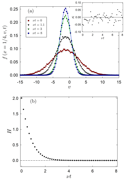
Figure 2: (Color online) Relaxation towards the USF state. The initial condition is Gaussian, centered in $u_{\text{st}}(x)$ and with variance $T=7\,T_{\text{st}}$. (a) Velocity distribution function at $x=1/4$ for $4$ different times. In the inset, the evolution of the excess kurtosis is shown. (b) Monotonic relaxation of the $H$ functional, in clear agreement with the proven $H$-theorem. Data is averaged over $6000$ trajectories in a system with $N=660$ sites, $\nu=20$, and $a=5$. Solid lines correspond to the (theoretical) Gaussian distributions for the plotted times, except for the last time in which it represents the theoretical steady distribution.

Secondly, we study the relaxation to the USF state from another initial preparation, for which the velocity profile $u(x,0)$ is different from the stationary but $T(x,0)=T_{\text{st}}$. The numerical results are shown in Fig. 3, and for the sake of simplicity we use again an initial Gaussian distribution. Specifically, we use $u(x,0)=u_{\text{st}}(x)+4.4\,\sin(2\pi x)$. Here, the departure from the Gaussian shape is evident, and thus we have not plotted the kurtosis. Consistently with our theoretical prediction, we get again a monotonous relaxation of $H$ towards its null stationary value.

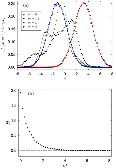
Figure 3: (Color online) The same plots as in Fig. 2, but starting from a different initial condition. Now, the initial PDF is a Gaussian centered in $u(x,0)=u_{\text{st}}(x)+4.4\,\sin(2\pi x)$ and with variance $T(t=0)=T_{\text{st}}$. In (a), solid lines correspond to the theoretical PDFs for the initial time and the steady state. In (b), $H$ decreases again monotonically towards its steady value, consistently with our theoretical prediction.

Finally, we consider situations for which the above presented proof is not rigorously applicable. As stated before, the Gram-Charlier series does not converge when the tails of the distribution decay to zero slower than the square root of the Gaussian. Nevertheless, when all the coefficients $\gamma_{n}$ defined in Eq. (46) exist and are finite, we still expect the $H$-theorem to hold. We illustrate this situation with an initial exponential distribution; specifically, we consider

$$f(x,v,0)=\frac{1}{\sqrt{2T(t=0)}}\exp\left[\frac{\sqrt{2}\left|v-u(x,t=0)\right|}{\sqrt{T(t=0)}}\right],$$ (50)

with $u(x,t=0)=u_{\text{st}}(x)+4.4\sin(2\pi x)$ and $T(t=0)=0.1\,T_{\text{st}}$. Consistently with our expectation, we can see in Fig. 4 that indeed the $H$-functional also monotonically decreases.

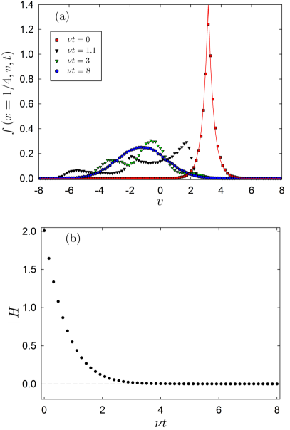
Figure 4: (Color online) The same plots as in Fig. 2, but starting from an initial PDF with a divergent Gram-Charlier series. Concretely, the plots correspond to an exponential initial distribution centered in $u(x,t=0)=u_{\text{st}}(x)+4.4\,\sin(2\pi x)$ and with $T(t=0)=0.1\,T_{\text{st}}$.

V.2 Numerical results in the uniformly heated system

To conclude, we put forward the results of simulations for the uniformly heated system. Specifically, our simulations have been done for $\nu=20$, $a=0$ (no shear) and $\xi=50$. In order not to overload the reader with too many examples, we only present the more complex case in Fig. 5: the relaxation towards the steady state from an initial exponential distribution, as given by Eq. (50). In particular, we consider that $u(x,t=0)=4.4\,\sin(2\pi x)$ and $T(t=0)=0.1\,T_{\text{st}}$. Note that the perturbation from the steady values is the same as in Fig. 4 for the sheared case. Again, we observe the monotonic relaxation of $H$ towards the stationary value, consistently with our theoretical result, even for a initial distribution for which the Gram-Charlier series does not converge.

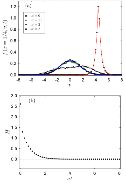
Figure 5: (Color online) Numerical results for the uniformly heated system. The plots are analogous to those in Fig. 2, (a) time evolution of the PDF and (b) time evolution of the $H$-functional. The system is initially prepared with an exponential PDF centered in $u(x,t=0)=4.4\,\sin(2\pi x)$ and with $T(t=0)=0.1\,T_{\text{st}}$. Data is averaged over $3000$ trajectories in a system with $N=330$ sites.

VI Conclusions

Within a simplified model for a granular-like velocity field, we have analytically shown that the nonequilibrium steady state that the system eventually reaches in the long time limit is globally stable. This has been done for quite a general situation, in which energy may be injected into the system both through the boundaries and by a heating mechanism that acts in the bulk. The proof is valid both for spatially homogeneous situations (such as the uniformly heated system) and inhomogeneous situations (such as the USF or Couette states).

The proof of global stability is based on showing that the $H$-functional $H=\int\!dx\,dv\,f\ln(f/f_{\text{st}})$ (the Kullback-Leibler divergence between the time evolving one-particle PDF $f(x,v,t)$ and its value in the stationary state $f_{\text{st}}(x,v)$ Cover and Thomas (2006)) is non-increasing in the infinite time limit. Thus, we do not need $H$ to be a “good” Lyapunov functional for all times in order to prove global stability. In conclusion, global stability and the validity of an $H$-theorem do not seem to be unavoidably tied.

Moreover, we have analytically shown that the Boltzmann functional $H_{B}=\int\!dx\,dv\,f\ln f$ cannot be, in general, a Lyapunov functional for systems with non-conservative interactions. Close to the steady state, we have proven that $dH_{B}/dt$ contains non-vanishing terms that are linear in the deviations $\Delta f=f-f_{\text{st}}$. Therefore, a reversal of the sign of $\Delta f$ entails a reversal of the sign of $dH_{B}/dt$. This general analytical proof on the inadequacy of $H_{B}$ as a Lyapunov functional is in agreement with previous results in some specific cases Bena et al. (2006); Marconi et al. (2013).

We have also succeeded in demonstrating that the $H$-functional is non-increasing and thus a “good” Lyapunov functional for some specific driving mechanisms. Our proof is not restricted to spatially homogeneous situations and is applicable to two relevant physical cases: the approach to (i) the USF state and (ii) the NESS corresponding to the uniformly heated case. The proof involves a suitable expansion of the one-particle PDF in Hermite polynomials, which is a generalisation of the well-known Sonine-Laguerre expansion in kinetic theory. Although the proof is only rigorous for PDFs having a convergent series expansion, we expect it to remain valid for more general PDFs. In fact, we have numerically validated this expectation in some specific situations.

The analytical results presented here are thus in agreement with the numerical evidence in Refs. Marconi et al. (2013); García de Soria et al. (2015) and advance the understanding of this field in a twofold way. First, an analytical proof, which was lacking, is provided for a simplified model. Second, spatially inhomogeneous situations are considered, both in the time evolution and in its steady state.

Some limitations of our results have to be underlined, though. First, the simplifications introduced in the model make it impossible to address the problem of the stability of the homogeneous cooling state in the undriven system at the level of the kinetic equation, as already discussed in Ref. Manacorda et al. (2016). Second, for the driving mechanisms for which we can analytically prove that $H$ is a “good” Lyapunov functional, the steady distribution is exactly Gaussian. Nevertheless, we think that this is not a fundamental point and expect that the kind of expansion-based proof presented here may be extended to other situations. A particularly appealing case is the approach to the Couette NESS, for which the stationary PDF is non-Gaussian in the model Manacorda et al. (2016).

On a different note, our kinetic equation (14) shows some resemblance to evolution equations for the one-particle PDF found in other physical contexts, such as the Vlasov equation in plasma physics or astrophysics Chavanis et al. (1996); Chavanis (1998); Yamaguchi et al. (2004) or the non-linear (in the distribution function) Fokker-Planck equation for systems of infinitely many coupled non-linear oscillators exhibiting phase transitions Desai and Zwanzig (1978). It is a drift-like term depending on a certain average of the PDF that all these different problems share. Both for the Vlasov and the non-linear Fokker-Planck equations, the existence of a Lyapunov functional has been proved by considering a variant of the functional $H[f]$ defined in Eq. (4) Shiino (1985, 1987); Bonilla et al. (1996). Thus, an interesting prospect is to investigate if this kind of approach may be extended to our class of models with non-conservative interactions.

Our work also opens the door to applying the ideas developed in this paper to more complex models, closer to real non-conservative systems, like granular gases. The pioneering numerical work in Refs. Marconi et al. (2013); García de Soria et al. (2015) strongly suggests that the $H$-functional is a “good” Lyapunov functional for granular fluids. It seems worth trying to analytically prove that this is indeed the case for the inelastic Boltzmann equation, at least for some specific situations. If nothing else, one would like to be able to show that the long time solutions are globally stable by showing that $H$ is asymptotically non-increasing, similarly to what has been done here.

Appendix A Derivation of the expression for $dH/dt$ in a general driven state

Let us consider the three contributions to $dH/dt$ in Eq. (29). We start with the diffusive one,

$$\left.\frac{dH}{dt}\right|_{\text{diff}}=\int\!\!dx\,dv\,\mathcal{L}_{\text{diff}}f\,\ln\left(\frac{f}{f_{\text{st}}}\right)-\int\!\!dx\,dv\,\frac{f}{f_{\text{st}}}\,\mathcal{L}_{\text{diff}}f_{\text{st}},$$ (51)

where $\mathcal{L}_{\text{diff}}f=\partial_{x}^{2}{f}$ and we have used that $\int\!\!dx\,dv\,\partial_{x}^{2}{f_{\text{st}}}$ vanishes identically. Integrating by parts the first term on the rhs of Eq. (51), the result is

$$\int\!\!dv\,\partial_{x}{f}\left.\ln\left(\frac{f}{f_{\text{st}}}\right)\right|_{0}^{1}-\int\!\!dx\,dv\,f\partial_{x}{\ln f}\left(\partial_{x}{\ln f}-\partial_{x}{\ln f_{\text{st}}}\right).$$ (52)

Also integrating by parts the second term, one obtains

$$-\int\!\!dv\,\left.\frac{f}{f_{\text{st}}}\partial_{x}{f_{\text{st}}}\right|_{0}^{1}+\int\!\!dx\,dv\,f\partial_{x}{\ln f_{\text{st}}}\left(\partial_{x}{\ln f}-\partial_{x}{\ln f_{\text{st}}}\right).$$ (53)

We assume that the boundary terms are equal to zero, that is,

$$\int\!\!dv\,\left[\partial_{x}{f}\ln\left(\frac{f}{f_{\text{st}}}\right)-\frac{f}{f_{\text{st}}}\partial_{x}{f_{\text{st}}}\right]_{0}^{1}=0.$$ (54)

This is obviously true for Lees-Edwards and periodic boundary conditions . Summing the two contributions to the diffusive term above, we have

$$\left.\frac{dH}{dt}\right|_{\text{diff}}=-\int\!\!dx\,dv\,f\left(\partial_{x}{\ln f}-\partial_{x}{\ln f_{\text{st}}}\right)^{2},$$ (55)

which is Eq. (30) of the main text.

The noise term is treated along the same lines as above, but integrating by parts in $v$ instead of $x$, since $\mathcal{L}_{\text{noise}}f=\frac{\xi}{2}\partial_{v}^{2}{f}$. There in, the boundary terms vanish if $f$ and $f_{\text{st}}$ tend to zero fast enough for $v\to\pm\infty$, and

$$\left.\frac{dH}{dt}\right|_{\text{noise}}=-\frac{\xi}{2}\int\!\!dx\,dv\,f\left(\partial_{v}{\ln f}-\partial_{v}{\ln f_{\text{st}}}\right)^{2},$$ (56)

which is Eq. (32).

Now we focus on the inelastic contribution,

$$\left.\frac{dH}{dt}\right|_{\text{inel}}=\int\!\!dx\,dv\,\mathcal{L}_{\text{inel}}f\,\ln\left(\frac{f}{f_{\text{st}}}\right)-\int\!\!dx\,dv\,\frac{f}{f_{\text{st}}}\,\mathcal{L}_{\text{inel}}f_{\text{st}},$$ (57)

in which $\mathcal{L}_{\text{inel}}f=\frac{\nu}{2}\partial_{v}{[(v-u)f]}$. Then,

$$\left.\frac{dH}{dt}\right|_{\text{inel}}= \;\frac{\nu}{2}\int\!\!dx\,dv\,\partial_{v}{[(v-u)f]}\,\ln\left(\frac{f}{f_{\text{st}}}\right)$$

$$-\frac{\nu}{2}\int\!\!dx\,dv\,\partial_{v}{[(v-u_{\text{st}})f_{\text{st}}]}\,\frac{f-f_{\text{st}}}{f_{\text{st}}}.$$ (58)

Again, integrating by parts in $v$ (here we do not write the boundary terms at $v\to\pm\infty$), the first term on the rhs of Eq. (58) is

$$-\frac{\nu}{2}\int\!\!dx\,dv\,(v-u)f\,\left(\partial_{v}{\ln f}-\partial_{v}{\ln f_{\text{st}}}\right),$$ (59)

whereas the second term gives

$$\frac{\nu}{2}\int\!\!dx\,dv\,(v-u_{\text{st}})f\,\left(\partial_{v}{\ln f}-\partial_{v}{\ln f_{\text{st}}}\right).$$ (60)

Summing up these two contributions, and taking into account that both $u$ and $u_{\text{st}}$ do not depend on $v$,

$$\left.\frac{dH}{dt}\right|_{\text{inel}}=\frac{\nu}{2}\int\!\!dx\,(u-u_{\text{st}})\int\!\!dv\,f\left(\partial_{v}{\ln f}-\partial_{v}{\ln f_{\text{st}}}\right)$$ (61)

Since $\int\!dv\,f\,\partial_{v}{\ln f}\equiv\int\!dv\,\partial_{v}{f}=0$, this leads to Eq. (31).

Appendix B Simulation strategy

In the simulations, so as to generate a trajectory of the stochastic process, we proceed as follows. (i) A pair $(l,l+1)$ is chosen at random and undergoes the inelastic collision described by Eq. (5), (ii) all the particles are submitted to the stochastic thermostat according to (6) and (7), and (iii) time is incremented by $\delta\tau=-(N\omega)^{-1}\ln x$, with $x$ being a homogeneously distributed random number in $(0,1)$ Bortz et al. (1975); Gillespie (1976); Prados et al. (1997); Serebrinsky (2011). This cycle (random choice of a pair and noise interaction followed by a time increment) is repeated until time exceeds some maximum time $t_{\text{max}}$.

Regarding the measurements of $f(x,v,t)$, we sample both position and velocity spaces by defining $N_{x}$ bins of width $\Delta x$ and $N_{v}$ bins of with $\Delta v$. Of course, the product $N_{x}\Delta x=1$, the whole lattice, whereas $N_{v}\Delta v$ gives the range of velocities bounded by the cutoffs $v_{\text{\text{min}}}$ and $v_{\text{max}}$. In our simulations, we control that the contribution to the PDFs coming from velocities outside the considered interval $[v_{\text{min}},v_{\text{max}}]$ is negligible. With such a binning, we build up an histogram and therefrom the distribution function $f(x,v,t)$, which is represented by a $N_{x}\times N_{v}$ matrix for each time $t$. Both $H$ and $H_{B}$ are computed by numerically replacing the integral over $x$ and $v$ with sums over the prescribed bins.

Appendix C Derivation of Eq. (47)

In order to derive Eq. (47), we have to substitute the Gaussian stationary solution (43) and the Gram-Charlier series (44) into the three contributions to $dH/dt$, given by Eqs. (30), (31) and (32).

For the inelastic term, it is readily obtained that

$$\left.\frac{dH}{dt}\right|_{\text{inel}}=\frac{\nu}{2T_{\text{st}}}\int\!\!dx\left(u-u_{\text{st}}\right)^{2}.$$ (62)

For the diffusive and noise terms, the key ideas are a changing the integration over velocities from $v$ to $c=(v-u)/\sqrt{T}$ and the use of the recursion relations and the orthogonality property of the Hermite polynomials Abramowitz and Stegun (1972). Working along these guidelines, we arrive at

$$\left.\frac{dH}{dt}\right|_{\text{diff}} = -\int\!\!dx\,T\left(\frac{u^{\prime}}{T}-\frac{u_{\text{st}}^{\prime}}{T_{\text{st}}}\right)^{2}$$ (63)

$$-\frac{u_{\text{st}}^{\prime 2}}{T_{\text{st}}^{2}}\int\!\!dx\left(u-u_{\text{st}}\right)^{2}+B_{1}(t),$$

$$\left.\frac{dH}{dt}\right|_{\text{noise}} = -\frac{\xi}{2}\int\!\!dx\,T\left(\frac{1}{T}-\frac{1}{T_{\text{st}}}\right)^{2}$$ (64)

$$-\frac{\xi}{2T_{\text{st}}^{2}}\int\!\!dx\left(u-u_{\text{st}}\right)^{2}+B_{2}(t),$$

where $B_{1}$ and $B_{2}$ are, respectively, the first and the second term in Eq. (49). The sum of the factors multiplying $\int\!\!dx\left(u-u_{\text{st}}\right)^{2}$ vanishes by taking into account the equation for the (spatially homogeneous) stationary temperature. Therefore, the sum of the remaining terms leads right to Eq. (47).

References

- Lyapunov (1992) A. M. Lyapunov, Int. J. Cont. 55, 531 (1992).
- Boltzmann (1995) L. Boltzmann, Lectures on Gas Theory (Dover, 1995).
- Lebowitz (1993a) J. L. Lebowitz, Phys. Today 46, 32 (1993a).
- Lebowitz (1993b) J. L. Lebowitz, Physica A 194, 1 (1993b).
- Chapman and Cowling (1970) S. Chapman and T. G. Cowling, The Mathematical Theory of Non-Uniform Gases, 3rd ed. (Cambridge University Press, Cambridge, UK, 1970).
- Van Kampen (1992) N. G. Van Kampen, Stochastic processes in physics and chemistry, Vol. 1 (Access Online via Elsevier, 1992).
- Marconi et al. (2013) U. M. B. Marconi, A. Puglisi, and A. Vulpiani, J. Stat. Mech. , P08003 (2013).
- García de Soria et al. (2015) M. I. García de Soria, P. Maynar, S. Mischler, C. Mouhot, T. Rey, and E. Trizac, J. Stat. Mech. , P11009 (2015).
- Pöschel and Luding (2001) T. Pöschel and S. Luding, eds., Granular Gases, Lecture Notes in Physics, Vol. 564 (Springer, Berlin, 2001).
- Villani (2006) C. Villani, J. Stat. Phys. 124, 781–822 (2006).
- Bena et al. (2006) I. Bena, F. Coppex, M. Droz, P. Visco, E. Trizac, and F. van Wijland, Physica A 370, 179 (2006).
- Baldassarri et al. (2002) A. Baldassarri, U. Marini Bettolo Marconi, and A. Puglisi, EPL 58, 14 (2002).
- Lasanta et al. (2015) A. Lasanta, A. Manacorda, A. Prados, and A. Puglisi, New J. Phys. 17, 083039 (2015).
- Manacorda et al. (2016) A. Manacorda, C. A. Plata, A. Lasanta, A. Puglisi, and A. Prados, J. Stat. Phys. 164, 810 (2016).
- Plata et al. (2016) C. A. Plata, A. Manacorda, A. Lasanta, A. Puglisi, and A. Prados, J. Stat. Mech. , 093203 (2016).
- Prasad et al. (2017) V. V. Prasad, S. Sabhapandit, A. Dhar, and O. Narayan, Phys. Rev. E 95, 022115 (2017).
- Kac (1956) M. Kac, in Proc. 3rd Berkeley Symp. Mathematics Statistics Probability, Vol. 3 (Berkeley, CA: University of California Press, 1956) p. 171.
- Brey and Prados (1993) J. J. Brey and A. Prados, Phys. Rev. E 47, 1541 (1993).
- Brey and Prados (1994) J. J. Brey and A. Prados, Phys. Rev. B 49, 984 (1994).
- Brey et al. (1994) J. J. Brey, A. Prados, and M. J. Ruiz-Montero, J. Non-Cryst. Solids 172, 371 (1994).
- Vlad and Ross (1997) M. O. Vlad and J. Ross, J. Phys. Chem. B 101, 8756 (1997).
- Vlad et al. (1998) M. O. Vlad, F. Moran, and J. Ross, J. Phys. Chem. B 102, 4598 (1998).
- Prados et al. (2000) A. Prados, J. J. Brey, and B. Sánchez-Rey, Physica A 284, 277 (2000).
- Earnshaw and Keener (2010) B. Earnshaw and J. Keener, SIAM J. Appl. Dyn. Syst. 9, 220 (2010).
- Van Noije and Ernst (1998) T. P. C. Van Noije and M. H. Ernst, Granul. Matter 1, 57 (1998).
- Montanero and Santos (2000) J. M. Montanero and A. Santos, Granul. Matter 2, 53 (2000).
- García de Soria et al. (2009) M. I. García de Soria, P. Maynar, and E. Trizac, Mol. Phys. 107, 383 (2009).
- García de Soria et al. (2012) M. I. García de Soria, P. Maynar, and E. Trizac, Phys. Rev. E 85, 051301 (2012).
- Pagonabarraga et al. (2002) I. Pagonabarraga, E. Trizac, T. P. C. van Noije, and M. H. Ernst, Phys. Rev. E 65, 011303 (2002).
- Maynar et al. (2009) P. Maynar, M. I. García de Soria, and E. Trizac, Eur. Phys. J. Spec. Top. 179, 123 (2009).
- Prados and Trizac (2014) A. Prados and E. Trizac, Phys. Rev. Lett. 112, 198001 (2014).
- Trizac and Prados (2014) E. Trizac and A. Prados, Phys. Rev. E 90, 012204 (2014).
- Prasad et al. (2013) V. V. Prasad, S. Sabhapandit, and A. Dhar, EPL 104, 54003 (2013).
- Ben-Naim and Krapivsky (2003) E. Ben-Naim and P. L. Krapivsky, in Granular Gas Dynamics, Lecture Notes in Physics, Vol. 624, edited by T. Pöschel and N. Brilliantov (Springer, Berlin, 2003) pp. 65–94.
- Note (1) This kind of Fokker-Planck kernel is similar to the one appearing in the Fokker-Planck equation for biomolecules in which their total length , where is the length of each of the modules of the molecule, is controlled and kept constant. This is quite logical, since in both situations there is an additive conservation law: here it is the total momentum that is conserved, whereas in biomolecules the constant of motion is the total length Bonilla et al. (2015).
- Note (2) Note that the density of the model is fixed, there is no mass transport in the system.
- Kipnis et al. (1982) C. Kipnis, C. Marchioro, and E. Presutti, J. Stat. Phys. 27, 65 (1982).
- Prados et al. (2011) A. Prados, A. Lasanta, and P. I. Hurtado, Phys. Rev. Lett. 107, 140601 (2011).
- Prados et al. (2012) A. Prados, A. Lasanta, and P. I. Hurtado, Phys. Rev. E 86, 031134 (2012).
- Hurtado et al. (2013) P. I. Hurtado, A. Lasanta, and A. Prados, Phys. Rev. E 88, 022110 (2013).
- Lasanta et al. (2016) A. Lasanta, P. I. Hurtado, and A. Prados, Eur. Phys. J. E 39, 35 (2016).
- Lees and Edwards (1972) A. W. Lees and S. F. Edwards, J. Phys. C 5, 1921 (1972).
- Chebyshev (1890) P. L. Chebyshev, Acta Math. 14, 305 (1890).
- Charlier (5 06) C. V. L. Charlier, Ark. Math. Astr. och Phys. 2, 1 (1905-06).
- Edgeworth (1905) F. Y. Edgeworth, Cambridge Philos. Soc. 20, 36 (1905).
- Wallace (1958) D. L. Wallace, Ann. Math. Stat. 29, 635 (1958).
- Abramowitz and Stegun (1972) M. Abramowitz and I. A. Stegun, eds., Handbook of Mathematical Functions (Dover, New York, 1972).
- Cramér (1925) H. Cramér, in Proceedings of the Sixth Scandinavian Congress of Mathematicians, Copenhagen (1925) pp. 399–425.
- Szegö (1939) G. Szegö, Amer. Math. Soc. 23 (1939).
- Cover and Thomas (2006) T. M. Cover and J. M. Thomas, Elements of Information Theory (New York: Wiley, 2006).
- Chavanis et al. (1996) P.-H. Chavanis, J. Sommeria, and R. Robert, Astrophys. J. 471, 385 (1996).
- Chavanis (1998) P.-H. Chavanis, Ann. N. Y. Acad. Sci. 867, 120 (1998).
- Yamaguchi et al. (2004) Y. Y. Yamaguchi, J. Barré, F. Bouchet, T. Dauxois, and S. Ruffo, Physica A 337, 36 (2004).
- Desai and Zwanzig (1978) R. C. Desai and R. Zwanzig, J. Stat. Phys. 19, 1 (1978).
- Shiino (1985) M. Shiino, Physics Letters A 112, 302 (1985).
- Shiino (1987) M. Shiino, Phys. Rev. A 36, 2393 (1987).
- Bonilla et al. (1996) L. L. Bonilla, J. A. Carrillo, and J. Soler, Phys. Lett. A 212, 55 (1996).
- Note (3) For the Couette state, in which the PDF at the boundaries is Gaussian with zero average velocity and a given temperature for all times, the first term is identically zero and the second vanishes because for all .
- Bortz et al. (1975) A. B. Bortz, M. H. Kalos, and J. L. Lebowitz, J. Comput. Phys. 17, 10 (1975).
- Gillespie (1976) D. T. Gillespie, J. Comput. Phys. 22, 403 (1976).
- Prados et al. (1997) A. Prados, J. J. Brey, and B. Sánchez-Rey, J. Stat. Phys. 89, 709 (1997).
- Serebrinsky (2011) S. A. Serebrinsky, Phys. Rev. E 83, 037701 (2011).
- Bonilla et al. (2015) L. L. Bonilla, A. Carpio, and A. Prados, Phys. Rev. E 91, 052712 (2015).