Virtual photon polarization in ultrarelativistic heavy-ion collisions

Abstract

The polarization of direct photons produced in an ultrarelativistic heavy-ion collision reflects the momentum anisotropy of the quark-gluon plasma created in the collision. This paper presents a general framework, based on the photon spectral functions in the plasma, for analyzing the angular distribution and thus the polarization of dileptons in terms of the plasma momentum anisotropies. The rates of dilepton production depend, in general, on four independent spectral functions, corresponding to two transverse polarizations, one longitudinal polarization, and – in plasmas in which the momentum anisotropy is not invariant under parity in the local rest frame of the matter – a new spectral function, $\rho_{n}$, related to the anisotropy direction in the collision. The momentum anisotropy appears in the difference of the two transverse spectral functions, as well as in $\rho_{n}$. As an illustration, we delineate the spectral functions for dilepton pairs produced in the lowest order Drell-Yan process of quark-antiquark annihilation to a virtual photon.

I Introduction

Direct photons, both real and virtual, are an important probe of the dynamics of ultrarelativistic heavy-ion collisions. An average temperature of the quark-gluon plasma (QGP) formed in high-energy collisions has been extracted from the transverse momentum spectrum of direct photons in the range $q_{\rm T}\sim$ 1-3 GeV PHENIX ; STAR ; ALICE . Theoretically, measurements of the photon polarization through the angular distribution of dileptons ($l^{+}\l^{-}$) have been proposed to provide information on the early stages of collisions, before the onset of thermalization Hoyer ; Bratkovskaya ; Shuryak . While relativistic hydrodynamics provides a successful spacetime description of the later stages of the collision dynamics and associated hadronic and leptonic observables QM2015_proc , important questions concerning the early dynamics, such as the degree of thermalization as well as isotropization of the QGP, have not been answered either experimentally or theoretically. Recently, Ref. BH proposed using the polarization of direct photons as a measure of the gluon anisotropy in collisions. While measuring direct photon polarization, involving external conversion to dilepton pairs, is very difficult experimentally, a more promising approach to is measure polarization of virtual photons, through the angular distribution of dileptons produced via internal conversion.

The lowest order mechanism to produce dilepton pairs is the Drell-Yan process, Fig. 1, in which a quark and an antiquark annihilate to a virtual photon. The dilepton cross section $d\sigma/d\Omega$ can be parametrized as $\propto 1+\lambda\cos^{2}\theta+\mu\sin 2\theta\cos\phi+(\nu/2)\sin^{2}\theta\cos 2\phi$, where $\theta$ and $\phi$ are the polar and azimuthal angles of one of the dileptons in the dilepton rest frame measured in the Collins-Soper reference frame Collins-Soper ; Lam-Tung . High-energy $p\bar{p}$ and $pp$ collisions at the Tevatron and the LHC have confirmed the leading-order prediction $\lambda\simeq 1$, $\mu=\nu=0$, for $q_{\rm T}\mathrel{\hbox to0.0pt{\raise 2.20013pt\hbox{$<$}\hss}{\lower 2.20013pt\hbox{$\sim$}}}$ 5 GeV and invariant dilepton mass $M_{l^{+}l^{-}}\simeq M_{Z}$ (see, e.g., Peng and references therein). The dilepton angular distribution in In-In collisions has been measured by the NA60 experiment NA60 at the CERN-SPS in the primary kinematical range $0.4<M_{l^{+}l^{-}}<$ 0.9 GeV, in which production of dileptons by hadronic sources such as $\pi^{+}\pi^{-}$ annihilation dominates Drell-Yan dileptons; the results are consistent with $\lambda=\mu=\nu=0$.

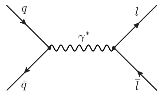
Figure 1: Lowest order Drell-Yan production of a lepton pair.

On the other hand, in ultrarelativistic heavy-ion collisions we expect the momentum-space anisotropy of the QGP to be detected most readily in dilepton production in the range 1 GeV $<q_{\rm T}<$ 3 GeV and $M_{l^{+}l^{-}}\mathrel{\hbox to0.0pt{\raise 2.20013pt\hbox{$<$}\hss}{\lower 2.20013pt\hbox{$\sim$}}}0.3$ GeV where the excess of direct photons is seen experimentally PHENIX . In this paper, we present a general framework for analyzing the angular distribution of dileptons emitted from a QGP, which can be used to extract quark and gluon momentum anisotropies in the collision. The basic starting point is the photon polarization tensor and associated spectral function; we analyze the spectral function in terms of four vectors, two transverse polarization vectors, a longitudinal polarization vector, and a vector specifying the momentum anisotropy. Such a decomposition combined with the leptonic tensor describing the conversion of a virtual photon into a dilepton pair leads to a general formula relating the momentum anisotropy of the plasma and the dilepton angular distribution. As an illustration, we apply the formalism to virtual photon emission through the leading-order Drell-Yan process in a plasma with anisotropic distributions of the Romatschke-Strickland form RS .

II Dilepton production

Quite generally, the production rate, $R$, of a dilepton pair is proportional to the spectral function, $\rho_{\mu\nu}$, of the in-medium photon polarization or self-energy operator, for momentum $\vec{q}$ and energy $q^{0}$,

$$\Pi_{\mu\nu}(\vec{q}\,,z)=e^{2}\int_{-\infty}^{\infty}\frac{dq^{0}}{2\pi}\frac{\rho_{\mu\nu}(\vec{q}\,,q^{0})}{z-q^{0}}\,,$$ (1)

times the squared matrix element $L^{\mu\nu}$ (L for leptons) for a virtual photon of 4-momentum $q$ to produce a lepton of 4-momentum $p$ and mass $m$ and an antilepton of 4-momentum $p^{\prime}$, averaged over the spins of the leptons. Explicitly,

$$\frac{dR_{l^{+}l^{-}}}{d^{3}\bar{p}d^{3}\bar{p}^{\prime}}=\frac{\alpha^{2}}{4\pi^{4}Q^{4}}\ \rho_{\mu\nu}(q)L^{\mu\nu}(p,p^{\prime})\,,$$ (2)

with the leptonic tensor,

$$L_{\mu\nu}(q,s)=2\left(q_{\mu}q_{\nu}-g_{\mu\nu}Q^{2}-s_{\mu}s_{\nu}\right),$$ (3)

where $d^{3}\bar{p}\equiv d^{3}p/2E_{p}$, $d^{3}\bar{p}^{\prime}\equiv d^{3}p^{\prime}/2E_{p^{\prime}}$, $q=p+p^{\prime}$, $s=p-p^{\prime}$, $Q^{2}\equiv q^{\mu}q_{\mu}>0$, and $Q^{2}+s^{2}=4m^{2}$ with $m$ the lepton mass.

The spectral function $\rho_{\mu\nu}(q)$ is related to the cut, or imaginary part, of the photon polarization operator, illustrated in Fig 2. Its explicit form in the kinematical regime $q^{0}\gg T\gg\sqrt{Q^{2}}$ has been previously evaluated using hard thermal loop effective theory for the isotropic quark-gluon plasma Carrington:2007gt ; Laine:2015iia . The heart of the problem in this paper is to determine the structure of $\rho_{\mu\nu}(q)$, to see how the anisotropy of the gluon and quark distributions is reflected in the final orientation of the dilepton pair.

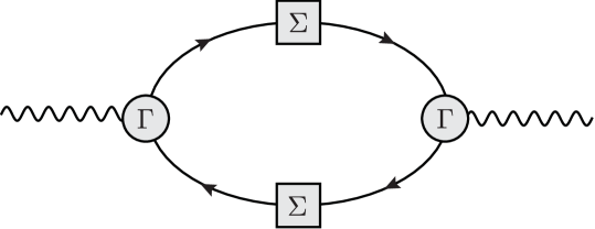
Figure 2: Photon polarization tensor with hard thermal loop corrections to the quark lines and vertices Carrington:2007gt .

III Structure of $\rho_{\mu\nu}$

In a heavy-ion collision volume, the initial gluon and quark distributions are anisotropic in momentum space with a single preferred axis $\hat{n}$, which we assume to be along the beam direction Strickland:2013uga (we do not consider at this point possible multiple anisotropy axes). We define the four vector $n^{\mu}$ to have space component $\hat{n}$ in the local rest frame of the matter and time component, $n^{0}=0$,

$$n^{\mu}=(0,\hat{n})\,,$$ (4)

so that $n^{2}=-1$. We also define, in the local rest frame, the two transverse polarization vectors

$$\varepsilon_{i}^{\mu}=(0,\hat{\varepsilon}_{i})\,,$$ (5)

where $\hat{\varepsilon}_{1}\equiv(\vec{q}\times\hat{n})\times\vec{q}/|\vec{q}\times\hat{n}|$ and $\hat{\varepsilon}_{2}\equiv\vec{q}\times\hat{n}/|\vec{q}\times\hat{n}|$. These polarization vectors are illustrated in the left panel of Fig. 3. In addition, we define the longitudinal polarization vector

$$\varepsilon_{\rm L}^{\mu}\equiv\frac{1}{\sqrt{Q^{2}}}(|\vec{q}\,|,q^{0}\hat{q})=(|\vec{\tilde{q}}\,|,\tilde{q}^{0}\hat{q})\,.$$ (6)

where we write $\tilde{q}^{\mu}=q^{\mu}/\sqrt{Q^{2}}$. Note that $\varepsilon_{1}^{2}=\varepsilon_{2}^{2}=\varepsilon_{\rm L}^{2}=-1$. The three polarization vectors are individually orthogonal to $q^{\mu}$: $(q\varepsilon)=0$ (where $(ab)$ denotes the four vector product of $a$ and $b$) and together with $q^{\mu}$ form an orthogonal basis obeying;

$$g^{\mu\nu}=\tilde{q}^{\mu}\tilde{q}^{\nu}-\varepsilon_{1}^{\mu}\varepsilon_{1}^{\nu}-\varepsilon_{2}^{\mu}\varepsilon_{2}^{\nu}-\varepsilon_{\rm L}^{\mu}\varepsilon_{\rm L}^{\nu}\,.$$ (7)

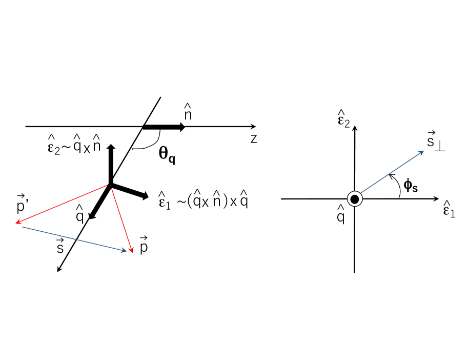
Figure 3: (Left) Virtual photon polarization vectors $\hat{\varepsilon}_{i}$ and the relative spatial momentum $\vec{s}$ between the lepton and antilepton. (Right) The relative lepton momentum in the plane transverse to the virtual photon momentum $\vec{q}$.

Thus the photon spectral function, $\rho_{\mu\nu}$, is a sum of terms of the form

$$a\varepsilon_{\rm L}^{\mu}\varepsilon_{\rm L}^{\nu}+b\varepsilon_{1}^{\mu}\varepsilon_{1}^{\nu}+c(\varepsilon_{1}^{\mu}\varepsilon_{\rm L}^{\nu}+\varepsilon_{\rm L}^{\mu}\varepsilon_{1}^{\nu})+d\varepsilon_{2}^{\mu}\varepsilon_{2}^{\nu}\,.$$ (8)

There are no terms proportional to $q^{\mu}q^{\nu}$ for $Q^{2}\neq 0$, since $q$ is a zero eigenvector of $\rho$; in addition $(n\varepsilon_{2})=0$, so there are no $\varepsilon_{2}\varepsilon_{\rm L}$ terms by symmetry. Since $\vec{n}$ can be written as the linear superposition, $\vec{n}=\cos\theta_{q}\hat{q}+\sin\theta_{q}\vec{\varepsilon}_{2}$, with $\theta_{q}$ being the angle between $\hat{n}$ and $\hat{q}$, and $n^{0}=0$, we obtain

$$n^{\mu}=\cos\theta_{q}(\tilde{q}^{0}\varepsilon_{\rm L}^{\mu}-|\vec{\tilde{q}}\,|\tilde{q}^{\mu})+\sin\theta_{q}\,\varepsilon_{1}^{\mu}\,.$$ (9)

We also introduce the four-vector ${\cal N}^{\mu}$ with the property $({\cal N}q)=0$ as,

$${\cal N}^{\mu}\equiv\tilde{q}^{0}\,\cos\theta_{q}\,\varepsilon_{\rm L}^{\mu}+\sin\theta_{q}\,\varepsilon_{1}^{\mu}=n^{\mu}-(\tilde{q}n)\tilde{q}^{\mu},$$ (10)

Thus the $\varepsilon_{1}^{\mu}\varepsilon_{\rm L}^{\nu}+\varepsilon_{\rm L}^{\mu}\varepsilon_{1}^{\nu}$ term can be eliminated in favor of ${\cal N}^{\mu}{\cal N}^{\nu}$, $\varepsilon_{1}^{\mu}\varepsilon_{1}^{\nu}$, and $\varepsilon_{\rm L}^{\mu}\varepsilon_{\rm L}^{\nu}$. In addition, ${\cal N}^{2}=-(1+(n\tilde{q})^{2})$. The latter term, plus the explicit $\varepsilon_{\rm L}^{\mu}\varepsilon_{\rm L}^{\nu}$ term in Eq. (8), can be eliminated using Eq. (7). The photon spectral function, again with the help of Eq. (7), assumes the general form

$$\rho^{\mu\nu} = \varepsilon_{\rm L}^{\mu}\varepsilon_{\rm L}^{\nu}\rho^{\rm L}+\varepsilon_{1}^{\mu}\varepsilon_{1}^{\nu}\rho^{\rm T}_{1}+\varepsilon_{2}^{\mu}\varepsilon_{2}^{\nu}\rho^{\rm T}_{2}+{\cal N}^{\mu}{\cal N}^{\nu}\rho_{n}$$ (12)

$$= -(g^{\mu\nu}-\tilde{q}^{\mu}\tilde{q}^{\nu})\rho^{\rm L}+\varepsilon_{1}^{\mu}\varepsilon_{1}^{\nu}(\rho^{\rm T}_{1}-\rho^{\rm L})$$

$$+\varepsilon_{2}^{\mu}\varepsilon_{2}^{\nu}(\rho^{\rm T}_{2}-\rho^{\rm L})+{\cal N}^{\mu}{\cal N}^{\nu}\rho_{n}\,.$$

The momentum-space anisotropy of the system leads to the extra $\rho_{n}$ term, as well as a difference of $\rho_{1}^{\rm T}$ and $\rho_{2}^{\rm T}$.

The terms $\rho_{n}$, $\rho^{\rm T}_{2}$ can be extracted directly from Eqs. (12) and (10) as

$$\varepsilon_{1\,\mu}\rho^{\mu\nu}\varepsilon_{{\rm L}\,\nu}=-\tilde{q}\,^{0}\cos\theta_{q}\,\sin\theta_{q}\,\rho_{n}\,,$$ (13)

and

$$\varepsilon_{2\,\mu}\rho^{\mu\nu}\varepsilon_{2\,\nu}=\rho^{\rm T}_{2}\,,$$ (14)

while $\rho^{\rm L}$ is found from

$$\varepsilon_{{\rm L}\,\mu}\rho^{\mu\nu}\varepsilon_{{\rm L}\,\nu}=\rho^{\rm L}+(\tilde{q}\,^{0})^{2}\cos^{2}\theta_{q}\,\rho_{n}\,.$$ (15)

Using Eq. (13), we find $\rho_{1}^{\rm T}$ from the trace condition,

$$\rho^{\mu}_{\mu}=-(\rho^{\rm L}+\rho^{\rm T}_{1}+\rho^{\rm T}_{2}+(1+(n\tilde{q})^{2})\rho_{n})\,.$$ (16)

When the particle distribution functions are even under parity, so that $\vec{n}$ enters only as a special axis, not a special direction, the extra $\rho_{n}$ term must vanish. To see this we note that when the distribution functions are parity invariant, both parity and the transformation $\hat{n}\to-\hat{n}$ are independent symmetries, meaning that a parity transformation keeping $\vec{n}$ fixed is also a symmetry. But under such a transformation $\vec{\varepsilon}_{\rm L}$ transforms as a vector, while $\vec{\varepsilon}_{1}$ transforms as a pseudovector; thus the mixing of the two directions in $\rho_{ij}$, the source of $\rho_{n}$, cannot occur. For collisions of two identical nuclei, there should not be a special direction in the local rest frame of the matter. Below, when we write down the Drell-Yan rate in the medium in such a situation, we will see explicitly how this argument is realized. However, for asymmetric collisions, one expects a non-zero $\rho_{n}$ term in the photon spectral function. In the following, we keep the $\rho_{n}$ term in the general discussions.

The various $\rho$ depend separately on the local $q^{0}$, $q_{\perp}$, and $\vec{q}\cdot\hat{n}$, where $q_{\perp}$ is the magnitude of the component of $\vec{q}$ orthogonal to $\hat{n}$. Or expressed covariantly, they depend on $Q^{2}$, $(qu)$, as well as on $(qn)$, where $u_{\mu}$ is the 4-velocity of the local rest frame. Note that $(nu)\equiv 0$.

We look now at the eigenvalue structure of photon spectral function. In the local rest frame, in an isotropic system or for $\vec{q}$ along $\hat{n}$, the $\rho_{n}$ term vanishes and $\rho^{\rm T}_{1}=\rho^{\rm T}_{2}$, while for $\vec{q}\perp\hat{n}$ the eigenvectors of $\rho$ are the $\varepsilon_{i}$, with the two eigenvalues, $\rho^{\rm T}_{1}$ and $\rho^{\rm T}_{2}$. More generally, in the local rest frame, the eigenvectors of $\rho^{\mu\nu}$ are $q^{\mu}$ with eigenvalue 0, $\varepsilon_{2}^{\mu}$ with eigenvalue $\rho_{2}^{\rm T}$, and two orthogonal linear combinations of $\varepsilon_{1}^{\mu}$ and $\varepsilon_{\rm L}^{\mu}$ whose spatial components lie in the $(\vec{q},\hat{n})$ plane. In the isotropic limit, the eigenvector $\varepsilon_{\rm L}$ has eigenvalue $\rho_{\rm L}$, and $\varepsilon_{1}$ has eigenvalue $\rho_{\rm T}$. In contrast, when the system is anisotropic, the two eigenfunctions describe propagation in a birefringent medium with a mixing of the longitudinal (L) and transverse (T) polarizations. Furthermore, as $\vec{q}\to 0$, $\rho^{\rm T}_{i}-\rho^{\rm L}$ must vanish as $\vec{q}\,\,^{2}$, and thus, $\rho^{\rm T}_{i}=\rho^{\rm L}$ for $i=1,2$.

IV Emission rate of dileptons and photons

To calculate the production rates of dilepton pairs we first note that quite generally, $(sq)=0$, so that

$$\frac{1}{2}\rho^{\mu\nu}L_{\mu\nu} = -(Q^{2}\rho^{\mu}_{\mu}+s_{\mu}\rho^{\mu\nu}s_{\nu})$$ (18)

$$= Q^{2}\left(\rho^{\rm T}_{1}+\rho^{\rm T}_{2}+\rho_{n}\right)+4m^{2}\rho^{\rm L}$$

$$-s_{1}^{2}(\rho^{\rm T}_{1}-\rho^{\rm L})-s_{2}^{2}(\rho^{\rm T}_{2}-\rho^{\rm L})$$

$$+((qn)^{2}-(sn)^{2})\rho_{n}\,,$$

where we use the identity $Q^{2}+s^{2}=4m^{2}$, with $m$ being the lepton mass, and we define $s_{i}\equiv(s\varepsilon_{i})$ ($i=1,2$) to be the components of $\vec{s}$ transverse to $\vec{q}$ in the local rest frame: $\vec{s}_{\perp}=s_{1}\vec{\varepsilon}_{1}+s_{2}\vec{\varepsilon}_{2}$.

Equation (18) gives the dilepton production rate in terms of the projections of $s$ along the two transverse polarizations and $n$. The $s_{1}^{2}$ and $s_{2}^{2}$ terms contain the anisotropy produced by transverse virtual photons, while from Eq. (9), we see that the $s_{z}^{2}$ term arises from the mixing of longitudinal and transverse ($\vec{\varepsilon}_{1}$) virtual photons. As noted above, for symmetric collisions with parity invariance in the local matter rest frame, $\rho_{n}$ should vanish so then the final term Eq. (18) is absent. To bring out the anisotropic terms, we write $s_{1}=|{\vec{s}}_{\perp}|\cos\phi_{s}$, and $s_{2}=|{\vec{s}}_{\perp}|\sin\phi_{s}$; the squared matrix elements (18) become

$$\frac{1}{2}\rho^{\mu\nu}L_{\mu\nu} = 2Q^{2}\bar{\rho}^{\rm T}+\left(s_{\perp}^{2}+4m^{2}\right)\rho^{\rm L}$$ (19)

$$+\left(Q^{2}+(qn)^{2}-(sn)^{2}\right)\rho_{n}$$

$$-|\vec{s}_{\perp}|^{2}\left(\bar{\rho}^{\rm T}+\delta{\rho}^{\rm T}\cos 2\phi_{s}\right),$$

where $\bar{\rho}^{\rm T}\equiv(\rho_{1}^{\rm T}+\rho_{2}^{\rm T})/2$ and $\delta{\rho}^{\rm T}\equiv(\rho_{1}^{\rm T}-\rho_{2}^{\rm T})/2$. The $\cos 2\phi_{s}$ as well as the $\rho_{n}$ terms are anisotropic. For massless dileptons in the absence of $\rho_{n}$, the right side of Eq. (19) becomes $2Q^{2}\bar{\rho}^{\rm T}+|\vec{s}_{\perp}|^{2}(\rho^{\rm L}-\bar{\rho}^{\rm T}-\delta{\rho}^{\rm T}\cos 2\phi_{s})$. With $\theta_{s}$ the angle between $\vec{q}$ and $\vec{s}$, we see that this expression is of the form $\propto 1+\lambda_{s}\cos^{2}\theta_{s}+\mu_{s}\sin 2\theta_{s}\cos\phi_{s}+(\nu_{s}/2)\sin^{2}\theta_{s}\cos 2\phi_{s}$, with

$$\lambda_{s}=\frac{\bar{\rho}^{\rm T}-\rho^{\rm L}}{\bar{\rho}^{\rm T}(1-2s_{0}^{2}/\vec{s}\,^{2})+\rho^{\rm L}},$$

$$\nu_{s}=\frac{-2\delta{\rho}^{\rm T}}{\bar{\rho}^{\rm T}(1-2s_{0}^{2}/\vec{s}\,^{2})+\rho^{\rm L}}\,,$$ (20)

and $\mu_{s}=0$. We note the similarity to the angular distribution fitted in the NA60 analysis NA60 , where the angles are defined in the Collins-Soper frame; as noted above, NA60 finds when averaging over all lab directions of the virtual photons, that $\lambda$, $\mu$, and $\nu$ are consistent with zero.

With the Jacobian from the variables $p$ and $p^{\prime}$ to $Q$, $\vec{s}_{\perp}$, rapidity $y$ and $\vec{q}_{{}_{\rm T}}$,

$$d^{3}\bar{p}\,d^{3}\bar{p}^{\prime}=\frac{1}{2}\frac{dQ^{2}\,dy\,d^{2}q_{{}_{\rm T}}\,d^{2}s_{\perp}}{\sqrt{Q^{2}(Q^{2}-s_{\perp}^{2}-4m^{2})}}\ ,$$ (21)

we finally obtain the dilepton emission rate

$$\frac{dR_{l^{+}l^{-}}}{dQ^{2}d^{2}s_{\perp}dyd^{2}q_{{}_{\rm T}}}=\frac{\alpha^{2}}{4\pi^{4}Q^{4}}\frac{\rho^{\mu\nu}L_{\mu\nu}/2}{\sqrt{Q^{2}(Q^{2}-s_{\perp}^{2}-4m^{2})}}\,,$$

(22)

where $\rho^{\mu\nu}L_{\mu\nu}/2$ is given by Eq. (19). As seen in Fig. 3, the components $(sn)$ and $(qn)$ are not independent; their dependence on the experimental variables, $Q^{2}$, $s_{\perp}$, $y$, and $q_{{}_{\rm T}}$ is algebraic (but too complicated to quote here).

It is instructive to connect the present formalism for virtual photons to the calculation of the rate for real photons, $Q^{2}=0$ including possible polarization, as considered by Schenke:2006yp ; Bhattacharya:2015ada and BH . To do so, we rewrite Eq. (12) as

$$\rho^{\mu\nu} = -(g^{\mu\nu}Q^{2}-q^{\mu}q^{\nu})\frac{\rho^{\rm L}}{Q^{2}}+\varepsilon_{1}^{\mu}\varepsilon_{1}^{\nu}(\rho^{\rm T}_{1}-\rho^{\rm L})$$ (23)

$$+\varepsilon_{2}^{\mu}\varepsilon_{2}^{\nu}(\rho^{\rm T}_{2}-\rho^{\rm L})+(Q^{2}{\cal N}^{\mu})(Q^{2}{\cal N}^{\nu})\frac{\rho_{n}}{Q^{4}}\,,$$

from which we see that as $Q^{2}\to 0$, $\rho_{\rm L}$ vanishes as $Q^{2}$ and $\rho_{n}$ vanishes as $Q^{4}$. Thus the rate to produce a real photon with polarization $\varepsilon^{\mu}$ is

$$\frac{dR_{\gamma}}{d^{3}\bar{q}} = \frac{\alpha}{2\pi^{2}}\varepsilon^{*}_{\mu}\rho^{\mu\nu}\varepsilon_{\nu},$$ (24)

$$=\frac{\alpha}{2\pi^{2}}\left(\bar{\rho}^{\rm T}+(|(\varepsilon\varepsilon_{1})|^{2}-|(\varepsilon\varepsilon_{2})|^{2})\delta\rho^{\rm T}\right)$$

$$=\frac{\alpha}{2\pi^{2}}\left(\bar{\rho}^{\rm T}+\delta{\rho}^{\rm T}\cos 2\phi_{\varepsilon}\right),$$

where $(\varepsilon\varepsilon_{1})\equiv-\cos\phi_{\varepsilon}$, $(\varepsilon\varepsilon_{2})\equiv-\sin\phi_{\varepsilon}$, and $d^{3}\bar{q}=d^{3}q/2|\vec{q}|$. The anisotropy for real photons arises entirely from the difference, $\delta\rho^{\rm T}$, of $\rho^{\rm T}_{1}$ and $\rho^{\rm T}_{2}$: the spectral function $\rho_{n}$ does not enter.

V Drell-Yan process in the medium

To give a specific illustration of the present formalism we focus on the leading-order Drell-Yan production of dilepton pairs where the squared matrix element for a quark and antiquark to produce a virtual photon is

$$H_{\mu\nu}(q,t)=2(q_{\mu}q_{\nu}-g_{\mu\nu}Q^{2}-t_{\mu}t_{\nu})\,,$$ (25)

with $t=k-k^{\prime}$ the difference of the four momenta of the two incident quarks, $k$ and $k^{\prime}$.

In a heavy-ion collision, the anisotropy in the Drell-Yan process arises only from the distributions of the initial quarks and antiquarks. The imaginary part of the lowest-order photon polarization tensor in a heavy-ion collision is

$$\frac{1}{2}\rho^{\mu\nu}(q)=(q_{\mu}q_{\nu}-g_{\mu\nu}Q^{2})\langle 1\rangle-\langle t_{\mu}t_{\nu}\rangle\,,$$ (26)

where

$$\langle X\rangle = N_{c}\sum_{f}\frac{e_{\rm f}^{2}}{4\pi^{2}}\int{d^{3}\bar{k}}{d^{3}\bar{k}^{\prime}}\ X\delta^{(4)}(q-k-k^{\prime})f_{\vec{k}\,}\bar{f}_{\vec{k}\,^{\prime}}\,,$$

with the sum being over flavors, $e_{\rm f}$ denoting the quark charge; $+2/3$ for $u$-quarks, $-1/3$ for $d$-quarks, etc., and $N_{c}=3$ is the number of colors. The generally anisotropic quark and antiquark distributions are denoted by $f$ and $\bar{f}$, respectively.

In this notation, the coefficients in the spectral distribution function are obtained by comparing Eqs. (12) and (26):

$$\rho_{1}^{\rm T}+\sin^{2}\theta_{q}\,\rho_{n}=2Q^{2}\langle 1\rangle-2\langle(\varepsilon_{1}t)^{2}\rangle\,,$$

$$\rho_{2}^{\rm T}=2Q^{2}\langle 1\rangle-2\langle(\varepsilon_{2}t)^{2}\rangle\,,$$

$$\rho^{\rm L}+({\bar{q}}^{0})^{2}\cos^{2}\theta_{q}\,\rho_{n}=2Q^{2}\langle 1\rangle-2\langle(\varepsilon_{\rm L}t)^{2}\rangle\,,$$ (28)

with

$$\rho_{n}=-\frac{4}{\bar{q}^{0}\sin 2\theta_{q}}\langle(\varepsilon_{1}t)(\varepsilon_{\rm L}t)\rangle\,.$$ (29)

When the product of the distribution functions is invariant under parity as well as $\hat{n}\to-\hat{n}$, $\rho_{n}$ must vanish, as argued after Eq. (16). Explicitly, the orthogonality $(qt)=0$ implies $(\varepsilon_{\rm L}t)=-t^{0}/|\vec{\tilde{q}}\,|$, so that in Eq. (29), $\langle\varepsilon_{1}t)(\varepsilon_{\rm L}t)\rangle\sim\vec{\varepsilon}_{1}\cdot\langle t^{0}\vec{t}\,\,\rangle$. But $\langle t^{0}\vec{t}\,\,\rangle$ can at most be proportional to a linear combination of $\vec{q}$ and $\hat{n}$, and if $\hat{n}\to-\hat{n}$ is an invariance, the $\hat{n}$ term must vanish; then since $\vec{q}\cdot\vec{\varepsilon}_{1}=0$ one has $\rho_{n}=0$. In this case, Eq. (28) implies

$$\delta\rho^{\rm T}=-\langle(\vec{\varepsilon}_{1}\cdot\vec{t}\,)^{2}-(\vec{\varepsilon}_{2}\cdot\vec{t}\,)^{2}\rangle=-\frac{3}{2}\langle t_{z}^{2}-\vec{t}\,\,^{2}/3\rangle\sin^{2}\theta_{q},$$

which has the structure of a second spherical harmonic, and will thus select out the second spherical harmonic anisotropy in the particle distribution functions.

A simple approach to describing the anisotropy of the distributions is to assume an angular dependent temperature, so that, e.g., the quark distribution of massless quarks becomes (with the chemical potential suppressed)

$$f_{\vec{k}\,}=\frac{1}{e^{\beta(\hat{k})k}+1}\,.$$ (31)

The parametrization of the angular dependent inverse temperature given in Ref. RS takes the form $\beta(\hat{k})=\beta_{0}(1+\xi\cos^{2}\theta_{k})^{1/2}$ where $\theta_{k}$ is the angle between the quark momentum $\vec{k}$ and the anisotropy ($z$) axis. The full calculation of the Drell-Yan dileptons in an ultrarelativistic heavy-ion collisions with such an anisotropic temperature has been given by Strickland et al. ms-dy1 ; ms-dy2 ; ms-dy3 ; Ryblewski:2015hea .

To illustrate, we expand the quark distribution functions, assumed to be of the form Eq. (31), to lowest order in the angular dependence of the temperature, writing

$$f_{\vec{k}\,}\simeq f_{k}^{0}-f_{k}^{0}(1-f_{k}^{0})(\beta(\hat{k})-\beta_{0})k\,,$$ (32)

where $f_{k}^{0}$ is the distribution with $\beta(\hat{k})=\beta_{0}$. We see then that for weak anisotropy,

$$\delta\rho^{\rm T}\sim-\frac{3}{2}\langle t_{z}^{2}-\vec{t}\,^{2}/3\rangle\sim-{\beta_{2}}$$ (33)

where $\beta_{2}=\frac{1}{2}\int_{-1}^{1}d(\cos\theta)\beta(\hat{k})P_{2}(\cos\theta)=\beta_{0}\xi/15$ is the second spherical harmonic component of the temperature.

The terms in the photon spectral function $\rho_{\mu\nu}$ beyond the lowest order Drell-Yan contribution are found from the imaginary part of the polarization diagram in Fig. 2 with hard thermal loop corrections and distribution anisotropies future .

In practice, in order to obtain the dilepton spectra, one should integrate the spectral function, as given by Eq. (LABEL:pidy), over the space-time volume of the collision vlume with an underlying model for the dynamics of $\xi(x)$ and $\beta_{0}(x)$ such as viscous HeinzJeon or anisotropic hydrodynamics Strickland:2014pga . Previous work has shown that the high-energy dilepton rate computed in this manner is sensitive to the assumed initial momentum-space anisotropy of the plasma Ryblewski:2015hea and that the momentum-space anisotropy of the quark-gluon plasma induces suppression of forward dilepton production ms-dy3 .

VI Outlook

In this paper we have formulated the general structure of the spectral functions that describe the rate of virtual photon (dilepton) production in a heavy ion collision that is locally anisotropic in momentum space. As we have demonstrated, momentum-space anisotropy induces new angular dependence in the transverse structure functions and, in the case of a non-parity symmetric momentum-space anisotropy, a new structure function $\rho_{n}$ appears. As an example, we delineated the formalism for the leading-order Drell-Yan process. The structure derived is not limited simply to production of virtual photons from a quark-gluon plasma, but encompasses all virtual photon production processes in collisions.

With this full framework in place for relating polarization information in dilepton production to the underlying physical mechanisms, the next step will be to generalize prior calculations for real photon production in an anisotropic quark-gluon plasma Schenke:2006yp ; Bhattacharya:2015ada ; also BH . A forthcoming publication will present a detailed calculation of the polarization of dileptons to order $\alpha_{s}$, the strong interaction fine structure constant, including Compton scattering of a gluon on a quark or antiquark to a virtual photon, and annihilation of a quark-antiquark pair into a gluon and virtual photon future . In the computation of the spectral functions, we include space and time dependent anisotropic quark, antiquark, and gluon distributions, hard thermal loops, and soft scale processes, with the space-time evolution described by full 3+1 dimensional anisotropic hydrodynamics.

References

- (1) A. Adare et al. [PHENIX Collaboration], Phys. Rev. Lett. 104, 132301 (2010), Phys. Rev. C 81, 034911 (2010), Phys. Rev. C 91, 064904 (2015).
- (2) L. Adamczyk et al. [STAR Collaboration], arXiv:1607.01447 [nucl-ex].
- (3) J. Adam et al. [ALICE Collaboration], Phys. Lett. B 754, 235 (2016).
- (4) P. Hoyer, Phys. Lett. B 187, 162 (1987).
- (5) E. L. Bratkovskaya, O. V. Teryaev and V. D. Toneev, Phys. Lett. B 348, 283 (1995).
- (6) E. Shuryak, arXiv:1203.1012 [nucl-th].
- (7) Reviewed in Proc. XXV Int. Conf. on ultrarelativistic nucleus-nucleus collisions, Nucl. Phys. A Nucl. Phys. A 956, (2016).
- (8) G. Baym and T. Hatsuda, PTEP 2015, no. 3, 031D01 (2015).
- (9) J. C. Collins and D. E. Soper, Phys. Rev. D 16, 2219 (1977).
- (10) C. S. Lam and W. K. Tung, Phys. Rev. D 18, 2447 (1978); Phys. Rev. D 21, 2712 (1980).
- (11) J. C. Peng, W. C. Chang, R. E. McClellan and O. Teryaev, Phys. Lett. B 758, 384 (2016).
- (12) R. Arnaldi et al. [NA60 Collaboration], Phys. Rev. Lett. 102, 222301 (2009).
- (13) P. Romatschke and M. Strickland, Phys. Rev. D 68, 036004 (2003).
- (14) E. Speranza, M. Zétényi, and B. Friman, Phys. Letters B 764, 282 (2017).
- (15) M. E. Carrington, A. Gynther and P. Aurenche, Phys. Rev. D 77, 045035 (2008).
- (16) M. Laine, PoS CPOD 2014, 065 (2015). [arXiv:1502.05796 [hep-ph]].
- (17) M. Strickland, Pramana 84, no. 5, 671 (2015).
- (18) B. Schenke and M. Strickland, Phys. Rev. D 76, 025023 (2007).
- (19) L. Bhattacharya, R. Ryblewski and M. Strickland, Phys. Rev. D 93, no. 6, 065005 (2016).
- (20) M. Martinez and M. Strickland, Phys. Rev. Lett. 100, 102301 (2008).
- (21) M. Martinez and M. Strickland, Phys. Rev. C 78, 034917 (2008).
- (22) M. Martinez and M. Strickland, Eur. Phys. J. C 61, 905 (2009).
- (23) R. Ryblewski and M. Strickland, Phys. Rev. D 92, no. 2, 025026 (2015).
- (24) G. Baym, T Hatsuda, A. Ipp, and M. Strickland, forthcoming.
- (25) S. Jeon and U. Heinz, in Quark-Gluon Plasma 5 (World Scientific Publ. Co., Singapore 2016), pp. 131-187.
- (26) M. Strickland, Acta Phys. Polon. B 45, no. 12, 2355 (2014).