An Early Diagnostics of the Geoeffectiveness of Solar Eruptions from Photospheric Magnetic Flux Observations: The Transition from SOHO to SDO

1 Introduction

S-introduction

Coronal mass ejections (CMEs) and their interplanetary counterparts, interplanetary coronal mass ejections (ICMEs), and in particular magnetic clouds, are prime drivers of the most severe non-recurrent space weather disturbances. Most significant among them are major geomagnetic storms (GMSs) (e.g. Gosling, 1993; Bothmer and Zhukov, 2007; Gopalswamy, Tsurutani, and Yan, 2015) and Forbush decreases (FDs) of the intensity of galactic cosmic rays (Cane, 2000; Belov, 2009; Richardson and Cane, 2011). One of the most important challenges of solar-terrestrial physics and space weather prediction is the diagnostics of the geoefficiency of CMEs, i.e. an approximate estimation and forecast of possible non-recurrent GMS and FD parameters from observed characteristics of an eruption that has just occurred. On the Sun, CME eruptions are accompanied by such phenomena as bright post-eruption arcades (Kahler, 1977; Sterling et al., 2000; Hudson and Cliver, 2001; Tripathi, Bothmer, and Cremades, 2004; Yashiro et al., 2013) and large-scale dark dimmings (Thompson et al., 1998; Hudson and Cliver, 2001; Harra et al., 2011). They are observed particularly in the extreme-ultraviolet (EUV) range and represent the structures and areas involved in the CME process.

Our previous articles (Chertok et al., 2013, 2015 hereafter referred to as Article I and Article II) showed the total unsigned magnetic flux of the longitudinal field at the photospheric level within the arcade and dimming areas to be a suitable quantitative parameter for the earliest diagnostics of the geoefficiency of solar eruptions. This approach is based on widely accepted concepts relating paired core dimmings to the footpoints of an erupting CME flux rope and the post-eruption arcade to the magnetic structures remaining after reconnection that formed this flux rope. We studied events of Solar Cycle 23 during 1996 – 2005 in which sources of major non-recurrent GMSs with a geomagnetic index Dst $<-100$ nT were reliably identified as near disk-center active regions (ARs). These eruptions were analyzed using data from the Solar and Heliospheric Observatory (SOHO: Domingo, Fleck, and Poland, 1995), namely solar images obtained with the Extreme-ultraviolet Imaging Telescope (EIT: Delaboudinière et al., 1995) in the 195 Å channel and magnetograms acquired with the Michelson Doppler Imager (MDI: Scherrer et al., 1995). As a result, clear correlations were found between the erupted magnetic flux under the arcades and dimmings following eruptions from ARs and the amplitude of GMSs (Dst and Ap indexes) and FDs, as well as their temporal parameters (intervals between the solar eruptions and the GMS onset and peak times). The larger the erupted flux, the stronger the GMS or FD intensities are and the shorter the ICME transit time is. These correlations indicate that the quantitative characteristics of major non-recurrent space weather disturbances are largely determined by measurable parameters of solar eruptions, in particular by the magnetic flux within the arcade and dimming areas, and can be tentatively estimated in advance with a lead time from one to four days.

These dependencies expressed in corresponding empirical relationships constitute a preliminary tool based on SOHO data for an early diagnostics of geoefficiency of solar eruptions and a short-term forecasting of the main parameters of non-recurrent space weather disturbances. However, at the end of 2010 July, the synoptic 12-min cadence SOHO/EIT observations in the 195 Å channel were replaced by obtaining a couple of images per day only, at around 01:13 and 13:13 UT (see the EIT catalog at http://umbra.nascom.nasa.gov/eit/eit-catalog.html). In addition, the solar magnetic field observations with the SOHO/MDI magnetograph were terminated in 2011 April (see the MDI Daily Magnetic Field Synoptic Data at http://soi.stanford.edu/magnetic/index5.html).

Solar activity in the present Cycle 24 is relatively low. This has resulted in a smaller number of non-recurrent geospace disturbances initiated by eruptions from ARs that were relatively weak (Gopalswamy, Tsurutani, and Yan, 2015). For this reason, it is not possible to repeat the analysis of Articles I and II for the data of the Solar Dynamic Observatory (SDO: Pesnell, Thompson, and Chamberlin, 2012), which provides regular high-quality observations starting in early 2010 May. To use our tool at the present time for the early diagnosis of solar eruptions, our procedures should be upgraded for the usage of SDO data. To shift from SOHO data to SDO correctly, we examine our diagnostic tool using both SOHO and SDO observations in the intervals when they overlap. For the extraction of the arcade and dimming areas it is reasonable to use now the SDO Atmospheric Imaging Assembly (AIA: Lemen et al., 2012) images produced in the 193 Å channel instead of the SOHO/EIT 195 Å images, because both EUV channels have a close temperature response with peaks at about 1.3 – 1.5 MK. Calculation of the magnetic flux in the extracted areas should be done with data from the SDO Helioseismic and Magnetic Imager (HMI: Scherrer et al., 2012). These issues are the subject of the present article.

2 Data and Methodical Issues

S-data

Our approach invokes a widely accepted view on the flux rope formation in solar eruptions due to reconnection during flares. Conjugate footpoints of an erupted flux rope are revealed by paired core dimmings (Hudson and Cliver, 2001). Observational studies confirm this view (see, e.g., Qiu et al., 2007; Miklenic, Veronig, and Vršnak, 2009). In particular, Qiu et al. (2007) established for several events a quantitative correspondence between the flare-reconnected magnetic flux with the poloidal (azimuthal) flux in the corresponding magnetic clouds near Earth. A smaller toroidal (axial) flux corresponded to the magnetic flux in dimmed regions.

Any erupting structure initially has magnetically conjugate bases, even if it eventually becomes disconnected from the Sun. The magnetic flux in one base should be the same through the erupting structure and in the conjugated base, i.e. the positive and negative magnetic fluxes should be exactly balanced. A corresponding photospheric magnetogram presents, along with the bases of the erupting structure, numerous footpoints of compact loops, which are not involved in the eruption. The magnetic flux computed from a photospheric magnetogram should therefore be basically excessive. To approach a real erupted magnetic flux, magnetic fields should be extrapolated into the corona. Qiu et al. (2007) extrapolated magnetic fields to a fixed height of 2 Mm and calculated signed flux in opposite-polarity regions separately. The flux balance defined as a ratio of the positive to negative flux ranged typically between 0.8 and 1.5. In a case study of Uralov et al. (2014), the flux balance was reached by adjusting the height of the extrapolation, and the ultimate result corresponded well to the estimations for the near-Earth magnetic cloud.

The last way (possibly, in an elaborated form) appears to be the most promising for accurate estimations of the erupted magnetic flux. However, this laborious way is difficult to use in statistical studies such as Article I presented. To expedite calculations, in this article, we measure the magnetic flux directly from photospheric magnetograms, without extrapolation. The balanced conjugate bases of erupting structures are not known in this situation and we use unsigned magnetic fluxes under arcades and dimming regions for simplicity and consistency with Articles I and II. Such measurements overestimate a real erupted flux by a factor of two, due to the summation of the outgoing and incoming fluxes. Our direct measurement of the magnetic flux from the photospheric magnetograms without extrapolation causes an additional overestimate by a factor varying from one event to another. Thus, the actual flux in a magnetic cloud should presumably be less than our estimates by a factor of 4 – 10. A constant factor does not affect the statistical patterns we discuss, and an unknown variable factor contributes to the scatter, along with other circumstances, which we do not consider, such as the sign of the southern component of the interplanetary magnetic field, $Bz$, the presence of a possible negative $Bz$ in the leading or trailing part of a magnetic cloud, and others.

We extract arcades and dimmings in EIT and AIA images with the same techniques as those used in Article I, based on formal criteria referring to a brightness analysis, as described below. These criteria detect the features of interest more or less reliably; nevertheless, a manual assistance in the interactive mode is generally required to include separate disconnected regions or to eliminate irrelevant ones in full-disk images.

To facilitate interactive manipulations, we reduce both EIT and AIA images by rebinning them to a common format of $512\times 512$ pixels, as we previously handled SOHO data (Article I). Most EIT images and all MDI magnetograms have $1024\times 1024$ pixels; we decrease their resolution by a factor of two. Sometimes, EIT images are produced in a binned form of $512\times 512$ pixels; then, these are unchanged. SDO/AIA and HMI images have $4096\times 4096$ pixels; their resolution is decreased by a factor of eight. Our analysis does not require full-resolution data, an advantage of reduced images is a slightly enhanced signal-to-noise ratio and a smaller contribution from compact defects.

The pixel size of the full-resolution SOHO/EIT images is $2.63^{\prime\prime}$. SOHO is located at the L1 Lagrangian point 0.01 AU sunward from the Earth. The EIT pixel size converted to the near-Earth vantage point of SDO is $2.63^{\prime\prime}\times 0.99=2.604^{\prime\prime}$. The ratio of the linear scales in the EIT and AIA ($0.6^{\prime\prime}$ pixel size) images reduced to the $512\times 512$ pixels format is $(2.604^{\prime\prime}\times 2)/(0.60^{\prime\prime}\times 8)=1.085$. We also resize MDI magnetograms to match the reduced EIT images with a pixel size of about $5.2^{\prime\prime}$ and HMI magnetograms to match the reduced AIA images with a pixel size of $4.8^{\prime\prime}$. We refer henceforth to the reduced images ($512\times 512$ pixels) with these parameters.

The data processing was carried out with IDL employing SolarSoftware general-purpose and instrument-specific routines, as well as a library and special software developed by the authors for the present study. Required SOHO/EIT 195 Å and SDO/AIA 193 Å FITS files were downloaded from the NASA Solar Data Analysis Center and Joint Science Operations Center catalogs (http://umbra.nascom.nasa.gov/eit/eit-catalog.html and http://jsoc2.stanford.edu/data/aia/synoptic/). EIT images were processed by the standard EIT_PREP routine and we handled level 1.5 AIA images without any additional pre-processing. We only normalized all AIA images observed during each event to a common exposure time, given by a pre-event image. The solar rotation in the analyzed images was removed and a background pre-eruption image was subtracted from each subsequent one to obtain fixed-base difference images.

For arcades, a criterion turned out to be appropriate, which extracted the area around the flare site, where the brightness exceeded 5 % of the maximum over the Sun during the event (in an image with the brightest flare emission). This criterion based on a relative brightness threshold has been used for both EIT and AIA images without any adjustment.

The detection of dimming regions is more complex. Parameters of dimmings were computed from the so-called “portrait”, which shows in a single composite image all dimmings appearing during the event. The “dimming portrait” is generated by finding a minimum brightness in each pixel over the entire fixed-base difference set (see Chertok and Grechnev, 2005). Reinard and Biesecker (2008, 2009) concluded that dimmings only appeared in events associated with fast CMEs and strong flares. Indeed, thresholding of difference images by a certain value (say, $-50$ for EIT images) reliably detects dimmings in flare-related eruptions from active regions, where pre-eruptive structures are bright, but can be insufficient in non-flare-related events outside of active regions, where the brightness of pre-eruptive structures is modest. To detect dimmings in these latter events, where depressions are generally shallower, the relative brightness thresholding is more efficient. A brightness depression deeper than $-40\%$ of a pre-event level is an optimal criterion for extraction of significant core dimmings located near the eruption center and obviously related to the eruption. On the other hand, this criterion is too strong for some flare-related eruptions. We therefore had to use a combined dimming-detecting criterion based on both relative and absolute thresholds; the latter are not the same for EIT and AIA due to their different sensitivity.

The difference in the sensitivity of the EIT and AIA telescopes can be compensated, if a ratio is known of the AIA to EIT responses, when both telescopes observe the same structure. Counts per pixel in an AIA image divided by this ratio (cross-calibration factor, CCF) should become close to those in a corresponding EIT image, and both relative and absolute thresholds can be used for any image independent of the instrument that produced it.

We calculated the CCF for each event as a ratio of the AIA and EIT differences between the brightness of the quiet Sun and that of the sky, i.e. $\mathrm{CCF}=(B_{\mathrm{qs}}-B_{\mathrm{sky}})_{\mathrm{AIA}}/(B_{\mathrm{qs}}-B_{\mathrm{sky}})_{\mathrm{EIT}}$. These levels were evaluated as the positions of the peaks of the histograms representing the brightness distributions (number of pixels vs. brightness represented by the counts per pixel) in the EIT and AIA images within a disk of $0.97R_{\odot}$ (quiet Sun) and outside $1.03R_{\odot}$ (sky) from the Sun center. The peaks are centered at the highest-probability values, around which pixels with a highest occurrence frequency are concentrated.

The pixels corresponding to bright structures fall in the quiet Sun histogram considerably to the right from the peak and those corresponding to dark coronal holes fall left from the peak. Statistical contributions of the bright and dark structures determined by their relative areas with respect to the solar disk are relatively small and they do not displace the peak of the histogram. Similarly, bright off-limb structures do not affect the position of the peak corresponding to the sky level. This reliable technique has been widely used for calibration of microwave images produced by radio heliographs (e.g. Hanaoka et al., 1994; Grechnev et al., 2003; Kochanov et al., 2013).

The brightness of the sky, $B_{\mathrm{sky}}$, is close to zero in both EIT images pre-processed with the EIT_PREP routine and level 1.5 AIA images. Thus, dividing an AIA image by the CCF brings it to the EIT data range.

3 Comparison of Areas Involved in Eruptions

S-areas

Firstly, it is necessary to compare the configurations and areas of dimmings and arcades extracted for the same events in the SOHO/EIT 195 Å and SDO/AIA 193 Å images. Two groups of eruptions from the central part of the solar disk (mainly within $\pm 30^{\circ}$, sometimes $\pm 45^{\circ}$ from the disk center) observed simultaneously with SOHO and SDO are considered (Table T-Table1). Group A includes relatively weak eruptions in 2010 May – July for which EIT images observed with a detailed 12-min interval were still available. Because of the low solar activity at that time, the events were selected by inspecting daily EIT and AIA movies showing signs of an eruption regardless of the importance and nature of the accompanying soft X-ray flares. A number of them were classified as filament eruptions outside ARs, although ultimately we are interested in eruptions from ARs. In contrast, Group B consists of evident, strong eruptions associated with flares of importance larger than M1.0 that occurred during 2011 – 2015. For these events we are forced to use the EIT images available with a 12-hour interval and co-temporal AIA images. Considering lifetimes of arcades and dimmings of several hours, an additional requirement for these events was that the GOES peak of the corresponding X-ray flares should occur not earlier than three hours before the EIT observational time, which is usually at 01:13 and 13:13 UT. An event was also required to be isolated in a sense that in the considered 12-hour interval between two EIT images there were no other events of a comparable intensity.

In most cases of Group A, an interval starting short before the eruption onset and lasting 3 – 4 hours afterwards was considered, i.e. a set of 15 – 20 images was analyzed. During this interval, the main arcades and dimmings were already fully formed. For events of Group B, the first image was subtracted from the second one to reveal the arcades and dimmings in the difference image. In some events of Group B, the time of the second image was close to the time of the maximum of the corresponding soft X-ray flare.

As it is known, the area of a post-eruption arcade increases with time. Therefore, to avoid ambiguity, extraction of an arcade area in events of Group A is performed in an image temporally close to the maximum of the EUV flux from the selected area. Usually this time is close to the peak time of a corresponding GOES soft X-ray flare or somewhat later. It is clear that for Group B events the extraction time was defined by the timing of the second EIT image and most often it did not correspond to the maximum dimming and arcade areas for the given event.

Table T-Table1 lists eruptions of Groups A and B selected for comparison of the arcade and dimming areas in the EIT 195 Å and AIA 193 Å images. Each event is specified by its number with an index A or B in the first column, date in the second column, time in the third column of an image used for the arcade measurement for Group A and the soft X-ray flare peak time for Group B, GOES class of the related flare in the fourth column, and an approximate position of an eruption or flare in the fifth column. We do not present the exposure times ($\tau_{\mathrm{exp}}$) of the analyzed EIT images that are given in the headers of the corresponding FITS files, because almost all EIT images (except those for two events) had $\tau_{\mathrm{exp}}\approx 12.6$ s. As for the AIA pre-flare images, $\tau_{\mathrm{exp}}\approx 2.9$ and 2.0 s are typical in the events from Groups A and B, respectively. Below we will correct all AIA images for the exposure times to these two typical $\tau_{\mathrm{exp}}$, although some images of Group B events corresponding to the flare peaks were produced with a much shorter exposure time of up to $\tau_{\mathrm{exp}}\approx 0.07$ s.

The results of calculating the CCF for all events and for two AIA exposure times typically used without flares are presented in the sixth column of Table T-Table1 (separated by a slash for $\tau_{\mathrm{exp}}=2.0$ s and $\tau_{\mathrm{exp}}=2.9$ s) and in Figure F-CCfactor, where the event number with an index of A or B is specified along the horizontal axis. For AIA $\tau_{\mathrm{exp}}\approx 2.0$ s, the CCF varies from one event to another within a span of 3.6 – 5.8 and for $\tau_{\mathrm{exp}}\approx 2.9$ s within a range of 5.0 – 8.2. A tendency is visible to some decrease of the CCF with time on the scale of several years; events with the smallest factor occurred in 2014 – 2015. The exceptions are two Group A events, Nos. 7 and 8, observed on 2010 June 29 in which the CCF was as small as 0.9 – 1.4. EIT produced in these events higher-sensitivity $512\times 512$ pixel images, while its images had $1024\times 1024$ pixels in all other events. The CCF is expected to be directly proportional to the AIA exposure time, i.e. $\mathrm{CCF}(\tau_{\mathrm{exp}}=2.9)/\mathrm{CCF}(\tau_{\mathrm{exp}}=2.0)$ should be equal to $2.9/2.0=1.450$. The actual average ratio of the CCF for the two exposure times is $1.440\pm 0.027$, which characterizes the accuracy of our cross-calibration technique.

Table 1.: Analyzed eruptions, a cross-calibration factor (CCF) between the EIT and AIA images and areas of the extracted dimmings (Dim) and arcades (Arc).T-Table1

No	Date	Time	GOES	Position	CCF	SOHO/EIT		SDO/AIA
		UT	class		for $\tau_{\mathrm{exp}}$	areas [pixels]
					2.0/2.9 s	Dim	Arc	Dim	Arc
1A	2010-05-23	19:35	B1.3	N18W15	4.8/6.8	1828	761	1981	690
2A	2010-05-24	15:48	B1.1	N18W27	5.1/7.3	1131	306	1222	384
3A	2010-05-31	22:24	A6.5	N25W27	4.6/6.6	1095	414	1303	363
4A	2010-06-07	19:48	B2.0	N22E26	4.7/6.8	119	75	113	48
5A	2010-06-12	01:14	M2.0	N23W43	5.4/7.7	205	19	218	45
6A	2010-06-17	11:12	B5.0	N28E41	4.9/7.2	48	210	51	218
7A	2010-06-29	13:47	A5.0	S20W22	1.0/1.4	413	375	625	477
8A	2010-06-29	16:23	B1.3	N17W20	0.9/1.3	69	94	65	68
9A	2010-07-14	12:48	C1.4	N21E06	5.3/7.6	0	419	0	325
10A	2010-07-16	15:48	B1.3	S21W22	5.8/8.2	922	49	875	44
11A	2010-07-17	18:23	C2.4	N20W33	4.6/7.1	1496	97	1419	109
12A	2010-07-18	07:12	B1.0	N30E20	5.4/7.8	206	147	242	336
13A	2010-07-19	09:23	B4.0	N30W05	5.1/7.4	1316	267	1332	262
14B	2011-09-06	22:20	X2.1	N14W18	5.2/7.5	1395	276	1140	289
15B	2012-06-13	13:17	M1.2	S16E18	5.0/7.3	1054	253	984	203
16B	2012-08-11	12:20	M1.0	S28W38	4.5/6.5	544	487	639	451
17B	2013-08-12	10:41	M1.5	S17E19	4.3/6.2	249	118	242	189
18B	2013-10-13	00:43	M1.7	S22E17	5.1/7.3	1126	111	1170	79
19B	2013-10-24	00:30	M9.3	S10E08	4.9/7.1	1783	80	1820	62
20B	2014-01-07	10:13	M7.2	S13E11	3.8/5.5	0	765	0	821
21B	2014-02-04	01:23	M3.8	N09W13	3.6/5.1	50	116	54	79
22B	2014-04-18	13:03	M7.3	S18W37	4.0/5.8	303	241	600	177
23B	2014-10-24	21:41	X3.1	S16W21	4.5/6.5	0	733	45	742
24B	2015-03-11	00:02	M2.9	S16E28	3.7/5.3	321	105	302	124
25B	2015-03-15	23:22	M1.2	S17W35	3.8/5.4	273	402	306	336
26B	2015-03-16	10:58	M1.6	S17W39	4.8/6.9	134	468	149	564
27B	2015-06-21	01:42	M2.0	N12E13	3.8/5.5	238	342	263	242
28B	2015-11-09	13:12	M3.9	S11E41	3.6/5.0	137	131	321	83

Figure 1.: Cross-calibration factor (CCF) between the EIT 195 Å and AIA 193 Å images with an AIA exposure time of 2.0 and 2.9 s for Group A and B events labeled by sequential numbers as indicated in Table T-Table1.F-CCfactor

For each event we extracted the arcades and dimmings in the images produced with both EIT and AIA and compared their characteristics, including their quantitative areas. In the case of the AIA images, we made it for two combinations of the exposure times (2.0 and 2.9 s) and corresponding CCF. As noted in Section S-data, in the images reduced to the same common format of $512\times 512$ pixels, the AIA pixel size exceeds the corresponding EIT parameter by a factor of 1.085. In this study the dimming and arcade areas are expressed in pixels. Consequently, to bring the AIA areas to the EIT scale, the AIA areas were divided by a factor $(1.085)^{2}\approx 1.18$.

One of the main results is that the areas of the arcades and dimmings calculated from the AIA data practically do not change with these two combinations of exposure times and CCF. In the ninth and tenth columns of Table T-Table1, the AIA dimming and arcade areas brought to the EIT pixel scale and those extracted from the EIT images (seventh and eighth columns) are presented. The corresponding scatter plots are shown in Figure F-areas. The majority of points corresponding to the EIT and AIA dimmings (Figure F-areasa) and arcades (Figure F-areasb) lie near the dotted bisector ($y=x$) line, which also nearly coincides with the best linear fit with a correlation coefficient of 0.98 for the dimmings and 0.95 for the arcades. We pay special attention to two events with a relatively large difference between the EIT and AIA dimming areas (event 22B) and arcade area (event 12A). Event 12A occurred almost without any enhancement in the soft X-ray flux, which stayed at the B1 background level. Accordingly, its arcade was very faint and, based on the accepted criteria, was extracted as small separate fragments. In event 22B, the scarcely extracted weak dimmings had a similar fragmentary character.

Figure 2.: (a) Scatter plots of dimming and (b) arcade areas extracted in the EIT 195 Å and AIA 193 Å images. The AIA areas are brought to the EIT pixel scale. Open and filled circles denote events of Groups A and B, respectively. The dotted lines correspond to the equal areas ($y=x$).F-areas

Another important result is that the extracted arcades and dimmings in practically all analyzed events coincide in the EIT and AIA images both in their areas and configurations. This is illustrated in Figure F-contours, where the close contours of the EIT and AIA dimmings and arcades of two Group A eruptions are presented by different colors on the background of the SDO/HMI pre-event magnetograms (bottom). The AIA difference images are very similar to those shown in Figures F-contoursa and F-contoursb.

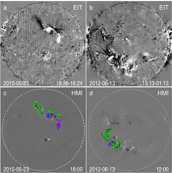
Figure 3.: Top: bright post-eruption arcades and dark dimmings in SOHO/EIT 195 Å difference images for eruptions 1A (2010 May 23, panel a) and 15B (2012 June 13, panel b). Bottom: corresponding SDO/HMI pre-event magnetograms (panels c and d) overlaid with contours of extracted dimmings (dark green for AIA and light green for EIT) and arcades (blue for AIA and pink for EIT). The contours illustrate the acceptable correspondence between the areas selected from the images produced by the two instruments.F-contours

All of these comparisons provide a basis for a general conclusion that with the adopted criteria, our procedures extract in the SDO/AIA 193 Å images the same dimmings and arcades as in the SOHO/EIT 195 Å images and AIA data can be used instead of EIT.

4 Comparison of Erupted Magnetic Fluxes

The second procedure, which should be considered, is the comparison of the erupted magnetic fluxes as measured by the SOHO/MDI and SDO/HMI magnetographs. In the period between the beginning of HMI observations in 2010 May and end of MDI observations in 2011 April, there were no large eruptions in ARs. Moreover, many of the Group A events considered in the preceding section were associated with filament eruptions outside ARs and had very small magnetic fluxes. It is not reasonable to compare the MDI and HMI fluxes of these eruptions. Instead, we will compare the total magnetic fluxes of the 34 largest ARs, which were observed near the solar disk center during the concurrent MDI and HMI observations and had the sunspot area greater than 100 millionths of the Sun visible hemisphere ($\mu$Hem) (see, e.g., the Solar Monitor site https://www.solarmonitor.org). Although the measurements with HMI and MDI have been compared previously, e.g. by Liu et al. (2012), we are not aware of such comparisons for magnetic fluxes erupted from large, developed active regions, where magnetic fields are strong and saturation-like distortions are probable.

The observation date, time, NOAA number, coordinates, and maximum areas of these ARs are listed in Table T-Table2. For each of these ARs, using data from both magnetographs, we calculated the total unsigned magnetic flux from the line-of-sight photospheric field within a single topologically-connected area, where the magnetic field strength exceeded 10 % of the maximum value over the entire magnetogram, but was not less than 15 G. All full-disk magnetograms were reduced to the $512\times 512$ pixels format. For MDI we used level 1.8 magnetograms recalibrated in 2008 December. The corresponding MDI and HMI FITS files were downloaded from the Stanford University sites of the MDI Daily Magnetic Field Synoptic Data (http://soi.stanford.edu/magnetic/index5.html) and from the Stanford Joint Science Operations Center (http://jsoc2.stanford.edu/data/hmi/fits/).

Table 2.: The SOHO/MDI and SDO/HMI magnetic fluxes of the largest ARs over the period from 2010 May to 2011 April.T-Table2

Date	Time	AR	Position	Area	Magnetic flux
	hh, UT	number		[$\mu$Hem]	[$10^{20}$ Mx]
					$\Phi_{\mathrm{MDI}}$	$\Phi_{\mathrm{HMI}}$
2010-05-24	08	11072	S15W23	130	94	63
2010-06-04	08	11076	S27W42	190	72	51
2010-07-04	08	11084	S19W33	150	35	27
2010-07-13	08	11087	N12E16	130	256	169
2010-07-22	08	11089	S24E32	310	144	114
2010-08-02	00	11092	N13E07	290	109	70
2010-08-07	08	11093	N12E31	180	72	54
2010-08-30	08	11101	N12W07	140	66	46
2010-09-17	08	11106	S20W09	110	229	161
2010-09-20	08	11108	S30E22	420	142	115
2010-09-28	08	11109	N22W12	420	248	173
2010-10-17	08	11112	S18W42	120	120	85
2010-10-18	08	11113	N18E09	160	47	34
2010-10-20	08	11115	S29W01	190	48	30
2010-10-28	00	11117	N22W42	450	237	165
2010-11-02	08	11120	N39E28	120	51	37
2010-11-16	08	11124	N14W44	260	137	101
2010-12-01	08	11130	N12W41	190	130	95
2010-12-08	08	11131	N31W11	430	166	126
2010-12-09	08	11133	N14E04	120	160	130
2011-01-02	08	11141	N35W38	100	39	28
2011-01-05	08	11140	N34E01	210	108	55
2011-02-16	08	11158	S21W41	600	267	187
2011-02-19	08	11162	N18W20	260	299	209
2011-02-21	08	11161	N11W42	260	199	137
2011-02-27	08	11163	N18E32	110	59	28
2011-03-05	08	11164	N25W33	570	367	267
2011-03-11	16	11166	N09W40	750	344	247
2011-03-13	08	11169	N19W36	260	196	135
2011-03-24	16	11176	S15E44	490	200	155
2011-03-27	08	11178	S15E29	130	50	38
2011-03-31	11	11183	N15E13	330	194	135
2011-04-05	16	11184	N17W27	170	138	95
2011-04-06	16	11185	N23E36	100	37	28

The relationship between the MDI, $\Phi_{\mathrm{MDI}}$, and HMI, $\Phi_{\mathrm{HMI}}$, AR magnetic fluxes calculated in this way is shown in Figure F-magflux. Its best linear fit in a wide range of the flux values of $\Phi_{\mathrm{MDI}}\simeq 35-350$ and $\Phi_{\mathrm{HMI}}\simeq 30-270$ (in $10^{20}$ Mx units) is $\Phi_{\mathrm{MDI}}=(3.1\pm 3.5)+(1.38\pm 0.03)\Phi_{\mathrm{HMI}}$ with a correlation coefficient of $r\approx 0.99$. Within the measurement errors, the factor we obtained from the analysis of the magnetic flux of ARs is consistent with the result of Liu et al. (2012), who established by a pixel-by-pixel comparison that the line-of-sight pixel-averaged magnetic signal inferred from MDI magnetograms was greater than that derived from the HMI data by the same scaling factor of 1.4. A close factor of 1.35 was also found by Svalgaard and Sun (2016). The differences between the measurements from MDI and HMI data can be due to their different calibration and a number of other factors (see Riley et al., 2014; Watson, Penn, and Livingston, 2014; Couvidat et al., 2016). Thus, in the transition from SOHO to SDO data, the relation $\Phi_{\mathrm{MDI}}=1.4\Phi_{\mathrm{HMI}}$ should be used.

Figure 4.: Relationship between the MDI and HMI magnetic fluxes of the largest ARs over the period from 2010 May to 2011 April (see Table T-Table2). The dotted line corresponds to $\Phi_{\mathrm{MDI}}=1.4\Phi_{\mathrm{HMI}}$.F-magflux

5 Transition Procedure

The results of the two previous sections allow us to adapt the SOHO diagnostic tool presented in Articles I and II to SDO data and current measurements. The updated tool does not need SOHO data. For the extraction of dimming and arcade areas for a particular eruption, it is sufficient to apply the cross-calibration factor between the EIT 195 Å and AIA 193 Å images. It is possible to simply adopt CCF $\approx 5$ for $\tau_{\mathrm{exp}}\approx 2.0$ or CCF $\approx 7$ for $\tau_{\mathrm{exp}}\approx 2.9$, based on Figure F-CCfactor for the first years. After that, one should download a FITS file of the HMI magnetogram that precedes the onset of an eruption and a number of AIA files covering approximately the duration of an associated soft X-ray flare. By analogy with the SOHO diagnosis, for the extraction of the SDO dimmings and arcades it is sufficient to take the AIA files with a 12-min interval. All AIA images should be corrected to a single pre-event exposure time (2.0 or 2.9 s) and divided by the CCF before the extraction of the arcade and dimming areas. Then, by coaligning the extracted areas with the HMI magnetogram, the corresponding erupted flux, $\Phi_{\mathrm{HMI}}$, is calculated.

Possible magnitudes as well as the onset and peak times of a geomagnetic storm and Forbush decrease are estimated by means of conversion of the corresponding empirical expressions, obtained in Articles I and II for SOHO data, in accordance with a relation $\Phi_{\mathrm{MDI}}=1.4\Phi_{\mathrm{HMI}}$. For SDO data, these expressions are as follows (again $\Phi_{\mathrm{HMI}}$ is in units of $10^{20}$ Mx):

• GMS intensity (Dst and Ap indexes)

  $$\mathrm{Dst\ [nT]}=30-15.4(\Phi_{\mathrm{HMI}}+3.8)^{1/2},$$

  $$\mathrm{Ap\ [2nT]}=1.12\Phi_{\mathrm{HMI}}.$$

• FD magnitude

  $$A_{\mathrm{F}}\ [\%]=-0.3+0.042\Phi_{\mathrm{HMI}}.$$

• The onset ($\Delta T_{\mathrm{o}}$) and peak ($\Delta T_{\mathrm{p}}$) transit times, i.e. the intervals between the eruption time (maximum time of an associated soft X-ray burst) and the start and peak of a corresponding GMS

  $$\Delta T_{\mathrm{o}}\ [\mathrm{h}]=98/(1+0.00616\Phi_{\mathrm{HMI}}),$$

  $$\Delta T_{\mathrm{p}}\ [\mathrm{h}]=118/(1+0.0056\Phi_{\mathrm{HMI}}).$$

6 Examples

Now we consider some examples of an SDO-based post-diagnosis related to several large eruptions in ARs located not far from the solar disk center and to major GMSs, which occurred during the current Solar Cycle 24. As already noted, due to a relatively low level of solar activity after 2009, only few major GMSs with Dst $<-100$ nT occurred. Most of the GMSs were caused by filament eruptions outside ARs and sometimes by high-speed solar wind from coronal holes (Gopalswamy et al., 2015; Gopalswamy, Tsurutani, and Yan, 2015). For instance, the strongest geomagnetic storm of the current solar cycle with a minimum Dst $=-228$ nT on 2015 March 17 was initiated by a large south-west filament eruption near AR 12297. Note that, according to our estimations, its erupted magnetic flux, $\Phi_{\mathrm{HMI}}\approx 90.5\times 10^{20}$ Mx (corresponding to the flux measured by MDI of $\Phi_{\mathrm{MDI}}\approx 126.7\times 10^{20}$ Mx), was larger than the fluxes in filament eruptions, which caused the GMS during Solar Cycle 23 (blue triangles in Figure 4 of Article I).

Table T-Table3 presents the results of the SDO-based diagnosis of five flare-associated eruptions in ARs carried out according to the procedure described in the previous section. The table lists parameters of a solar event in the second to sixth columns, including the date, peak time, coordinates, and GOES class of a related flare (second to fifth columns), and a total unsigned magnetic flux calculated from HMI magnetograms in dimmings and arcades in the sixth column. The seventh to nineteenth columns are related to the geospace disturbance, including its peak date and time, and estimated (letter code “est”) and observed (“obs”) parameters of a corresponding GMS and FD. Information on the observed hourly Dst index was taken from the WDC2 Kyoto service (http://wdc.kugi.kyoto-u.ac.jp/dstdir/index.html), while the values of the three-hour Ap index were estimated in the GeoForschungsZentrum (GFZ), Potsdam (ftp://ftp.gfz-potsdam.de/pub/home/obs/kp-ap/wdc/). The onset transit time, $\Delta T_{\mathrm{o}}$, is defined as an arrival time of the corresponding interplanetary disturbance (shock wave) at Earth indicated by the geomagnetic storm sudden commencement (SSC) (http://www.obsebre.es/en/rapid). Following Article I, the FD maximum magnitude is adopted; this magnitude corresponds to a cosmic ray rigidity of 10 GV evaluated from data of the world network of neutron monitors using the global survey method (Krymskii et al., 1981; Belov et al., 2005). Additionally, the eighteenth and nineteenth columns of Table T-Table3 list the hourly strength of the total interplanetary magnetic field near the Earth, $Bt$, and its $Bz$ component according to the Operating Missions as a Node on the Internet (OMNI) data (ftp://spdf.gsfc.nasa.gov/pub/data/omni/low˙res˙omni/).

Table 3.: Results of the SDO-based post-diagnosis of some eruptions of Solar Cycle 24.T-Table3

No	Eruption					Geomagnetic storm									Forbush		Magnetic
															decrease		field [nT]
	Date	Time	Position	Flare	$\Phi_{\mathrm{HMI}}$	Peak	Dst [nT]		Ap [2nT]		$\Delta T_{\mathrm{o}}$ [h]		$\Delta T_{\mathrm{p}}$ [h]		[%]		$Bt$	$Bz$
		UT		class	[$10^{20}$ Mx]	dd/hh	est	obs	est	obs	est	obs	est	obs	est	obs
1	2012-03-07	00:24	N17E27	X5.4	178.5	09/09	-178	-131	200	132	47	35	59	56	7.2	11.7	23.1	-16.1
2	2012-07-12	16:49	S15W01	X1.4	197	15/19	-188	-127	220	132	44	49	56	65	8.0	6.4	27.3	-17.7
3	2013-03-15	06:58	N11E12	M1.1	85.5	17/21	-116	-132	96	111	64	47	80	62	3.3	4.6	17.8	-14
4	2015-06-21	02:06	N12E13	M2.6	234.4	23/05	-208	-204	263	236	40	40	51	52	9.5	8.4	37.7	-26.3
5	2015-12-28	12:45	N19W22	M1.8	128.3	01/01	-147	-117	144	80	55	63	69	84	5.1	4.3The observed FD magnitude was evaluated from data of two high-latitude different-hemisphere stations, Thule and McMurdo.	16.9	-15.8

Table T-Table3 confirms the results of Articles I and II that the early diagnosis of the eruptions, based on the erupted magnetic flux evaluated in this case from SDO data, provides an approximate assessment for the importance of the related space weather disturbances. Particularly, the estimated values of Dst, Ap, $\Delta T_{\mathrm{o}}$, $\Delta T_{\mathrm{p}}$, and FD are comparable with the observed ones. According to the NOAA space weather scale (http://www.swpc.noaa.gov/noaa-scales-explanation), four events (Nos. 1 – 3 and 5) are classified as G2 – G3 (moderate – strong) storms, and one (No. 4) as G4 (severe) storm, judging from both the estimated and observed GMS intensity.

Table T-Table3 presents an apparent scattered correspondence between the estimated and observed parameters of the GMSs and FDs. Indeed, the larger the erupted flux, the stronger the actual intensity of the GMSs and FDs, and shorter the time intervals between the parent eruption and the GMS onset and peak are. For example, the Pearson correlation coefficient between the estimated Dst and its observed value is 0.61. On average, $\mathrm{Dst}_{\mathrm{obs}}/\mathrm{Dst}_{\mathrm{est}}=0.87\pm 0.19$ ($\pm 22\%$), while the role of the $Bz$ component seems to be comparable, $-Bz/Bt=0.75\pm 0.11$ ($\pm 15\%$). Thus, the differences between the estimated and observed Dst can be mostly due to the unaccounted $Bz$. There is also a close correspondence with a correlation coefficient of 0.91 between the erupted flux (sixth column) and the total magnetic field strength ($Bt$ in the eighteenth column) brought to Earth by the ICMEs.

The event on 2016 June 21 (No. 4 in Table T-Table3) with the largest erupted flux resulted in the most intense GMS and FD, having also the shortest transit times and strongest interplanetary magnetic field. In some events, for example Nos. 1 and 2, the estimated GMS intensity, measured both by the Dst and Ap indexes, markedly exceeds the observed one, while the magnitudes of the FDs are much closer. This is apparently due to the fact that in these cases the negative $Bz$ component, which determines the GMS intensity, but not considered in our preliminary tool, amounts to only part of the total interplanetary magnetic strength, which determines the FD magnitude.

As for the temporal parameters of GMSs, a close correspondence between the estimated and observed values of both $\Delta T_{\mathrm{o}}$ and $\Delta T_{\mathrm{p}}$ is present for event No. 4. In other cases, some differences can be seen. Our simple tentative estimates have been done as if they were issued right after an eruption, without taking into account preceding activity, actual magnetic field and plasma distributions in the corona, ICME drag in the solar wind, and other factors.

7 Concluding Remarks

We compared quantitative parameters of CME-associated post-eruption arcades and dimmings observed with EUV telescopes and magnetographs aboard the SOHO and SDO spacecraft. Two basic facts have been established. First, with the adopted thresholds of relative brightness changes, practically the same arcade and dimming areas are extracted from EIT 195 Å and AIA 193 Å images, if their cross-calibration factor in a range of 3.6 – 5.8 and 5.0 – 8.2 is taken into account for the AIA exposure time 2.0 and 2.9 s, respectively. Second, for the same photospheric areas of strong magnetic fields in large active regions, the MDI line-of-sight magnetic flux systematically exceeds the HMI flux by a factor of 1.4.

These results allowed us to upgrade the tool for the early diagnostics of AR eruptions described in Articles I and II for SOHO data to the current SDO observations. Empirical relationships are obtained to connect the erupted magnetic flux measured from SDO data with possible intensity and temporal parameters of forthcoming non-recurrent GMSs and FDs. The case studies presented here confirm that the updated diagnostic tool based on SDO data also produces acceptable results, providing a prompt and sufficiently correct assessment of the importance of forthcoming space weather disturbances using only magnetic flux within the arcade and dimming areas. The tool presented here and previously in Articles I and II corroborates the idea that parameters of solar eruptions, CMEs and ICMEs, and geospace disturbances are largely determined not only by the characteristics of associated ARs and flares, but by a measurable quantity as this erupted magnetic flux in arcades and dimmings (see Article I; Démoulin, 2008; Mandrini et al., 2009 for a review).

It is clear, however, that the proposed tool for the early preliminary prognostic estimations does not take into account many factors affecting the GMS and FD characteristics. Consequently, as in Articles I and II, we do not pursue exact estimates of the parameters of GMSs and FDs and focus instead on their possible importance. In practice, our tool should be the starting point of a complex of comprehensive forecasting tools, which would consider information on near-the-Sun CMEs, various models of eruptions and drag of ICMEs propagating in the solar wind, stereoscopic observations, estimation of a probable sign of the $Bz$ component, and others (see, e.g., Gopalswamy, Tsurutani, and Yan, 2015, and references therein).

Acknowledgments

We appreciate the painstaking work of the anonymous reviewer for valuable remarks and recommendations that significantly helped us to bring this article to its final form. The authors thank the SOHO/EIT and MDI and SDO/AIA and HMI teams for their open data used in our study. SOHO is a project of international cooperation between ESA and NASA. SDO is a mission of the NASA’s Living With a Star (LWS) Program. We are grateful to A.V. Belov for his assistance and useful discussions. This research was partially supported by the Russian Foundation of Basic Research under grant 14-02-00367.

Disclosure of Potential Conflicts of Interest

The authors claim that they have no conflicts of interest.

References

- Belov (2009) Belov, A.V.: 2009, Proc. IAU Symp. 257, 439. DOI
- Belov et al. (2005) Belov, A., Baisultanova, L., Eroshenko, E., Mavromichalaki, H., Yanke, V., Pchelkin, V., et al.: 2005, J. Geophys. Res. 110, A09S20. DOI
- Bothmer and Zhukov (2007) Bothmer, V., Zhukov, A.: 2007, In: Bothmer, V. and Daglis, I.A. (eds.) Space Weather - Physics and Effects, 31. DOI
- Cane (2000) Cane, H.V.: 2000, Space Sci. Rev. 93, 55. DOI
- Chertok and Grechnev (2005) Chertok, I.M., Grechnev, V.V.: 2005, Sol. Phys. 229, 95. DOI
- Chertok et al. (2013) Chertok, I.M., Grechnev, V.V., Belov, A.V., Abunin, A.A.: 2013, Sol. Phys. 282, 175 (Article I). DOI
- Chertok et al. (2015) Chertok, I.M., Abunina, M.A., Abunin, A.A., Belov, A.V., Grechnev, V.V.: 2015, Sol. Phys. 290, 627 (Article II). DOI
- Couvidat et al. (2016) Couvidat, S., Schou, J., Hoeksema, J.T., Bogart, R.S., Bush, R.I., Duvall, T.L.: 2016, Sol. Phys. 291, 1887. DOI
- Démoulin (2008) Démoulin, P.: 2008, Ann. Geophys. 26, 3113. DOI
- Delaboudinière et al. (1995) Delaboudinière, J.-P., Artzner, G.E., Brunaud, J., Gabriel, A.H., Hochedez, J.F., Millier, F., et al.: 1995, Sol. Phys. 162, 291. DOI
- Domingo, Fleck, and Poland (1995) Domingo, V., Fleck, B., Poland, A.I.: 1995, Sol. Phys. 162, 1. DOI
- Gopalswamy, Tsurutani, and Yan (2015) Gopalswamy, N., Tsurutani, B., Yan, Y.: 2015, Progress in Earth and Planetary Science, 2, 13. DOI
- Gopalswamy et al. (2015) Gopalswamy, N., Yashiro, S., Xie, H., Akiyama, S., Mäkelä, P.: 2015, J. Geophys. Res. 120, 9221. DOI
- Gosling (1993) Gosling, J.T.: 1993, J. Geophys. Res. 113, 18937. DOI
- Grechnev et al. (2003) Grechnev, V.V., Lesovoi, S.V., Smolkov, G.Y., Krissinel, B.B., Zandanov, V.G., Altyntsev, A.T., Kardapolova, N.N., Sergeev, R.Y., Uralov, A.M., Maksimov, V.P., Lubyshev, B.I.: 2003, Sol. Phys. 216, 239. DOI
- Hanaoka et al. (1994) Hanaoka, Y., Shibasaki, K., Nishio, M., Enome, S., Nakajima, H., Takano, T., Torii, C., Sekiguchi, H., Bushimata, T., Kawashima, S., Shinohara, N., Irimajiri, Y., Koshiishi, H., Kosugi, T., Shiomi, Y., Sawa, M., Kai, K.: 1994, Proc. Kofu Symp., 35.
- Harra et al. (2011) Harra, L.K., Mandrini, C.H., Dasso, S., Gulisano, A.M., Steed, K., Imada, S., et al.: 2011, Sol. Phys. 268, 213. DOI
- Hudson and Cliver (2001) Hudson, H.S., Cliver, E.W.: 2001, J. Geophys. Res. 106, 25199. DOI
- Kahler (1977) Kahler, S.: 1977, ApJ 214, 891. DOI
- Kochanov et al. (2013) Kochanov, A.A., Anfinogentov, S.A., Prosovetsky, D.V., Rudenko, G.V., Grechnev, V.V.: 2013, PASJ 65. DOI
- Krymskii et al. (1981) Krymskii, G.F., Kuz’min, A.I., Krivoshapkin, P.A., Samsonov, I.S., Skripin, G.V., Transkij, I.A., Chirkov, N.P.: 1981, Kosmicheskie luchi i solnechnyi veter (Cosmic Rays and Solar Wind), Novosibirsk: Nauka.
- Lemen et al. (2012) Lemen, J.R., Title, A.M., Akin, D.J., Boerner, P.F., Chou, C., Drake, J.F., et al.: 2012, Sol. Phys. 275, 17. DOI
- Liu et al. (2012) Liu, Y., Hoeksema, J.T., Scherrer, P.H., Schou, J., Couvida, C., Bush, T.L., et al.: 2012, Sol. Phys. 279, 295. DOI
- Mandrini et al. (2009) Mandrini, C.H., Nakwacki, M.S., Attrill, G., van Driel-Gesztelyi, L., Dasso, S., Démoulin, P.: 2009, In: Gopalswamy, N., Webb, D.F. (eds.), Universal Heliospheric Processes, IAU Symp. 257, 265. DOI
- Miklenic, Veronig, and Vršnak (2009) Miklenic, C.H., Veronig, A.M., Vršnak, B.: 2009, A&A 499, 893. DOI
- Pesnell, Thompson, and Chamberlin (2012) Pesnell, W. D., Thompson, B.J., Chamberlin, P.C.: 2012, Sol. Phys. 275, 3. DOI
- Qiu et al. (2007) Qiu, J., Hu, Q., Howard, T.A., Yurchyshyn, V.B.: 2007, ApJ 659, 758. DOI
- Reinard and Biesecker (2008) Reinard, A.A., Biesecker, D.A.: 2008, ApJ 674, 576. DOI
- Reinard and Biesecker (2009) Reinard, A.A., Biesecker, D.A.: 2009, ApJ 705, 914. DOI
- Richardson and Cane (2011) Richardson, I.G., Cane, H.V.: 2011, Sol. Phys. 270, 609. DOI
- Riley et al. (2014) Riley, P., Ben-Nun, M., Linker, J.A., Mikic, Z., Svalgaard, L., Harvey, J., et al. R.: 2014, Sol. Phys. 289, 769. DOI
- Scherrer et al. (1995) Scherrer, P.H., Bogart, R.S., Bush, R.I., Hoeksema, J.T., Kosovichev, A.G., Schou, J., et al.: 1995, Sol. Phys. 162, 129. DOI
- Scherrer et al. (2012) Scherrer, P.H., Schou, J., Bush, R.I., Kosovichev, A. G., Bogart, R. S., Hoeksema, J. T, et al.: 2012, Sol. Phys. 275, 207. DOI: 10.1007/s11207-011-9834-2
- Sterling et al. (2000) Sterling, A.C., Hudson, H.S., Thompson, B.J., Zarro, D.: 2000, ApJ 532, 628. DOI
- Svalgaard and Sun (2016) Svalgaard, L., Sun, X.: 2016, http://hmi.stanford.edu/hminuggets/?p=1510.
- Thompson et al. (1998) Thompson, B.J., Plunkett, S.P., Gurman, J.B., Newmark, J.S., St. Cyr, O.C., Michels, D.J.: 1998, Geophys. Res. Lett. 25, 2465. DOI
- Tripathi, Bothmer, and Cremades (2004) Tripathi, D., Bothmer, V., Cremades, H.: 2004, A&A 422, 337. DOI
- Uralov et al. (2014) Uralov, A.M., Grechnev, V.V., Rudenko, G.V., Myshyakov, I.I., Chertok, I.M., Filippov, B.P., Slemzin, V.A.: 2014, Sol. Phys. 289, 3747. DOI
- Watson, Penn, and Livingston (2014) Watson, F.T., Penn, M.J., Livingston, W.: 2014, ApJ 787, 22. DOI
- Yashiro et al. (2013) Yashiro, S., Gopalswamy, N., Mäkelä, P., Akiyama, S.: 2013, Sol. Phys. 284, 5. DOI