Polynomial Time Efficient Construction Heuristics for Vertex Separation Minimization Problem

Abstract

Vertex Separation Minimization Problem (VSMP) consists of finding a layout of a graph $G=(V,E)$ which minimizes the maximum vertex cut or separation of a layout. It is an NP-complete problem in general for which metaheuristic techniques can be applied to find near optimal solution. VSMP has applications in VLSI design, graph drawing and computer language compiler design. VSMP is polynomially solvable for grids, trees, permutation graphs and cographs. Construction heuristics play a very important role in the metaheuristic techniques as they are responsible for generating initial solutions which lead to fast convergence. In this paper, we have proposed three construction heuristics H1, H2 and H3 and performed experiments on Grids, Small graphs, Trees and Harwell Boeing graphs, totaling 248 instances of graphs. Experiments reveal that H1, H2 and H3 are able to achieve best results for 88.71%, 43.5% and 37.1% of the total instances respectively while the best construction heuristic in the literature achieves the best solution for 39.9% of the total instances. We have also compared the results with the state-of-the-art metaheuristic GVNS and observed that the proposed construction heuristics improves the results for some of the input instances. It was found that GVNS obtained best results for 82.9% instances of all input instances and the heuristic H1 obtained best results for 82.3% of all input instances.

1 Introduction

Graph layout problems are a class of combinatorial optimization problems whose goal is to find a layout of an input graph G to optimize a certain objective function. A linear layout or layout of an undirected graph $G=(V,E)$, where $|V|=n$ is the bijective function $\varphi\colon V\rightarrow[n]=\{1,2,\dots,\emph{n}\}$. Set of all layouts is denoted by $\Phi(G)$. A Region in layout is defined as the area between two consecutive vertices in the layout. Vertex Separation minimization problem (VSMP) is to find a layout $\varphi^{*}\in\Phi(G)$ of a graph $G=(V,E)$ which minimizes the vertex separation (VS) where $VS=\max_{i\in[|V|]}⁡\delta(i,\varphi,G)$ for a layout $\varphi$ where, $\delta(i,\varphi,G)=|{u\in L(i,\varphi,G)\colon\exists v\in R(i,\varphi,G)\wedge(u,v)\in E(G)}|$, $L(i,\varphi,G)=\{u\in V\colon\varphi(u)\leq i\}$ and $R(i,\varphi,G)=\{u\in V\colon\varphi(u)>i\}$ [1, 4]. VSMP is NP-complete in general and has applications in VLSI design, graph drawing and computer language compiler design [2].

Further, in this paper, a vertex identifier corresponds to the vertices of graphs which are assumed to be the natural numbers 1,…,n. For a vertex $u\in V(G)$, neighbourhood of u in G, $N(u)=\{v\in V(G)\colon(u,v)\in E(G)\}$ and degree of u in G, $d_{G}(u)=|{v\in V(G)\colon(u,v)\in E(G)}|$. Fig. 1(b) represents a linear layout of Fig. 1(a). VS for this layout $\varphi$ of G is 3.

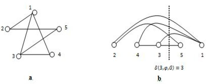
Figure 1: (a) A graph and (b) layout $\varphi=(2,4,3,5,1)$

VSMP is polynomially solvable for grids, trees, permutation graphs and cographs [1, 4]. This problem has been explored using metaheuristics namely, variable neighbourhood search by [2, 5] in which they have proposed construction heuristics to generate an initial solution. Noberto et al. [3] highlight the importance of construction heuristics in metaheuristics. They have proposed eight construction heuristics and have compared all the construction heuristics. In this paper, we have proposed three construction heuristics H1, H2, H3. An experiment has been performed to compare all the construction heuristics on the test instances of Grids, Small graphs, Trees and Harwell Boeing graphs, totaling 248 instances of graphs. Experiments reveal that H1, H2 and H3 are able to achieve best results for 87.9%, 43.5% and 37.1% of the total instances respectively, while the best construction heuristic in the literature achieves the best solution for 39.9% of the total instances. We have also compared the results of H1 with the state-of-the-art metaheuristic general variable neighbourhood search (GVNS) [5] and observed that the proposed construction heuristics improves the results for some of the input instances. It was also observed that GVNS obtains best results for 82.9% instances of all input instances while the heuristic H1 obtained best results for 82.3% instances of all input instances. Further, in this paper Section 2 presents the construction heuristics proposed in this paper followed by computational experiments to show the efficiency of heuristics in Section 3.

2 Construction Heuristics

In this section, three construction heuristics have been proposed. These heuristics construct a layout by iteratively adding vertices to an initially empty layout. In each iteration, heuristic H1 tries to place a vertex u in the partial layout which minimizes its contribution as well as the contribution of vertices which are already placed in the partial layout. Motivation behind H2 and H3 is that if adjacent vertices are closely placed then they contribute to fewer regions. Further, in order to minimize the number of regions to which a vertex contributes, vertices of smaller degree are placed first in the partial layout. In the following sections, we describe the three construction heuristics which are essentially greedy methods.

2.1 Heuristic H1

This procedure is outlined in Algorithm 1. Let layout be the (partial) layout under construction. The set unvisited is the set of vertices of graph G which are not in layout.

The time complexity of H1 is $O(n^{2}\cdot\Delta(G))$.

Step 1:

$unvisited=\{1,\dots,n\}$

Step 2:

Select a vertex $v\in unvisited$ such that $d_{G}(v)$ is least

Step 3:

$layout=(v)$

Step 4:

$unvisited=unvisited\setminus\{v\}$

Step 5:

while $|layout|\neq n$

Step 6:

$S=\{v\in layout\colon v$ is adjacent to least number of vertices in $unvisited$}

Step 7:

$P=\{w\in unvisited\colon w$ is adjacent to largest number of vertices in $S$}

Step 8:

$Q=\{u\in P\colon u$ is adjacent to least number of vertices in $unvisited$}

Step 9:

Select $v\in Q$ randomly

Step 10:

$layout=(layout,v)$

Step 11:

$unvisited=unvisited\setminus\{v\}$

Step 12:

endwhile

Figure 2: Algorithm1: Heuristic H1

2.2 Heuristic H2

Algorithm 2 presents heuristic H2. Time complexity of Heuristic H2 is $O(n^{2}\cdot\log n)$.

Step 1:

u = minimium degree vertex of a graph G

Step 2:

$unvisited=V\setminus\{u\}$

Step 3:

$layout=(u)$

Step 4:

S = sort N(u) in ascending order of the degrees

Step 5:

$layout=(layout,S)$

Step 6:

$unvisited=unvisited\setminus S$

Step 7:

while $|layout|\neq|V(G)|$

Step 8:

$degree=\{degree_{w}=|N(w)\setminus layout|\colon w\in V(G)\}$

Step 9:

select a vertex v such that $degree_{v}$ is least but non-zero

Step 10:

if $v\notin layout$

Step 11:

$layout=(layout,v)$

Step 12:

$unvisited=unvisited\setminus{v}$

Step 13:

endif

Step 14:

$S=N(v)\setminus layout$

Step 15:

$S^{\prime}$ = sort $S$ according to their values in degree in ascending order

Step 16:

$layout=(layout,S^{\prime})$

Step 17:

$unvisited=unvisited\setminus S^{\prime}$

Figure 3: Algorithm2: Heuristic H2

2.3 Heuristic H3

This Heuristic is similar to H2, but as opposed to the selection in Step 9 of Heuristic H2, preference is given to a vertex v in the partially constructed layout with least $\varphi(\emph{v})$. Time complexity of H3 is same as H2.

3 Computational Experiments

In this section we present the computational experiments that were performed to test the effectiveness of the proposed construction heuristics. The code was implemented in Matlab 7.0 and all the experiments were conducted on an Intel i3 based system with 4 GB RAM. The experiment to compare the construction heuristics was performed on the four sets of instances previously used for this problem [3]. The test set includes Small, Harwell-Boeing (HB) graphs, Grids and Trees. Since GVNS was tested on Harwell-Boeing (HB) graphs, Grids and Trees in the literature, therefore, construction heuristic H1 and GVNS are compared on these instances only. The order of graph ranges from 9 to 2916. For each heuristic H1, H2 and H3, 30 runs were carried out and the best value of vertex separation was recorded.

3.1 Comparison between Construction Heuristics

In this section the proposed construction heuristics are compared with those available in the literature. Random represents randomly generated solution. C1 and C2 are the construction heuristics proposed in [2] and HA1, HA2, HA3, HA4, HN1, HN2, HN3 and HN4 have been proposed in [3]. Heuristics H1, H2 and H3 have been presented in this paper. Table 1 presents the average vertex separation for different construction heuristics. The average vertex separation over all the instances are given in the last column ${}^{\prime}Average^{\prime}$. Results show that H1 outperforms all the heuristics. Table 2 presents number of best solution achieved using each heuristic. In the table, the last column ${}^{\prime}Sum^{\prime}$ represents the total number of instances for which heuristic achieves the best value. Number in bold indicates that the value is best in that column. Heuristic H1 achieves best result for 220 instances out of 248 instances which is equal to 88.71% of the total instances. Similarly, H2 and H3 achieve best results for 43.55% and 37.1% instances of total instances. Among the existing heuristics, a maximum of 39.92% of the total instances best solutions are obtained by HN1.

Table 1: Average vertex separation for different construction heuristics

Heuristics	Grid(52)	Small(84)	Tree(50)	HB(62)	Average
Random	553.08	9.26	43.6	229.03	185.15
C1	29.5	6.18	4.66	40.1	19.24
C2	28.5	5.01	11.08	34.7	18.58
HA1	38.19	4.32	5.24	53.65	23.94
HA2	684.35	12.21	61.7	294.58	233.71
HA3	38.5	4.26	5.22	53.08	23.84
HA4	688	11.68	61.68	294.15	234.19
HN1	28.5	4.05	7.66	49.23	21.2
HN2	687.94	6.76	12.86	235.45	207.99
HN3	30.44	4.14	7.52	51.27	22.12
HN4	697.96	6.51	13.36	233.52	209.63
H1	28.5	3.29	4.1	30.53	15.6
H2	28.52	4.02	15.74	35.48	19.45
H3	28.5	4.28	11.52	37.05	19.07

Table 2: Number of best solutions achieved for different construction heuristics

Heuristics	Grid(52)	Small(84)	Tree(50)	HB(62)	Sum
Random	0	0	0	1	1
C1	0	1	12	1	14
C2	52	7	6	8	73
HA1	0	20	0	4	27
HA2	0	0	0	1	1
HA3	0	23	4	4	33
HA4	0	0	0	1	1
HN1	52	29	12	6	99
HN2	0	1	1	1	3
HN3	1	27	14	3	45
HN4	1	0	0	1	2
H1	52	80	50	38	220
H2	51	31	3	23	108
H3	52	25	1	14	92

3.2 Comparison between H1 and GVNS

In this section, the best performing construction heuristic H1 is compared with the metaheuristic General Variable Neighbouhood Strategy (GVNS) [5]. Average vertex separation obtained by GVNS and H1 are listed in Table 3. Numbers in bold are the minimum in that column. Results show that for Trees, H1 performs better while performance of GVNS on HB instance is good. When the average is considered over all the instances, performance of GVNS and H1 is comparable. Table 4 presents the number of best solutions achieved using each heuristic. For grids, GVNS and H1 both are able to obtain optimal results. For trees, GVNS obtained optimal results for 40 instances out of 50 while H1 obtained optimal results for all the tree instances. In case of HB instances, GVNS obtained best results for 44 instances out of 62 while H1 was able to obtain optimal results for 33 instances only. When all the graphs are considered GVNS obtained best results in 136 cases out of 164 which is equal to 82.9% of all input instances while H1 obtained optimal results in 135 cases which is equal to 82.3% of all input instances.

Table 3: Average vertex separation for GVNS [5] and H1

Heuristics	Grid(52)	Tree(50)	HB(62)	Average
GVNS	28.5	4.3	24.6	19.85
H1	28.5	4.1	30.53	21.83

Table 4: Number of best solutions achieved using GVNS and H1

Heuristics	Grid(52)	Tree(50)	HB(62)	Sum
GVNS	52	40	44	136
H1	52	50	33	135

4 Conclusion

In this paper, we have proposed three polynomial time construction heuristics and compared with other construction heuristics. It was observed that these construction heuristics outperform other construction heuristics given in literature. The best performing construction heuristic H1 was also compared with the state-of-the-art metaheuristic GVNS. This construction heuristic achieves best results in larger number of cases than GVNS. Since a good initial population is expected to converge faster to a near optimal/optimal solution, therefore, initial solutions generated using this construction heuristic in any metaheuristic will lead to high quality solutions.

References

- [1] Diaz, J., J. Petit and M. Serna, A Survey of Graph Layout Problems, ACM Computing Surveys. 34 (2002), 313–356.
- [2] Duarte A., L. F. Escudero, R. Marti, N. Mladenovic, J. J. Pantrigo and J. Sanchez-Oro, Variable Neighborhood Search for the Vertex Separation Problem, Computers and Operations Research. 39 (2012), 3247–3255.
- [3] Garcia N. C., H. J. F. Huacuja, J. A. M. Flores, R. A. P. Rangel, J. J. G. Barbosa, J. M. C. Valadez, Comparative Study on Costructive Heuristics for the Vertex Separation Problem, Design of Intelligent Systems Based on Fuzzy Logic, Neural Networks and Nature-Inspired Optimization. (2015), 465–474.
- [4] Petit, J., Addenda to the Survey of Layout Problems, Bulletin of the EATCS. 105 (2011), 177–201.
- [5] Sanchez-Oro J., J. J. Pantrigo and A. Duarte, Combining intensification and diversification strategies in VNS. An application to the Vertex Separation Problem., Computers and Operations Research. 52 (2014), 209–219.