Non Fermi liquid behavior and continuously tunable resistivity exponents
in the Anderson-Hubbard model at finite temperature

Abstract

We employ a recently developed computational many-body technique to study for the first time the half-filled Anderson-Hubbard model at finite temperature and arbitrary correlation ($U$) and disorder ($V$) strengths. Interestingly, the narrow zero temperature metallic range induced by disorder from the Mott insulator expands with increasing temperature in a manner resembling a quantum critical point. Our study of the resistivity temperature scaling $T^{\alpha}$ for this metal reveals non Fermi liquid characteristics. Moreover, a continuous dependence of $\alpha$ on $U$ and $V$ from linear to nearly quadratic was observed. We argue that these exotic results arise from a systematic change with $U$ and $V$ of the “effective” disorder, a combination of quenched disorder and intrinsic localized spins.

A hallmark of a conventional Fermi liquid (FL) in good metals is the $T^{2}$ scaling of the resistivity ($\rho$) with temperature $T$. However, deviations from this behavior have been reported in several correlated electronic materials such as heavy fermions Gegenwart et al. (1998); Trovarelli et al. (2000); Julian et al. (1996); Coleman et al. (2001), rare earth nickelates Jaramillo et al. (2014), layered dichalcogenides Lahoud et al. (2014), and cuprates Damascelli et al. (2003); Hussey et al. (2003); Keimer et al. (2015). Various ideas for explaining non Fermi liquid (NFL) states have been proposed. For instance, a $T=0$ quantum critical point (QCP) could induce the linear $\rho\sim T$ scaling in the cuprates Anderson (2006); Keimer et al. (2015); Casey and Anderson (2011). In the NFL observed in the two-dimensional electron gas (2DEG) Bogdanovich and Popović (2002); Jaroszyński et al. (2002); Kravchenko and Sarachik (2004), charge or spin glassy metallic states could provide an alternative Arrachea et al. (2004); Dalidovich and Dobrosavljević (2002); Sachdev and Read (1996); Miranda and Dobrosavljević (2005). In spite of these important efforts, the understanding of NFLs in correlated systems still eludes theorists. Moreover, in heavy fermion experiments a puzzling continuous variation of the $\rho$ vs. $T$ scaling exponent $\alpha$ between 1 and 1.6 was found Gegenwart et al. (1998); Trovarelli et al. (2000); Julian et al. (1996); Coleman et al. (2001). Considering that the microscopic physics of the several NFL material families are quite different, it is a challenge to find a global understanding of NFL states in correlated systems. In particular, we need to identify concrete model Hamiltonian systems that not only support NFL states but also, within a single framework, capture various NFL systematics observed across different material families.

To address these issues, here we study the temperature characteristics of the unconventional metal known to develop at $T=0$ from the competition between strong electron interactions and disorder in the half-filled Anderson-Hubbard model on a square lattice. In the clean limit, the ground state is a Mott insulator (MI) and correlated metals arising from doping MI’s Deng et al. (2013) violate the $\rho\sim T^{2}$ scaling. In the other limit where quenched disorder dominates, single particle states are localized in two dimensions and these disorder-induced Anderson insulators often display variable range hopping behavior Imry (2002).

The surprising $T=0$ intermediate metallic state that results from the combination of correlations and disorder has been studied theoretically using Dynamical Mean Field Theory (DMFT) Dobrosavljevic et al. (2012); Song et al. (2008); Semmler et al. (2010); Tanasković et al. (2003); Aguiar et al. (2008), Quantum Monte Carlo Otsuka and Hatsugai (2000); Srinivasan et al. (2003); Chakraborty et al. (2007), Exact Diagonalization Kotlyar and Das Sarma (2001), and Hartree-Fock Heidarian and Trivedi (2004). Experimental results Kravchenko et al. (1995); Sarma et al. (1998); Nakatsuji et al. (2004); Sanchez-Palencia and Lewenstein (2010); Lahoud et al. (2014) are compatible with the zero temperature calculations. However, the finite temperature understanding of this exotic metal and its scaling is limited and several questions remain. How does a metal that arises from competing Mott and Anderson insulators behave at finite temperatures? What temperature scaling does the resistivity of the ensuing metal display? Is there a dependence of the exponent $\alpha$ on disorder and interaction strengths that can be tuned? Are spin or charge cluster states Miranda and Dobrosavljević (2005) responsible for such scaling behavior? Answers to these open questions are of relevance for experiments and theory alike.

In this publication, we study the half-filled Anderson-Hubbard model at finite temperature using the recently developed Mean Field-Monte Carlo (MF-MC) technique. This approach properly incorporates thermal fluctuations in a mean field theory mfm . Details and benchmarks are in Supplementary Material Sec. I. Using MF-MC, here we establish the disorder-interaction-temperature ($V-U-T$) phase diagram. In particular, we observed a disorder-induced continuous evolution from the Mott to the Anderson insulators with a strange metal in between. Our temperature analysis of this region unveils an intriguing quasi QCP behavior, with a narrow metallic region increasing in width with increasing temperature resembling a quantum phase transition. Through optical conductivity and resistivity calculations, we uncover a striking behavior: by changing $U$ and $V$, $\alpha$ can be tuned (akin to heavy fermions) from linear $\alpha=1$, as in cuprates, to near quadratic. Then disorder and interactions can be used to modify the scaling $\rho\sim T^{\alpha}$.

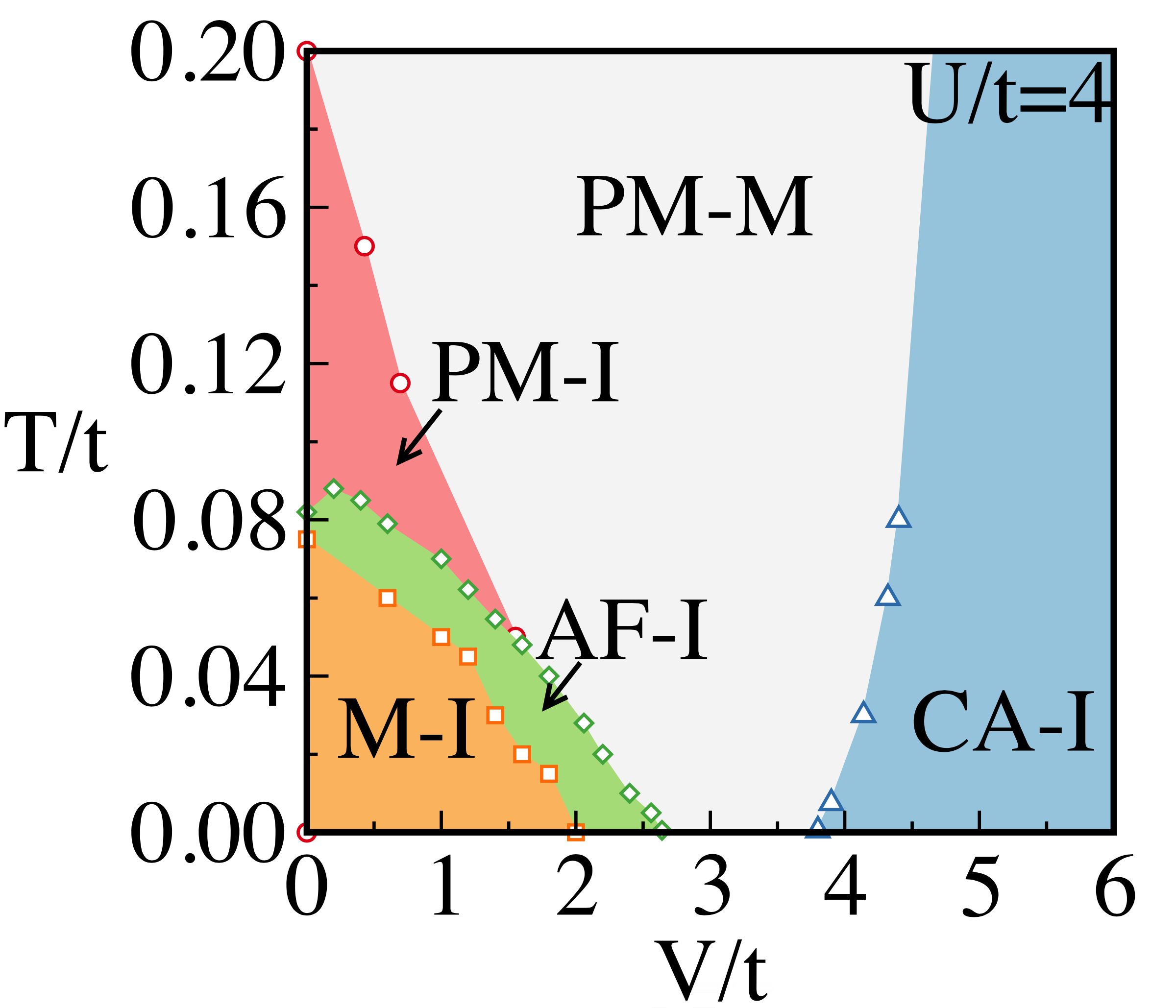
Figure 1: (color online) Temperature ($T$) vs. disorder ($V$) phase diagram at half filling for $U/t=4.0$ obtained using a $32^{2}$ square lattice. The zero temperature antiferromagnetic (AFM) Mott insulator (M-I) to gapless AFM insulator (AF-I) at $V\sim 2t$, and the subsequent transition to the paramagnetic metal (PM-M) at $V\sim 3t$, are both continuous within our accuracy. For $V>3.8t$ at $T=0$, we observe a disorder-induced correlated Anderson insulator (CA-I). Finally for $T/t\in[0.08,0.2]$ and small $V/t$, pink region, we find a gapless PM insulator (PM-I). Details are in the text.

The model is:

$$H=-t\sum_{\langle i,j\rangle\ \sigma}c^{\dagger}_{i,\sigma}c^{\phantom{\dagger}}_{i,\sigma}+\sum_{i}Un_{i\uparrow}n_{i\downarrow}+\sum_{i}(V_{i}-\mu)(n_{i\uparrow}+n_{i\downarrow}),$$

where the first term is the kinetic energy and the second the standard Hubbard repulsion. $c^{\phantom{\dagger}}_{i\sigma}$ ( $c^{\dagger}_{i\sigma}$) annihilates (creates) an electron at site $i$ with spin $\sigma$. The number operator is $n_{i\sigma}=c^{\dagger}_{i\sigma}c^{\phantom{\dagger}}_{i\sigma}$. The disorder $V_{i}$ at each site is chosen randomly in the interval $[-V,V]$ with uniform probability. The chemical potential $\mu$ is adjusted to achieve half filling globally. In MF-MC, we first Hubbard-Stratonovich decouple the interaction term, by introducing a vector auxiliary $\bm{m_{i}}$ and a scalar $\phi_{i}$ field at every site. The former couples to spin and latter to charge. Dropping the time dependence of the auxiliary fields (Aux. F.) a model with “spin fermion” characteristics arises. The Aux. F. are treated by classical MC that admits thermal fluctuations, and the fermionic sector is solved using Exact Diagonalization. Details of the considerable numerical effort involved are discussed in Supplementary Material Sec I.

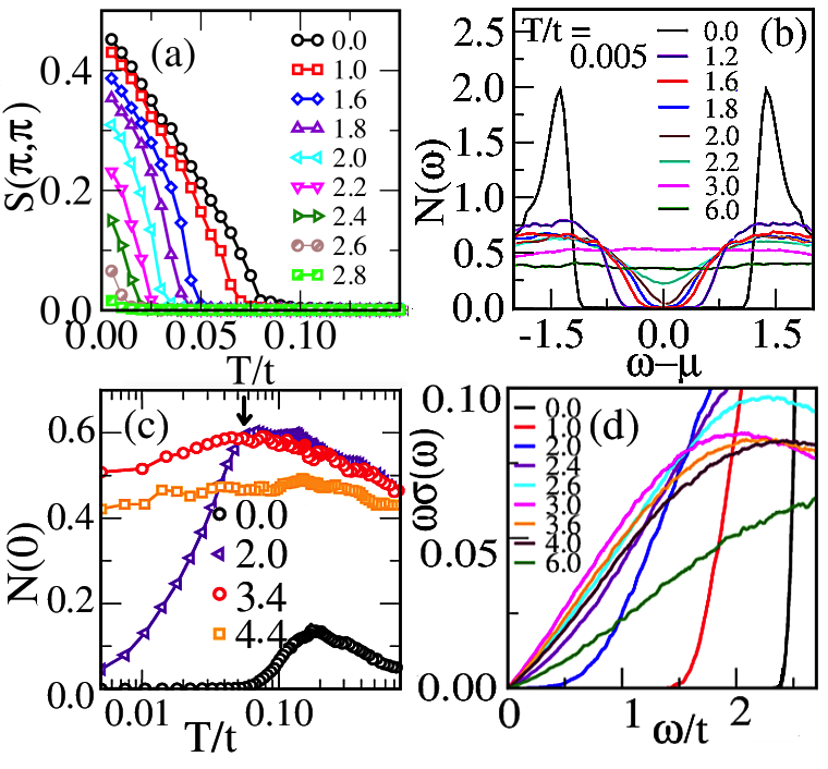
Figure 2: (color online) Examples of MF-MC data at $U/t=4$ used to construct the phase diagram Fig. 1. (a) Static magnetic structure factor at $\bm{q}=(\pi,\pi)$. Values of $V/t$ are in the column. (b) Low-$T$ density-of-states (DOS) $N(\omega)$ at various disorder strengths. (c) DOS $\omega=0$ weight at the four $V/t$’s indicated vs. $T/t$. Arrow indicates the maximum of $N(0)$ for $V/t=3.4$. (d) $\omega$ times the optical conductivity $\sigma(\omega)$, at $T/t=0.005$, for the several $V/t$’s indicated.

1. Phase diagram. Consider the phase diagram shown in Fig. 1 at the representative value $U/t=4$. Various indicators, such as the $(\pi,\pi)$ static magnetic structure factor, density of states (DOS), and optical conductivity $\sigma(\omega)$ were used (Fig. 2). At $T/t=0.005$ the antiferromagnetic (AFM) order is progressively reduced increasing $V/t$ as shown in Fig. 2 (a), and for $V\geq 2.6t$ the signal becomes negligible. At $V=0$, the magnetic order starts at $T/t=0.10$ upon cooling but the system remains insulating above this temperature, as expected, and a paramagnetic insulator (PM-I), is deduced based on the optical conductivity behavior discussed below. Increasing $V/t$, $T_{N}$ initially slightly increases and then reduces with increasing disorder upt . The metal insulator boundary decreases roughly linearly with $V/t$, collapsing to zero at $V/t=2.6$. Panel (b) shows the low-$T$ DOS, $N(\omega)$, for various disorder strengths. We find that the clean-limit Mott gap evolves into a pseudogap gap at $V/t\sim 2$. This pseudogap persists up to $V/t=2.8$ and flattens out for larger $V/t$, with the weight around $\omega=0$ decreasing gradually with disorder as the DOS spreads over a larger energy range due to increasing scattering. Thus, the AF-I, PM-M and CA-I phases in Fig. 1 are gapless.

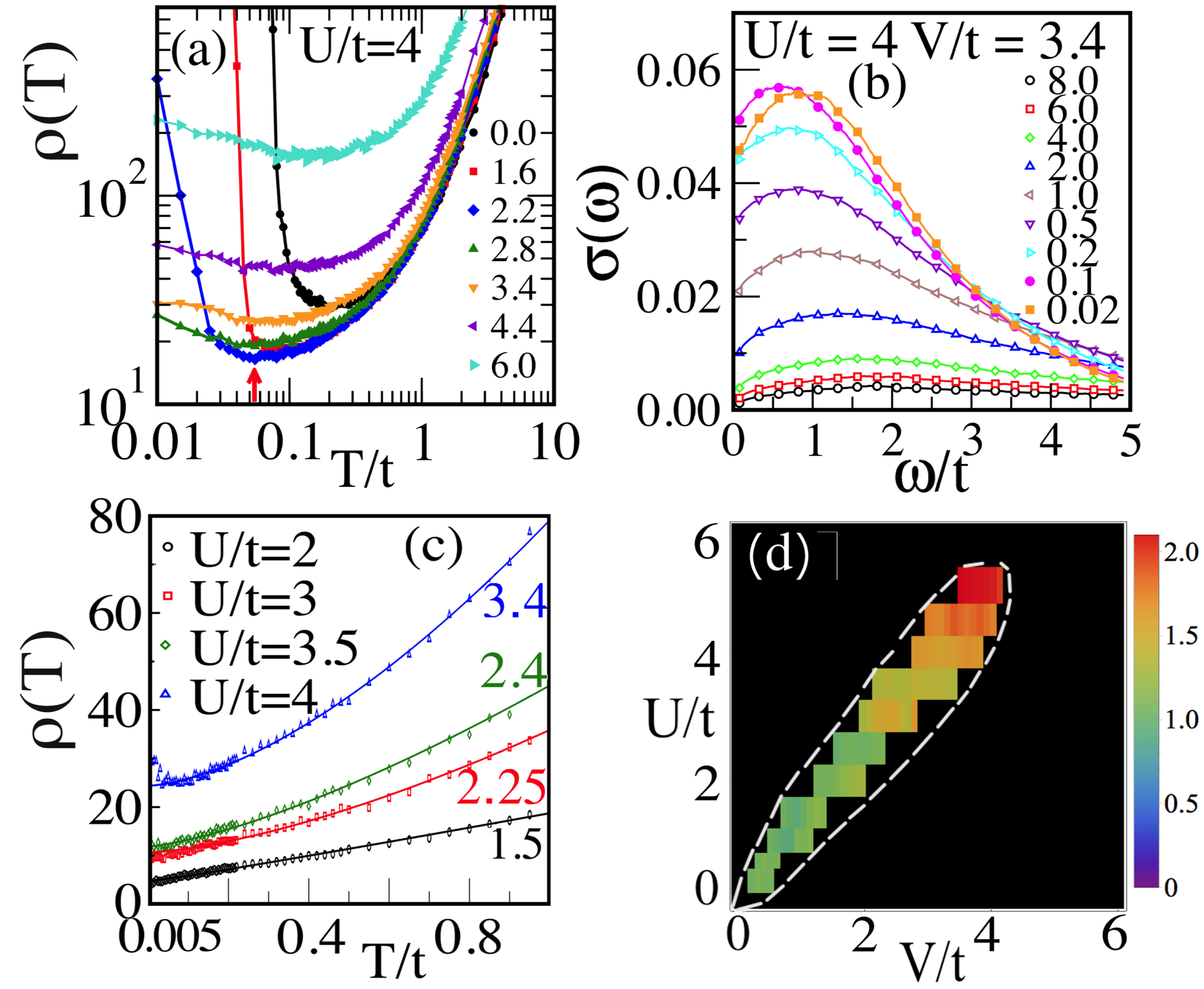
Figure 3: (color online) (a) $\rho$ ($\pi e^{2}/\hbar a_{0}$ units) vs. $T/t$ at $U/t=4$ and the various $V/t$’s in the column ($a_{0}$ is the lattice spacing, set to 1). The red arrow at the bottom shows $\rho_{min}$ for $V/t=3.4$. (b) Optical conductivity at $U/t=4$ and $V/t=3.4$ displaying non-Drude behavior, at the $T/t$’s in the column. (c) $\rho(T)$ at special values of $U/t$ and $V/t$ such that the state is metallic almost in all the $T/t$ range shown. Solid lines are fits to $\rho(0)+AT^{\alpha}$. For $U/t=2,~{}3,~{}3.5$, and $4.0$, and the $V/t$ values indicated (color, right), $\alpha$ is 1.02, 1.35, 1.39, and 1.68, respectively. (d) The metallic window in the $U-V$ plane at low temperature $T/t=0.005$ is shown by the colored region (the dashed line just guides the eye). The black region denotes insulator. The color of the metallic region depicts the value of $\alpha$ arising from the $T^{\alpha}$ scaling of $\rho(T)$.

Figure 2 (d) shows $\omega\sigma(\omega)$ at $T=0$ for different disorder values covering the Mott-Insulator, the strange metal, and the large disorder (CA-I) phases. For $V/t\leq 2.0$, $\sigma(\omega)$ is clearly gapped. In the narrow range $2.0<V/t<2.6$, $\omega\sigma(\omega)$ tends to zero as $\omega\rightarrow 0$ in a nonlinear manner. For $2.6\leq V/t\leq 3.8$, $\omega\sigma(\omega)\rightarrow 0$ linearly i.e. $\sigma(\omega)$ is constant at small $\omega$ indicating a metal. For the CA-I, variable range hopping is expected to provide a $\omega^{3}ln^{3}(I/\omega)$ behavior Imry (2002), where $I$ is a typical energy scale depending on the localization length. Supplementary Material Sec II Fig. 2 shows that the same behavior holds across the finite $T$ insulator to metal transitions as well. Our $T=0$ phase boundaries in Fig. 1 are in excellent agreement with earlier literature Heidarian and Trivedi (2004); Heidarian (2006) and the T = 0 metal is robust against finite size scaling (Supplementary Material, Fig. 3). We now shift the focus to our main contributions at finite $T$.

2. Non Fermi liquid metal. The resistivity extracted from $1/\sigma(\omega)$ at small $\omega$ (see supplementary) is in Fig. 3 (a) for $U/t=4$. There are several important features: (i) $d\rho/dT$ becomes positive at large $T$ for all values of $V/t$; (ii) For the PM-I regime at $V/t=0$ and 1.6, $d\rho/dT$ becomes negative with eventual divergence at the critical AFM temperature. For the metallic ($V/t=2.8$ and $3.4$) and the CA-I ($V/t=4.4$ and $6.6$) phases, $\rho(T)$ saturates at the lowest $T$’s investigated fin . (iii) There are resistivity minima at finite $T$ which coincide with the corresponding location of the peaks in $N(0)$ in Fig. 2 (c) at, e.g., $V/t=3.4$. The NFL nature of the disorder-induced metallic state can be inferred from panel (b) which shows that $\sigma(\omega)$ has a non-Drude form with a peak at finite frequency. This peak is further pushed to higher frequency with increasing $T$, except at very low $T$ when the peak converges to $\omega/t\sim 1$.

Both $\rho(T)$ here, and specific heat ($C_{v}$) in Supplementary Material Fig. 4, show low $T$ deviations from FL behavior consistent with literature on disorder induced NFL’s Miranda and Dobrosavljević (2005), justifying our ^′NFL metal^′ nomenclature.

Consider now the $\rho$ vs. $T$ behavior for the NFL state. In the metallic regime ($V/t=3.4$), the resistivity minimum occurs at $T/t\sim 0.1$. From Fig. 2 (c) at $V/t=3.4$, the location of $\rho_{min}$ coincides with the peak in $N(0)$ at $T/t\sim 0.055$. This non-monotonic dependence of $N(0)$ on $T$ agrees with DQMC studies of the Hubbard model Paiva et al. (2011) for $V=0$. The initial increase of $N(0)$ is due to thermally induced fluctuations that enhance the DOS weight at $\omega=0$. At high $T$, the scattering of fermions from the Aux. F.’s suppress $N(0)$, and this non-monotonicity is reflected in the metallic-like thermal behavior of $\rho(T)$. In summary, at low $T$ the initial increase of the DOS at the Fermi level forces $d\rho/dT$ to be negative, while at high $T$ this DOS is suppressed again because of the localized spins and $d\rho/dT$ changes sign.

3. Scaling of resistivity. In Fig. 3 (c) we show $\rho(T)$ for combinations of $U/t$ and $V/t$ where the system is a metal over a wide temperature range. The full map of the low temperature metallic region in the $U/t-V/t$ plane is in Fig. 3 (d). The resistivity data is fitted to $\rho(0)+AT^{\alpha}$ for each case to extract $\alpha$ fit (a). For small/intermediate values of $(U/t,~{}V/t)$ (open circles), $\rho(T)$ grows linearly with $T$ in the range analyzed. For larger $U/t$ (and corresponding $V/t$) $\alpha$ increases from $\sim$1.0 to $1.7$ for $U/t=2,~{}V/t=3.4$. As shown in Fig. 3 (d), the metallic window at $T/t=0.005$ occurs roughly around the line $U\sim 1.25V$ RS- (a). The dashed line guides the eye and it envelops the metallic region. The metallic-regime color scale indicates the value of $\alpha$ in the temperature fit of $\rho(T)$. For up to $U/t=2.5$, $\alpha\sim 1$ growing slowly with $U/t$ (the smallest values checked are $U/t=0.5,~{}V/t=0.5$). For larger $U/t,V/t>2.5$, $\alpha$ grows reaching a maximum value close to 2 for $U/t=5$ fit (b). This $\alpha\sim 2$ does not imply a FL but we believe it is just one of the possible transport exponents that occurs in our system in its slow evolution. For even larger $U/t$, within our precision the metallic region closes.

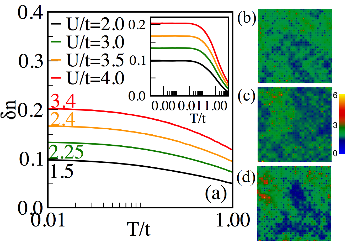
Figure 4: (color online) Fluctuations in the charge density vs. $T$ at various $U/t$’s and $V/t$’s (color), in the metallic regime. Inset contains the same data up to $T/t=10$. (b,c,d) show real-space maps of $|\psi(\boldmath{r})|^{2}$ at the Fermi energy using $32^{2}$ systems at $T/t=0.2$ and coupling strengths ($U,~{}V$) = ($2.0t$, $1.5t$), ($3.0t$, $2.25t$) and ($4.0t$, $3.4t$), respectively. Color scale indicates the range of values for $|\psi(\boldmath{r})|^{2}$ in $10^{-3}$ units. Data in (a) to (d) are averaged over 10 MC samples for a fixed disorder realization.

4. Discussion. To better understand the combined effect of disorder and interaction in the metallic phase, in Fig. 4 (a) we show the variance of the local density $\{n_{i}\}$, defined as $\delta n(U,~{}V,~{}T)=\langle\sqrt{\langle n\rangle^{2}-\langle n^{2}\rangle}\rangle$. The outer angular brackets imply averaging over MC samples at fixed $T$, while the inner ones are the quantum average within a single MC sample. There are two sources of disorder that control the variance of $\delta n(U,~{}V,~{}T)$. First is the static disorder ($V$) with variance $\delta V$ and the second are the Aux. F.’s. These Aux. F.’s directly couple to the fermions and indirectly to the disorder through the local fermion occupations (Sec. I of the Supplementary Material). Then, the Aux. F. also provide an inhomogeneous background that at low temperatures follows the presence of intrinsic static disorder. But at temperatures where $k_{B}T\geq\delta V$, the intrinsic disorder ($V$) is unimportant and the Aux. F. configurations become homogeneous in average. Thus, $\delta n(U,~{}V,~{}T)$ remains non zero at low $T$ while it tends to zero at large $T$, on MC sample averaging. This behavior is observed in the inset of Fig. 4 (a). In the main panel we show the same data between $T/t=0.01$ and $1$. We find a systematic increase in $\delta n(U,~{}V,~{}T)$ with increasing $U/t$ and $V/t$. This variance manifests as real-space charge clusters as shown in Fig. 4 (b) to (d) that contains maps of $|\psi(\boldmath{r})|^{2}$ at fixed $T$, MC sample averaged, for states at the Fermi energy. With increasing $U/t$ and $V/t$, the charge clustering and the charge fluctuations magnitude increase systematically following the increase in $\delta n(U,~{}V,~{}T)$. This provides a controlled enhancement in spatially inhomogeneous background from which the fermions scatter RS- (b).

It is known that fermions coupled to classical variables such as disorder Kumar and Majumdar (2005a), adiabatic phonons Blawid et al. (2003) etc. can exhibit charge clustering, metallic glasses, and NFL behavior. In our case, not only the quenched disorder but also the Aux. F. fluctuations play the role of the classical scatterer that give rise to NFL scaling. Such charge clusters and NFL behavior has been experimentally observed in the 2DEG near a $T=0$ quantum critical point Bogdanovich and Popović (2002); Jaroszyński et al. (2002); Kravchenko and Sarachik (2004). Here, within MF-MC, we have found such a “charge cluster metal” in the half-filled Anderson Hubbard model and also observed that their deviation from FL theory can be tuned. This tunability allows us to show that, in a single model Hamiltonian, the resistivity scaling with $T$ can vary between linear to near quadratic, features observed in real NFLs like cuprates and heavy fermions. Our results thus represent progress towards identifying a single model system with NFL behavior transcending many material families.

Acknowledgments. A. Mukherjee acknowledges useful discussions with P. Majumdar, P. Chakraborty, and H. R. Krishnamurthy. N.P. and N.K. were supported by the National Science Foundation, under Grant No. DMR-1404375. E.D. and A. Moreo were supported by the U.S. Department of Energy, Office of Basic Energy Sciences, Materials Sciences and Engineering Division.

Supplementary material

I I.   Model and Method

In this section we discuss the Mean field-Monte Carlo (MF-MC) method. The approach properly incorporates thermal fluctuations in a mean field theory and has been shown to reproduce accurately the properties of the clean-limit Hubbard model when compared with Determinantal Quantum Monte Carlo (DQMC) results Mukherjee et al. (2014). MF-MC allows for efficient simulations on large lattices Mukherjee et al. (2015) and has also been used to study frustrated systems Tiwari and Majumdar (2014); Swain et al. (2016), the BCS-BEC crossover Karmakar and Majumdar (2016a); Tarat and Majumdar (2015), imbalanced Fermi gases Karmakar and Majumdar (2016b), and the multiorbital Hubbard model Mukherjee et al. (2016); Swain and Majumdar (2016). Below we present detailed account of the formalism, its numerical implementation, benchmarks against clean system DQMC results, observables calculated and typical parameters (system size, broadening etc.) used in the present calculation.

1. Effective spin-fermion from the Hubbard model: As mentioned in the main paper, for our study we use the Anderson-Hubbard model on a square lattice at half filling ($n=1$). The Hamiltonian is:

$$\begin{split}H&=-t\sum_{\langle i,j\rangle\ \sigma}c^{\dagger}_{i,\sigma}c^{\phantom{\dagger}}_{i,\sigma}+\sum_{i}Un_{i\uparrow}n_{i\downarrow}\\ &+\sum_{i}(V_{i}-\mu)(n_{i\uparrow}+n_{i\downarrow}),\end{split}$$ (1)

where the first term is the kinetic energy and the second term is the standard Hubbard repulsion. $c^{\phantom{\dagger}}_{i\sigma}$ ( $c^{\dagger}_{i\sigma}$) annihilates (creates) an electron at site $i$ with spin $\sigma$. The number operator is $n_{i\sigma}=c^{\dagger}_{i\sigma}c^{\phantom{\dagger}}_{i\sigma}$. The disorder $V_{i}$ at each site is chosen randomly in the interval $[-V,V]$ with a uniform probability. We perform a rotationally invariant decoupling of the interaction term and use the Hubbard-Stratonovich (HS) decomposition to obtain an effective Hamiltonian under the approximations described below. Briefly, the rotational invariant form for the interaction term gives

$$n_{i,\uparrow}n_{i,\downarrow} = \frac{1}{4}(n_{i}^{2})-S_{iz}^{2}$$ (2)

$$= \frac{1}{4}(n_{i}^{2})-({\mathbb{S}}_{i}\cdot\hat{\Omega}_{i})^{2}.$$

Here, the spin operator is ${\mathbb{S}_{i}}=\frac{\hbar}{2}\sum_{\alpha,\beta}c^{\dagger}_{i,\alpha}{\mathbb{\sigma}}^{\phantom{\dagger}}_{\alpha,\beta}c^{\phantom{\dagger}}_{i,\beta}$, $\hbar=1$, $\{\sigma^{x},\sigma^{y},\sigma^{z}\}$ are the Pauli matrices, and $\hat{\Omega}$ is an arbitrary unit vector. To decouple this term we introduce two auxiliary fields $\bm{m}_{i}(\tau)$ and $\phi_{i}(\tau)$ at every site $i$ and every imaginary time $\tau$, with each auxiliary field coupled to the spin and the charge degrees of freedom, respectively. In our recent work Mukherjee et al. (2014) we showed that for $V_{i}=0$, if we consider time independent auxiliary fields and replace the $\phi_{i}$ auxiliary field by its saddle point value, $\phi_{i}=-i\frac{U}{2}\langle n_{i}\rangle$, we obtain the first three terms of the effective Hamiltonian in Eq. 3. Since the disorder term is a one-body interaction it remains unchanged from Eq. 1 to Eq. 3:

$$\begin{split}H_{eff}&=-t\sum_{\langle i,j\rangle\ \sigma}c^{\dagger}_{i,\sigma}c^{\phantom{\dagger}}_{i,\sigma}+\frac{U}{2}\sum_{i}(\langle n_{i}\rangle n_{i}-\textbf{m}_{i}.\sigma_{i})\\ &+\frac{U}{4}\sum_{i}(\textbf{m}_{i}^{2}-\langle n_{i}\rangle^{2})+\sum_{i}(V_{i}-\mu)(n_{i\uparrow}+n_{i\downarrow}).\end{split}$$ (3)

Equation 3 is, thus, a one-body Hamiltonian that belongs to the spin fermion class as it is a functional of the classical auxiliary fields $\{\bm{m}_{i}\}$. We note that although there is no direct coupling between the auxiliary fields $\{\bm{m}_{i}\}$ and the disorder, there is an indirect coupling through the fermion density which is sensitive to the disorder profile and are in turn coupled to the auxiliary fields $\{\bm{m}_{i}\}$.

At $T=0$, $H_{eff}$ reduces to a mean field Hamiltonian while at finite $T$, admitting thermal fluctuations (via employing a Monte Carlo scheme as discussed below) renders the calculation much better than a simple finite $T$ mean-field theory. These conclusions are based on results shown below and in previous literature. Because of the mixing of mean field theory and Monte Carlo, we call the method the “Mean Field-Monte Carlo” (MF-MC) approach.

2. Treatment of the spin-fermion model:

Our strategy for solving the resulting spin-fermion model is as follows. We aim to generate equilibrium configurations of $\{\bm{m}_{i}\}$ at a given temperature that minimizes the free energy of the system. The free energy of course contains a quantum component for which we diagonalize $H_{eff}$ for a given configuration $\{\bm{m}_{i}\}$. Since we have broken translation invariance by the quenched disorder, we cannot set $\langle n_{i}\rangle=1$ as could be done in the half filling clean problem. Thus, the values of $\langle n_{i}\rangle$ need to be determined at each iteration. Only then we can diagonalize $H_{eff}$. For this task, we start with an average value of $\langle n_{i}\rangle=1$ at the beginning of our calculation at high $T$. We then choose a random value set of the Aux.F. and diagonalize $H_{eff}$ and extract the associated eigenvalues. We then add the purely classical term $\frac{U}{4}\sum_{i}\textbf{m}_{i}^{2}$ to the fermionic energy. The final free energy is then used within a Metropolis algorithm to update the $\{\bm{m}_{i}\}$ variables. By this repeated process the static auxiliary fields $\{\bm{m}_{i}\}$ are annealed with a classical Monte-Carlo (MC). We repeat the classical MC system sweep 50 times. We then stop updating the Aux.F. and run a self consistency loop for the $\langle n_{i}\rangle$ in the fixed Aux. F. background. Once the $\langle n_{i}\rangle$ have converged for all the sites we stop the self consistency and again run the classical MC for the Aux. F. now for the fixed $\langle n_{i}\rangle$ configuration. The $\langle n_{i}\rangle$ self consistency is repeated after every 50 steps of the classical MC system sweeps during the thermalization portion of the classical MC. This usually consists of 2000 MC system sweeps. During the measurement steps, namely another 2000 MC system sweeps at the same temperature, the density is no longer adjusted, as we found that observables are not sensitive to the self consistency after the first 2000 MC system sweeps. The process then is repeated at successive lower $T$, where we use the $\langle n_{i}\rangle$ and Aux. F. configurations of the last system sweep of the higher $T$ as the initial condition for the lower temperature. This is a computational demanding procedure that requires hundreds of nodes because of the fine grid in $U$, $V$, and $T$ required plus the average over quenched disorder configurations.

To summarize, the static auxiliary fields $\{\bm{m}_{i}\}$ are annealed with a classical Monte-Carlo (MC) while the fermion problem is solved by ED, with some self consistency steps to obtain $\langle n_{i}\rangle$. The chemical potential $\mu$ is freely adjusted to fix the global density to half filling. We performed a total of 4000 MC system sweeps at every temperature from which 200 of the last 2000 were used to calculate the observables discussed below and in the main paper. We begin MC simulation at high temperature, usually ($T/t=1.0$) with a random configuration of auxiliary variables $\{\bm{m}_{i}\}$ and then cool down to a lowest temperature of ($T/t\sim 5\times 10^{-3}$), where up to $100$ intermediate temperatures are used to allow for a gradual evolution in the configurations allowing us to avoid potential metastable states. The observables are averaged over 10 to 20 quenched disorder realizations.

To study the effects of random disorder on a strongly interacting system, it is important to consider large lattices. We use a variant of the above mentioned ED+MC technique known as the traveling cluster approximation (TCA) Kumar and Majumdar (2006) that can be easily parallelized to access large system sizes Mukherjee et al. (2015). We mainly present results for $32^{2}$ systems although some of our results were cross checked on lattices up to $56^{2}$. We used the thermalized configurations of the auxiliary fields and the corresponding eigenvalues and eigenvectors to calculate various observables: density of states $N(\omega$), magnetic structure factor in real and momentum space $S(\textbf{q})$ and $C(|{\mathbb{r}}|)$, respectively, real-space maps of charge densities ($|\psi(\bm{r_{i}},E_{F})|^{2}$)) for states at the Fermi energy, inverse participation ratio ($|\psi(E_{F})|^{4}$) at Fermi energy and optical conductivity ($\sigma(\omega)$) using the Kubo-Greenwood formula. We also extract the resistivity ($\rho$) vs. temperature. We discuss these observables in detail in the next section.

List of suppfigures 1 (color online) (a) The $T/t-U/t$ phase diagram for the one-band Hubbard model. The solid red squares show the dependence of $T_{N}$ on $U/t$ obtained using the MF-MC technique on $4^{3}$ clusters. The crosses are estimations of $T_{N}$ obtained from finite-size scaling. The AF-I region denotes the Néel type AFM phase with long-range order and insulating characteristics. The open squares are the $T_{N}$ obtained from the DQMC method, from Ref. Staudt et al., 2000. The light blue region depicts the regime of preformed local moments above the AF-I phase. The dashed line shows the $T_{N}$ obtained from the simplistic Hartree-Fock calculation at finite temperature where the critical temperature incorrectly grows linearly with $U/t$ at large $U/t$. (b) Magnitude of the auxiliary classical fields averaged over the lattice ($\langle|\textbf{m}|\rangle$) vs. temperature for the $U/t$ values shown in (c). At large temperature the thermal fluctuations cause ($\langle|\textbf{m}|\rangle$) to grow linearly with temperature for all the $U$’s shown (inset). The reason for this temperature dependence of $\langle|\textbf{m}|\rangle$ and its correlation with $N(\omega=0)$ is discussed in the text. (c) Shows $N(\omega=0)$ for different $U/t$ values. This non monotonicity was reported before in a DQMC study, see Ref. Paiva et al., 2001.

The MF-MC method can be used to study the Hubbard model at arbitrary coupling and temperature and is free of the sign problem. The MF-MC approach has been extensively benchmarked against Determinantal Quantum Monte-Carlo for the Hubbard model Mukherjee et al. (2014) and its $t-t^{\prime}$ variant. Also the method can be parallelized to allow access to very large lattices Mukherjee et al. (2015) up to $250^{2}$ in two dimensions for the one-band Hubbard model.

Finally, establishing the phase diagram on a fine $V$, $U$ and $T$ grid, involving also the averaging of the data over many disorder realizations, demanded a substantial computational effort. Each disorder configuration, for a single set of $U$ and $V$ on a 32² system, requires $\sim 1500$ cpu hours for running the simulation with 100 temperature points. This is multiplied by a factor of 20 for averaging over disorder realizations. Finally, for the full $U$-$V$ phase diagram 400 ($U$, $V$) combinations were used. In addition, calculation of disorder averaged optical conductivity, that scales as $L^{3}$, $L=32^{2}$, for every $(U,V)$ set, also added substantial numerical cost. This was possible due to access to the large cluster computing facility (Newton) at the University of Tennessee, Knoxville.

I.1 Observables

(i) Static magnetic structure factor: Information regarding the Néel antiferromagnet order is found by computing the static magnetic structure factor. Here we focus on the wavevector $\bm{q}=(\pi,\pi)$ as that is the expected order at half-filling for any finite value of $U$. The spins ${\mathbb{S}_{i}}$ are constructed from the eigenvectors of the equilibrated configurations. Below the magnetic ordering temperature, the electronic spin degree of freedom are enslaved to magnetic auxiliary variables $\bm{m}_{i}$. Thus, it is interesting to note that even a magnetic structure factor constructed only out of the magnetic auxiliary fields closely resembles the full spin structure factor. The static magnetic structure factor is defined as:

$$S({\mathbb{q}})=\frac{1}{N^{2}}\displaystyle\sum\limits_{i,j}e^{i{\mathbb{q}}\cdot({\mathbb{r}}_{i}-{\mathbb{r}}_{j})}\langle{{\mathbb{S}_{i}}\cdot{\mathbb{S}_{j}}}\rangle,$$ (4)

where ${\mathbb{q}}=\{\pi,\pi\}$ is the wavevector of interest. The normalization $N^{2}$ is equal to $L^{4}$, where $L$ is the linear dimension of a $L^{2}$ system.

(ii) Density of states: We calculate the density of states (DOS), $N(\omega)=\sum_{m}\delta(\omega-\omega_{m})$, where $\omega_{m}$ are the eigenvalues of the fermionic sector and the summation runs up to $2L^{2}$, i.e. the total number of eigenvalues of a $L^{2}$ system with spin. $N(\omega)$ is calculated by implementing the usual Lorentzian representation of the $\delta$ function. The broadening needed to obtain $N(\omega)$ from the Lorentzians is $\sim BW/2L^{2}$, where $BW$ is the fermionic bandwidth at $U=0$. Numerically for the 32² system, the broadening is about $0.004t$. Hundred $N(\omega)$ samples are obtained from the 4000 measurement system sweeps at every temperature. The 200 $N(\omega)$ samples are used to obtain the thermally averaged $\langle N(\omega)\rangle_{T}$ at a fixed temperature. These are further averaged over data obtained from 10-20 independent runs with different random number seeds. We also plot $N(\omega-\mu=0)$ vs temperature and disorder.

(iii) Real space $q=(\pi,\pi)$ magnetic correlations: We also calculate the real space correlation function between the ${\mathbb{S}_{i}}$ vectors. This correlation function is defined as,

$$C(|{\mathbb{r}}|)=\frac{1}{P}\sum\limits_{|{\mathbb{r}}|=|{\mathbb{i}}-{\mathbb{j}}|,a}(-1)^{|{\mathbb{i}}-{\mathbb{j}}|}\langle S^{a}_{i}S^{a}_{j}\rangle.$$ (5)

In $C(|{\mathbb{r}}|)$ the summation runs over all P pairs of sites at a distance $|{\mathbb{r}}|$ and is normalized accordingly. The sum over $a$ runs over the three directions $x$, $y$, and $z$. This indicator is used to investigate short range magnetic order in the system in real space.

(iv)Transport calculations: The d.c conductivity $\sigma_{dc}$ is estimated by the Kubo-Greenwood expression Mahan (1990) for the optical conductivity. In a one-electron model system:

$$\sigma(\omega)=\frac{\pi e^{2}}{N\hbar a_{0}}\sum_{\alpha,\beta}(n_{\alpha}-n_{\beta})\frac{|f_{\alpha\beta}|^{2}}{\epsilon_{\beta}-\epsilon_{\alpha}}\delta(\omega-(\epsilon_{\beta}-\epsilon_{\alpha})).$$ (6)

The $f_{\alpha\beta}$ are the matrix elements of the current operator, e.g., $\langle\psi_{\alpha}|j_{x}|\psi_{\beta}\rangle$, and the current operator itself (in the tight-binding model) is given by $j_{x}=ita_{0}e\sum_{i,\sigma}(c^{\dagger}_{{i+a_{0}\hat{x}},\sigma}c^{\phantom{\dagger}}_{i,\sigma}-h.c)$. The $\psi_{\alpha}$ are single-particle eigenstates, and $\epsilon_{\alpha}$ are the corresponding eigenvalues. The $n_{\alpha}=f(\mu-\epsilon_{\alpha})$ are Fermi factors.

We can compute the low-frequency average, $\sigma_{av}(\mu,\Delta\omega,N)=(\Delta\omega)^{-1}\int_{0}^{\Delta\omega}\sigma(\mu,\omega,N)d\omega$, using periodic boundary conditions in all directions. The averaging interval is reduced with increasing $N$, with $\Delta\omega\sim B/N$. Here the constant $B$ is fixed by setting $\Delta\omega=0.008t$ at $N=32^{2}$. Ideally, the d.c. conductivity is finally obtained as $\sigma_{dc}(\mu)={\lim}_{L\rightarrow\infty}{\sigma}_{av}(\mu,B/L,L)$. However, given the extensive numerical cost of our calculation, we simply use the result of $32^{2}$ system as our $\sigma_{dc}(\mu)$. The chemical potential is set to target the required electron density $n$. This approach to d.c. transport calculations has been benchmarked in a previous work Kumar and Majumdar (2005b).

List of suppfigures 2 (color online) Optical conductivity data at finite (high) temperatures. Plots show $\omega\sigma(\omega)$ vs $\omega$ for $U=4t$, different disorder strengths, and the temperature values indicated for each $V/t$. In the left panel (a) the orange curve displays nonlinear behavior at low $T$ (Mott phase). At higher $T$ we observe a linear behavior, thus a metal. In the middle panel (b), we find linear behavior at all $T$ (i.e. the system is metallic all through). At larger $V$, the high $T$ data shows linearity, indicating a metal, while the low $T$ data show clear deviations from linear behavior. All panels are for $U/t=4$ and using a $32^{2}$ system. Solid black lines are guides to the eye in all panels.

I.2 Half-filled Hubbard model: Results $\&$ benchmarking against DQMC

In this section, we briefly reproduce some pertinent results from earlier publications on the finite temperature properties of the half-filled Hubbard model at zero disorder Mukherjee et al. (2014). We wish to establish a comparison with DQMC for the finite $T$ properties and to discuss the nature of auxiliary field fluctuations with $T$.

1. Zero disorder phase diagram: Figure 1 (a) shows the $U-T$ phase diagram at half filling on a three-dimensional $4^{3}$ lattice from our earlier work Mukherjee et al. (2014). The shaded region (below) solid square symbols is a $(\pi,\pi,\pi)$ antiferromagnetic Mott insulator. The solid squares are obtained using our approach and the open square symbols are DQMC results Staudt et al. (2000). The dashed line with triangles are the $T_{N}$ obtained within finite temperature Hartree-Fock formalism. Clearly, our approach captures the correct non monotonic behavior of $T_{N}$ with $U$ and has semiquantitative agreement with DQMC. This is much better than simple finite temperature Hartree-Fock that gives qualitatively incorrect results. In addition the blue shaded region corresponds to preformed local moments, another feature that a simplistic finite $T$ mean-field theory cannot capture. The gray region to the left of the preformed local moments area is a PM-M. Also as shown in our previous work Mukherjee et al. (2014), the MF-MC approach can capture the two peak specific heat related to moment formation and moment ordering.

2. Auxiliary field fluctuations at zero disorder: As discussed above, the auxiliary fields $\{\bm{m}_{i}\}$ couple linearly to the fermions and they have a quadratic classical cost as well (See Eq. 3). In Fig. 1 (b) we show the system averaged (auxiliary fields) $\{\bm{m}_{i}\}$ as a function of temperature up to $T=100t$ (in the inset) and up to $T=5t$ in the main panel. The data is shown for different $U$’s as indicated in panel (b). For $U=4t$ at low $T$, the $\{\bm{m}_{i}\}$ fields are enslaved to the magnetic moment and thus have a fixed value. With increasing $T$, the magnetic moments weakened and so does $\{\bm{m}_{i}\}$. At $T_{N}=0.12t$, the system is in a paramagnetic metallic state (the gray region in Fig. 1). At higher temperatures with negligible local moments, the value of $\langle|\textbf{m}|\rangle$ is governed by thermal fluctuations. At these temperatures the auxiliary fields behave as harmonic oscillators with a mean amplitude proportional to $\sqrt{T/U}$. Thus, $\langle|\textbf{m}|\rangle$ grows with increasing temperature. With increasing $U$, the dominance of thermal fluctuations in governing $\langle|\textbf{m}|\rangle$ is pushed to progressively higher temperatures that increase with $U$.

This unrestricted growth of the Aux. F. at very high $T$ is unavoidable in the continuous Hubbard-Stratonovich based MF-MC. However, to compare with DQMC, where the magnitude of the Aux. F are fixed to 1, we restrict the comparison to a temperature range for which $\langle|\textbf{m}|\rangle\leq 1$. For all data of focus in our publication, particularly with regards to the temperature scaling of $\rho(T)$, we are in a regime where $\langle|\textbf{m}|\rangle\leq 1$.

In panel (c) we show the clean limit $N(0)$ vs $T$. We find that the temperature where $N(0)$ has a peak coincides with both the $T_{MIT}$ in Fig.1 (a) and the temperature where $\langle|\textbf{m}|\rangle$ start growing as $\sqrt{(T/U)}$. This suggests that auxiliary field amplitude fluctuations are the main scattering effect in the zero disorder problem at high temperature. This non monotonic dependence of $N(0)$ has been found in DQMC calculations as well. In the main text, we show that the same qualitative behavior holds even in the presence of disorder.

List of suppfigures 3 (color online) Finite size scaling plots for inverse participation ratio for three disorder values $V/t$, at $U/t=4$. $V=2.5$ and 4.8 correspond to insulating phases while 3.6 corresponds to the metallic phase. The IPR vanishes for the metal and converges to a finite value for the insulator phases as $L\rightarrow\infty$. Dashed lines are a guide to the eye.

II II.  Anderson Hubbard model: determining metal insulator boundary

As mentioned in the main paper, the slope of the resistivity vs temperature is not a good criterion to decide between metals and insulators in strongly correlated systems with disorder. Thus, we have used the behavior of the optical conductivity vs frequency ($\omega/t$) at small frequency as an indicator of metal insulator transitions. As discussed in the main paper, we look for linear behavior of $\omega\sigma(\omega)$ with $\omega$. This ensures a constant conductivity close to $\omega/t=0$. Previously at $T=0$ this criterion has been often employed to decide between metal and insulator Heidarian and Trivedi (2004). In Fig. 2 (d) of the main paper we have shown the corresponding data from our calculations to determine the low temperature (in our case $T/t=0.005$) metal insulator boundary. In this Supplementary Material Fig. 2 (a) to (c), we show typical supporting data that we have used to determine the finite-temperature metal insulator boundary for $U/t=4$. In (a), the $V=0$ case is shown. The straight (black) line is a guide to the eye. We see a clear departure from linear dependence for $T/t=0.08$, while for $T/t=0.2$ the linear behavior is recovered. In (b) we show the data for $V/t=3.4$ which is in the metallic regime. Here we see that, as in the main text Fig 2 (d), for $V/t=3.4$ at $T/t=0.005$ the linear behavior continues at all explored temperatures (we have checked this up to $T/t=2$). The highest $T$ data shown here is $T/t=0.5$. In (c) we show that the deviation from linearity reduces with increasing $T$ for the CA-I phase as well. In the data shown, $T/t=1.2$ is a metal while the lower $T$ system is insulating.

List of suppfigures 4 (color online) $C_{v}/T$ vs temperature for the disorder induced metal. The main panel shows data from $T/t=0.3$ to $T/t=0.9$ for three disorder values $V/t$ (indicated) and for $U/t=4$. The solid lines are fits to $\gamma_{0}Log(T/T_{0})$. The inset shows the same data from $T/t=0.1$ to $1.0$. The data for $V/t=2.6$ and $V/t=3.4$ are respectively shifted down and up by 15, in both the main panel and the inset for clarity.

At $T/t=0.005$, we also calculated the inverse participation ratio (IPR) for states at the Fermi energy ($E_{F}$). In practice we averaged over a few states in a small window around the $E_{F}$. This is done for two reasons. Firstly, it allows an alternative independent way to cross check the metal insulator boundaries at low $T$. Secondly, numerically this calculation is much less expensive than calculating $\sigma(\omega)$. Thus, at least at low $T$ we could perform standard finite size scaling to show that IPR extrapolates to zero for the metallic phase and converges to a finite value for both the M-I and the CA-I phases. The data is shown in Fig. 3.

III III.  Specific heat vs temperature

Figure 4 shows the evolution of the specific heat ($C_{v}$) with temperature for the disorder-induced metallic phase. As seen in the main panel, $C_{v}/T$ has a $Log(T/T_{0})$ dependence on temperature over a wide temperature range. This behavior holds true for all the three cases of disorder-induced metal shown in the figure. The specific heat at $T/t<0.3$ diverges at a faster rate. Thus, our calculation also captures another hallmark of a non Fermi liquid, e.g. the divergence of the specific heat with decreasing temperature, in contrast to FL behavior.

Details of the variations in $\gamma_{0}$ and $T_{0}$, in the range of logarithmic scaling of $C_{v}/T$, will be reported elsewhere.

References

- Gegenwart et al. (1998) P. Gegenwart et al., Phys. Rev. Lett. 81, 1501 (1998).
- Trovarelli et al. (2000) O. Trovarelli et al., Phys. Rev. Lett. 85, 626 (2000).
- Julian et al. (1996) S. R. Julian et al., J. Phys.: Condens. Matter 8, 9675 (1996).
- Coleman et al. (2001) P. Coleman, C. Pepin, Q. Si, and R. Ramazashvili, J. Phys.: Condens. Matter 13, R723 (2001).
- Jaramillo et al. (2014) R. Jaramillo, S. D. Ha, D. M. Silevitch, and S. Ramanathan, Nature Physics 10, 304 (2014).
- Lahoud et al. (2014) E. Lahoud, O. N. Meetei, K. B. Chaska, A. Kanigel, and N. Trivedi, Phys. Rev. Lett. 112, 206402 (2014).
- Damascelli et al. (2003) A. Damascelli, Z. Hussain, and Z.-X. Shen, Rev. Mod. Phys. 75, 473 (2003).
- Hussey et al. (2003) N. E. Hussey, M. Abdel-Jawad, A. Carrington, A. P. Mackenzie, and L. Balicas, Nature 425, 814 (2003).
- Keimer et al. (2015) B. Keimer, S. A. Kivelson, M. R. Norman, S. Uchida, and J. Zaanen, Nature 518, 179 (2015).
- Anderson (2006) P. Anderson, Nature Physics 2, 626 (2006).
- Casey and Anderson (2011) P. A. Casey and P. W. Anderson, Phys. Rev. Lett. 106, 097002 (2011).
- Bogdanovich and Popović (2002) S. c. v. Bogdanovich and D. Popović, Phys. Rev. Lett. 88, 236401 (2002).
- Jaroszyński et al. (2002) J. Jaroszyński, D. Popović, and T. M. Klapwijk, Phys. Rev. Lett. 89, 276401 (2002).
- Kravchenko and Sarachik (2004) S. V. Kravchenko and M. P. Sarachik, Reports on Progress in Physics 67, 1 (2004).
- Arrachea et al. (2004) L. Arrachea, D. Dalidovich, V. Dobrosavljević, and M. J. Rozenberg, Phys. Rev. B 69, 064419 (2004).
- Dalidovich and Dobrosavljević (2002) D. Dalidovich and V. Dobrosavljević, Phys. Rev. B 66, 081107 (2002).
- Sachdev and Read (1996) S. Sachdev and N. Read, J. Phys.: Condens. Matter 8, 9723 (1996).
- Miranda and Dobrosavljević (2005) E. Miranda and V. Dobrosavljević, Reports on Progress in Physics 68, 2337 (2005).
- Deng et al. (2013) X. Deng, J. Mravlje, R. Žitko, M. Ferrero, G. Kotliar, and A. Georges, Phys. Rev. Lett. 110, 086401 (2013).
- Imry (2002) Y. Imry, Introduction to Mesoscopic Physics (Oxford University Press on Demand, 2002).
- Dobrosavljevic et al. (2012) V. Dobrosavljevic, N. Trivedi, and J. James M Valles, Conductor Insulator Quantum Phase Transitions, edited by V. Dobrosavljevic, N. Trivedi, and J. M. Valles Jr (Oxford University Press, 2012).
- Song et al. (2008) Y. Song, R. Wortis, and W. A. Atkinson, Phys. Rev. B 77, 054202 (2008).
- Semmler et al. (2010) D. Semmler, K. Byczuk, and W. Hofstetter, Phys. Rev. B 81, 115111 (2010).
- Tanasković et al. (2003) D. Tanasković, V. Dobrosavljević, E. Abrahams, and G. Kotliar, Phys. Rev. Lett. 91, 066603 (2003).
- Aguiar et al. (2008) M. C. O. Aguiar, V. Dobrosavljević, E. Abrahams, and G. Kotliar, Physica B: Condensed Matter 403, 1417 (2008).
- Otsuka and Hatsugai (2000) Y. Otsuka and Y. Hatsugai, J. Phys.: Condens. Matter 12, 9317 (2000).
- Srinivasan et al. (2003) B. Srinivasan, G. Benenti, and D. L. Shepelyansky, Phys. Rev. B 67, 205112 (2003).
- Chakraborty et al. (2007) P. B. Chakraborty, P. J. H. Denteneer, and R. T. Scalettar, Phys. Rev. B 75, 125117 (2007).
- Kotlyar and Das Sarma (2001) R. Kotlyar and S. Das Sarma, Phys. Rev. Lett. 86, 2388 (2001).
- Heidarian and Trivedi (2004) D. Heidarian and N. Trivedi, Phys. Rev. Lett. 93, 129901 (2004).
- Kravchenko et al. (1995) S. V. Kravchenko, W. E. Mason, G. E. Bowker, J. E. Furneaux, V. M. Pudalov, and M. D’Iorio, Phys. Rev. B 51, 7038 (1995).
- Sarma et al. (1998) D. D. Sarma et al., Phys. Rev. Lett. 80, 4004 (1998).
- Nakatsuji et al. (2004) S. Nakatsuji, V. Dobrosavljević, D. Tanasković, M. Minakata, H. Fukazawa, and Y. Maeno, Phys. Rev. Lett. 93, 146401 (2004).
- Sanchez-Palencia and Lewenstein (2010) L. Sanchez-Palencia and M. Lewenstein, Nature Physics 6, 87 (2010).
- (35) While our many-body techniques capture order-parameter fluctuations, they do not include spin-flip processes characteristics of Kondo screening effects of local moments, e.g. E. Miranda et al., Phys. Rev. Lett. 78, 290 (1997) and S. Sen et al., Phys. Rev. B 94, 235104 (2016). Thus our effort is complementary to other previous calculations.
- (36) The slight upturn in at small is compatible with the discussion in M. Ulmke, et. al. Phys. Rev. B 51 10411 (1995).
- Heidarian (2006) D. Heidarian, Metal-Insulator Transitions In Two Dimensions, Ph.D. thesis, School of Natural Sciences Tata Institute of Fundamental Research Mumbai (2006).
- (38) Since our calculation is on finite system and the lowest temperature accessed is , the expected divergence in as for the CA-I is not captured. Thus the optical conductivity data is the best indicator of metal vs insulator.
- Paiva et al. (2011) T. Paiva, Y. L. Loh, M. Randeria, R. T. Scalettar, and N. Trivedi, Phys. Rev. Lett. 107, 086401 (2011).
- fit (a) There is a also a variation in with for a fixed , details will be reported elsewhere as this is not the central issue being addressed here.
- RS- (a) In the absence of quantum () and thermal () fluctuations, the line is special, separating a phase with all sites singly occupied from another phase with a mixture of occupancies. This is why our metallic phase is close to .
- fit (b) Resistivity minimum occurs for all the cases but is pushed to lower temperatures for smaller , so the fitting is done in the regime where going up to .
- RS- (b) Extensions of the present work may include other forms of disorder (hoppings, etc.) as explored in literature Denteneer et al. (2001); Denteneer and Scalettar (2003).
- Kumar and Majumdar (2005a) S. Kumar and P. Majumdar, Phys. Rev. Lett. 94, 136601 (2005a).
- Blawid et al. (2003) S. Blawid, A. Deppeler, and A. J. Millis, Phys. Rev. B 67, 165105 (2003).
- Denteneer et al. (2001) P. J. H. Denteneer, R. T. Scalettar, and N. Trivedi, Phys. Rev. Lett. 87, 146401 (2001).
- Denteneer and Scalettar (2003) P. J. H. Denteneer and R. T. Scalettar, Phys. Rev. Lett. 90, 246401 (2003).
- Mukherjee et al. (2014) A. Mukherjee, N. D. Patel, S. Dong, S. Johnston, A. Moreo, and E. Dagotto, Phys. Rev. B 90, 205133 (2014).
- Mukherjee et al. (2015) A. Mukherjee, N. D. Patel, C. Bishop, and E. Dagotto, Phys. Rev. E 91, 063303 (2015).
- Tiwari and Majumdar (2014) R. Tiwari and P. Majumdar, EPL (Europhysics Letters) 108, 27007 (2014).
- Swain et al. (2016) N. Swain, R. Tiwari, and P. Majumdar, Phys. Rev. B 94, 155119 (2016).
- Karmakar and Majumdar (2016a) M. Karmakar and P. Majumdar, Phys. Rev. A 93, 053609 (2016a).
- Tarat and Majumdar (2015) S. Tarat and P. Majumdar, Eur. Phys. J. B 88, 68 (2015).
- Karmakar and Majumdar (2016b) M. Karmakar and P. Majumdar, Eur. Phys. J. D 70, 220 (2016b).
- Mukherjee et al. (2016) A. Mukherjee, N. D. Patel, A. Moreo, and E. Dagotto, Phys. Rev. B 93, 085144 (2016).
- Swain and Majumdar (2016) N. Swain and P. Majumdar, arXiv:1610.00695 (2016).
- Kumar and Majumdar (2006) S. Kumar and P. Majumdar, Eur. Phys. J. B 50, 571 (2006).
- Staudt et al. (2000) R. Staudt, M. Dzierzawa, and A. Muramatsu, Eur. Phys. J. B 17, 411 (2000).
- Paiva et al. (2001) T. Paiva, R. T. Scalettar, C. Huscroft, and A. K. McMahan, Phys. Rev. B 63, 125116 (2001).
- Mahan (1990) G. D. Mahan, Quantum Many Particle Physics (Plenum Press, New York, 1990).
- Kumar and Majumdar (2005b) S. Kumar and P. Majumdar, Eur. Phys. J. B 46, 237 (2005b).

References

- Gegenwart et al. (1998) P. Gegenwart et al., Phys. Rev. Lett. 81, 1501 (1998).
- Trovarelli et al. (2000) O. Trovarelli et al., Phys. Rev. Lett. 85, 626 (2000).
- Julian et al. (1996) S. R. Julian et al., J. Phys.: Condens. Matter 8, 9675 (1996).
- Coleman et al. (2001) P. Coleman, C. Pepin, Q. Si, and R. Ramazashvili, J. Phys.: Condens. Matter 13, R723 (2001).
- Jaramillo et al. (2014) R. Jaramillo, S. D. Ha, D. M. Silevitch, and S. Ramanathan, Nature Physics 10, 304 (2014).
- Lahoud et al. (2014) E. Lahoud, O. N. Meetei, K. B. Chaska, A. Kanigel, and N. Trivedi, Phys. Rev. Lett. 112, 206402 (2014).
- Damascelli et al. (2003) A. Damascelli, Z. Hussain, and Z.-X. Shen, Rev. Mod. Phys. 75, 473 (2003).
- Hussey et al. (2003) N. E. Hussey, M. Abdel-Jawad, A. Carrington, A. P. Mackenzie, and L. Balicas, Nature 425, 814 (2003).
- Keimer et al. (2015) B. Keimer, S. A. Kivelson, M. R. Norman, S. Uchida, and J. Zaanen, Nature 518, 179 (2015).
- Anderson (2006) P. Anderson, Nature Physics 2, 626 (2006).
- Casey and Anderson (2011) P. A. Casey and P. W. Anderson, Phys. Rev. Lett. 106, 097002 (2011).
- Bogdanovich and Popović (2002) S. c. v. Bogdanovich and D. Popović, Phys. Rev. Lett. 88, 236401 (2002).
- Jaroszyński et al. (2002) J. Jaroszyński, D. Popović, and T. M. Klapwijk, Phys. Rev. Lett. 89, 276401 (2002).
- Kravchenko and Sarachik (2004) S. V. Kravchenko and M. P. Sarachik, Reports on Progress in Physics 67, 1 (2004).
- Arrachea et al. (2004) L. Arrachea, D. Dalidovich, V. Dobrosavljević, and M. J. Rozenberg, Phys. Rev. B 69, 064419 (2004).
- Dalidovich and Dobrosavljević (2002) D. Dalidovich and V. Dobrosavljević, Phys. Rev. B 66, 081107 (2002).
- Sachdev and Read (1996) S. Sachdev and N. Read, J. Phys.: Condens. Matter 8, 9723 (1996).
- Miranda and Dobrosavljević (2005) E. Miranda and V. Dobrosavljević, Reports on Progress in Physics 68, 2337 (2005).
- Deng et al. (2013) X. Deng, J. Mravlje, R. Žitko, M. Ferrero, G. Kotliar, and A. Georges, Phys. Rev. Lett. 110, 086401 (2013).
- Imry (2002) Y. Imry, Introduction to Mesoscopic Physics (Oxford University Press on Demand, 2002).
- Dobrosavljevic et al. (2012) V. Dobrosavljevic, N. Trivedi, and J. James M Valles, Conductor Insulator Quantum Phase Transitions, edited by V. Dobrosavljevic, N. Trivedi, and J. M. Valles Jr (Oxford University Press, 2012).
- Song et al. (2008) Y. Song, R. Wortis, and W. A. Atkinson, Phys. Rev. B 77, 054202 (2008).
- Semmler et al. (2010) D. Semmler, K. Byczuk, and W. Hofstetter, Phys. Rev. B 81, 115111 (2010).
- Tanasković et al. (2003) D. Tanasković, V. Dobrosavljević, E. Abrahams, and G. Kotliar, Phys. Rev. Lett. 91, 066603 (2003).
- Aguiar et al. (2008) M. C. O. Aguiar, V. Dobrosavljević, E. Abrahams, and G. Kotliar, Physica B: Condensed Matter 403, 1417 (2008).
- Otsuka and Hatsugai (2000) Y. Otsuka and Y. Hatsugai, J. Phys.: Condens. Matter 12, 9317 (2000).
- Srinivasan et al. (2003) B. Srinivasan, G. Benenti, and D. L. Shepelyansky, Phys. Rev. B 67, 205112 (2003).
- Chakraborty et al. (2007) P. B. Chakraborty, P. J. H. Denteneer, and R. T. Scalettar, Phys. Rev. B 75, 125117 (2007).
- Kotlyar and Das Sarma (2001) R. Kotlyar and S. Das Sarma, Phys. Rev. Lett. 86, 2388 (2001).
- Heidarian and Trivedi (2004) D. Heidarian and N. Trivedi, Phys. Rev. Lett. 93, 129901 (2004).
- Kravchenko et al. (1995) S. V. Kravchenko, W. E. Mason, G. E. Bowker, J. E. Furneaux, V. M. Pudalov, and M. D’Iorio, Phys. Rev. B 51, 7038 (1995).
- Sarma et al. (1998) D. D. Sarma et al., Phys. Rev. Lett. 80, 4004 (1998).
- Nakatsuji et al. (2004) S. Nakatsuji, V. Dobrosavljević, D. Tanasković, M. Minakata, H. Fukazawa, and Y. Maeno, Phys. Rev. Lett. 93, 146401 (2004).
- Sanchez-Palencia and Lewenstein (2010) L. Sanchez-Palencia and M. Lewenstein, Nature Physics 6, 87 (2010).
- (35) While our many-body techniques capture order-parameter fluctuations, they do not include spin-flip processes characteristics of Kondo screening effects of local moments, e.g. E. Miranda et al., Phys. Rev. Lett. 78, 290 (1997) and S. Sen et al., Phys. Rev. B 94, 235104 (2016). Thus our effort is complementary to other previous calculations.
- (36) The slight upturn in at small is compatible with the discussion in M. Ulmke, et. al. Phys. Rev. B 51 10411 (1995).
- Heidarian (2006) D. Heidarian, Metal-Insulator Transitions In Two Dimensions, Ph.D. thesis, School of Natural Sciences Tata Institute of Fundamental Research Mumbai (2006).
- (38) Since our calculation is on finite system and the lowest temperature accessed is , the expected divergence in as for the CA-I is not captured. Thus the optical conductivity data is the best indicator of metal vs insulator.
- Paiva et al. (2011) T. Paiva, Y. L. Loh, M. Randeria, R. T. Scalettar, and N. Trivedi, Phys. Rev. Lett. 107, 086401 (2011).
- fit (a) There is a also a variation in with for a fixed , details will be reported elsewhere as this is not the central issue being addressed here.
- RS- (a) In the absence of quantum () and thermal () fluctuations, the line is special, separating a phase with all sites singly occupied from another phase with a mixture of occupancies. This is why our metallic phase is close to .
- fit (b) Resistivity minimum occurs for all the cases but is pushed to lower temperatures for smaller , so the fitting is done in the regime where going up to .
- RS- (b) Extensions of the present work may include other forms of disorder (hoppings, etc.) as explored in literature Denteneer et al. (2001); Denteneer and Scalettar (2003).
- Kumar and Majumdar (2005a) S. Kumar and P. Majumdar, Phys. Rev. Lett. 94, 136601 (2005a).
- Blawid et al. (2003) S. Blawid, A. Deppeler, and A. J. Millis, Phys. Rev. B 67, 165105 (2003).
- Denteneer et al. (2001) P. J. H. Denteneer, R. T. Scalettar, and N. Trivedi, Phys. Rev. Lett. 87, 146401 (2001).
- Denteneer and Scalettar (2003) P. J. H. Denteneer and R. T. Scalettar, Phys. Rev. Lett. 90, 246401 (2003).
- Mukherjee et al. (2014) A. Mukherjee, N. D. Patel, S. Dong, S. Johnston, A. Moreo, and E. Dagotto, Phys. Rev. B 90, 205133 (2014).
- Mukherjee et al. (2015) A. Mukherjee, N. D. Patel, C. Bishop, and E. Dagotto, Phys. Rev. E 91, 063303 (2015).
- Tiwari and Majumdar (2014) R. Tiwari and P. Majumdar, EPL (Europhysics Letters) 108, 27007 (2014).
- Swain et al. (2016) N. Swain, R. Tiwari, and P. Majumdar, Phys. Rev. B 94, 155119 (2016).
- Karmakar and Majumdar (2016a) M. Karmakar and P. Majumdar, Phys. Rev. A 93, 053609 (2016a).
- Tarat and Majumdar (2015) S. Tarat and P. Majumdar, Eur. Phys. J. B 88, 68 (2015).
- Karmakar and Majumdar (2016b) M. Karmakar and P. Majumdar, Eur. Phys. J. D 70, 220 (2016b).
- Mukherjee et al. (2016) A. Mukherjee, N. D. Patel, A. Moreo, and E. Dagotto, Phys. Rev. B 93, 085144 (2016).
- Swain and Majumdar (2016) N. Swain and P. Majumdar, arXiv:1610.00695 (2016).
- Kumar and Majumdar (2006) S. Kumar and P. Majumdar, Eur. Phys. J. B 50, 571 (2006).
- Staudt et al. (2000) R. Staudt, M. Dzierzawa, and A. Muramatsu, Eur. Phys. J. B 17, 411 (2000).
- Paiva et al. (2001) T. Paiva, R. T. Scalettar, C. Huscroft, and A. K. McMahan, Phys. Rev. B 63, 125116 (2001).
- Mahan (1990) G. D. Mahan, Quantum Many Particle Physics (Plenum Press, New York, 1990).
- Kumar and Majumdar (2005b) S. Kumar and P. Majumdar, Eur. Phys. J. B 46, 237 (2005b).