T-Shape Visibility Representations of 1-Planar Graphs

Abstract

A shape visibility representation displays a graph so that each vertex is represented by an orthogonal polygon of a particular shape and for each edge there is a horizontal or vertical line of sight between the polygons assigned to its endvertices. Special shapes are rectangles, L, T, E and H-shapes, and caterpillars. A flat rectangle is a horizontal bar of height $\epsilon>0$. A graph is 1-planar if there is a drawing in the plane such that each edge is crossed at most once and is IC-planar if in addition no two crossing edges share a vertex.

We show that every IC-planar graph has a flat rectangle visibility representation and that every 1-planar graph has a T-shape visibility representation. The representations use quadratic area and can be computed in linear time from a given embedding.

1 Introduction

A graph is commonly visualized by a drawing in the plane or on another surface. In return, properties of drawings are used to define properties of graphs. Planar graphs are the most prominent example. Also, the genus of a graph and $k$-planar graphs are defined in this way, where a graph is $k$-planar for some $k\geq 0$ if there is a drawing in the plane such that each edge is crossed at most $k$ times.

Planar graphs admit a different visualization by bar visibility representations. A bar visibility representation consists of a set of non-intersecting horizontal line segments, called bars, and vertical lines of sight between the bars. We assume that the lines of sight have width $\epsilon>0$ and also that the bars have height at least $\epsilon$. Each bar represents a vertex of a graph and there is an edge if (or if and only if) there is a line of sight between the bars of the endvertices. Hence, there is a bijection between vertices and bars and a correspondence between edges and lines of sight that is one-to-one in the weak or “if”-version and also onto in the strong or “if and only if”-version. A graph is a bar visibility graph if it admits a bar visibility representation. Other graph classes are defined analogously.

Bar visibility representations and graphs were intensively studied in the 1980s and the representations of planar graphs were discovered independently multiple times [25, 40, 42, 46, 48]. Note that strong visibility with lines of sight of width zero excludes $K_{2,3}$ and some 3-connected planar graphs [3] and implies an NP-hard recognition problem [3]. Obviously, every weak visibility graph is an induced subgraph of a strong visibility graph with lines of sight of width zero or $\epsilon>0$.

In the late 1990s visibility representations were generalized to represent non-planar graphs. The approach by Dean et al. [20] admits semi-transparent bars and lines of sight that traverse up to $k$ other bars. In other words, an edge can cross up to $k$ vertices. Some facts are known about bar $k$-visibility graphs: for $k=1$ each graph of size $n$ has at most $6n-20$ edges and the bound can be achieved for all $n\geq 8$ [20]. In consequence, $K_{8}$ is the largest complete bar $1$-visibility graph. A graph has thickness $k$ if it can be decomposed into $k$ planar graphs. However, bar 1-visibility graphs are incomparable to thickness two (or biplanar) graphs, since there are thickness two graphs with $6n-12$ edges which cannot be bar 1-visibility graphs and conversely there are bar 1-visibility graphs with thickness three [30]. Bar 1-visibility graphs have an NP-hard [17] recognition problem. Last but not least, every 1-planar graph has a bar 1-visibility representation which uses only quadratic area and can be specialized so that a line of sight crosses at most one bar and each bar is crossed at most once [12]. The inclusion relation between 1-planar and bar 1-visibility graphs was obtained independently by Evans et al. [27]

Rectangle visibility representations of graphs were introduced by Hutchinson et al. [34]. Here, each vertex is represented by an axis-aligned rectangle and there are horizontal and vertical lines of sight for the edges, which cannot penetrate rectangles. Hutchinson et al. studied the strong version of visibility. They proved a density of $6n-20$ which is tight for all $n\geq 8$. In consequence, $K_{8}$ is the largest rectangle visibility graph. Rectangle visibility graphs have thickness two whereas it is unknown whether they have geometric thickness two [34], which requires a decomposition into two straight-line planar graphs. The recognition problem for weak rectangle visibility graphs is $\mathcal{NP}$-hard [44].

We generalize rectangle visibility representations to $\sigma$-shape visibility representations. A shape $\sigma$ is an orthogonal drawing of a ternary tree $\tau$, which is expanded to an orthogonal polygon in a $\sigma$-shape visibility representation. Thereby, each edge of $\tau$ is expanded to a rectangle of width $w>0$ and height $h>0$. The images of the vertices are similar and differ only in the length and width of the horizontal and vertical pieces of the polygon. In particular, rectangle visibility is I-shape or “–”-shape visibility. Since visibility representations can be reflected or rotated by multiples of 90 degrees we treat the respective shapes as equivalent and shall identify them. For example, any single element of the set $\{\lfloor,\rfloor,\lceil,\rceil\}$ can be used for an L-shape. However, a set of shapes must be used if the vertices shall have different shapes, e.g., $\{\lfloor,\rfloor,\lceil,\rceil\}$ for L-shapes in [39]. Other common shapes are H, F or E. A rake is a generalized E with many teeth that are directed upwards, and a caterpillar is a two-sided rake with a horizontal path and vertical lines from the path to the leaves above and below. The number of teeth or vertical lines is reflected by the vertex complexity of ortho-polygon visibility representation [23].

In a flat rectangle visibility representation the rectangles have height $\epsilon>0$ where $\epsilon$ is the width of a sight of line [46]. Then the vertices are represented by bars, as in bar visibility representations, such that two bars at the same level can see one another by a horizontal line of sight if there is no third bar in between. Moreover, a horizontal and vertical line of sight may cross, which is not allowed in the flat visibility representations by Biedl [7].

Shape visibility representations have been introduced by Di Giacomo et al. [23]. They use caterpillars as shapes in their results. L-visibility representations have been introduced by Evans et al. [28] using any shape from the set $\{\lfloor,\rfloor,\lceil,\rceil\}$. This approach was adopted by Liotta and Montecchiani [39] for the representation of IC-planar graphs.

In this work, we prove the following:

Theorem 1.

Every n-vertex IC-planar graph $G$ admits a flat rectangle visibility representation in $O(n^{2})$ area, which can be computed in linear time from a given IC-planar embedding of $G$.

Theorem 2.

Every n-vertex 1-planar graph $G$ admits a T-shape visibility representation in $O(n^{2})$ area, which can be computed in linear time from a given 1-planar embedding of $G$.

The first theorem improves upon a result by Liotta and Montecchiani [39] who use the set $\{\lfloor,\rfloor,\lceil,\rceil\}$ as L-shapes. Our result is also a variation of the bar 1-visibility representation of 1-planar graphs by Brandenburg [12] such that an edge-bar crossing is substituted by a crossing of a vertical and a horizontal line of sight.

The second theorem extends a recent result by Di Giacomo et al. [23] and contrasts a result by Biedl et al. [8]. However, there are different settings. We operate in the variable embedding setting and admit changing the embedding. In the other works an embedding-preserving setting is used which enforces a coincidence of the embedding of a 1-planar drawing and a visibility representation. For the first theorem, we reroute an edge in each $B$-configuration, as depicted in Figs. 1 (b) and (c). The change of the embedding can be undone with a little effort. However, the full power of horizontal and vertical lines of sight is used for the second theorem. Here some crossing edges undergo a separate treatment and substantially change the embedding. In contrast, Di Giacomo et al. have shown that every 1-planar graph admits a caterpillar visibility representation and that there are 2-connected 1-planar graphs $G_{n}$ that need rakes of arbitrary size if the embedding is preserved. Biedl et al. [8] proved that there is no rectangle visibility representation of $K_{6}$ that preserves a given 1-planar embedding. However, the graphs $G_{n}$ and $K_{6}$ have a rectangle visibility representation (since $K_{6}$ and the components of $G_{n}$ are subgraphs of $K_{8}$).

The paper is organized as follows: In Sect. 2 we recall basic notions and facts on 1-planar graphs and we consider vertex numberings of planar graphs. We proof Theorem 1 in Sect. 4 and Theorem 2 in Sect. 5 and conclude with general properties of shape visibility graphs in Sect. 6.

2 Preliminaries

We consider simple undirected graphs $G=(V,E)$ with a finite set of vertices $V$ of size $n$ and a finite set of undirected edges $E$. It is assumed that the graphs is 2-connected, since components can be treated separately or they can be connected by further planar edges. A drawing maps the vertices of a graph to distinct points in the plane and each edge is mapped to a Jordan arc between the endpoints. Our drawings are simple so that two edges have at most one point in common, which is either a common endvertex or a crossing point. A drawing is planar if edges do not cross and 1-planar if each edge is crossed at most once. Moreover, in an IC-planar drawing each vertex is incident to at most one crossing edge. A graph is called planar (1-planar, IC-planar) if it admits a respective drawing. A planar drawing partitions the plane into topologically connected regions, called faces, whose boundary consists of edges and edge segments and is specified by a cyclic sequence of vertices and crossing points. The unbounded region is called the outer face. An embedding $\mathcal{E}(G)$ of a graph $G$ is an equivalence class of drawings of $G$ with the same set of faces. For an algorithmic treatment, we use the embedding of a planarization of $G$ which is obtained by treating the crossing points as dummy vertices of degree four. An embedded planar graph is specified by a rotation system, which is the cyclic list of all neighbors or incident edges at each vertex in clockwise order.

1-planar graphs are the most important class of so-called beyond-planar graphs. Beyond-planarity comprises graph classes that extend the planar graphs and are defined by specific restrictions of crossings. 1-planar graphs were studied first by Ringel [41] who showed that they are at most 7-colorable. In fact, 1-planar graphs are 6-colorable [11]. Bodendiek et al. [9, 10] observed that 1-planar graphs of size $n$ have at most $4n-8$ edges and that this bound is tight for $n=8$ and all $n\geq 10$. This fact was discovered independently in many works. In consequence, an embedding has linear size and can be treated in linear time. IC-planar (independent crossing planar) graphs are an important special case [2]. An IC-planar graph has at most $3.25n-6$ edges [38] and the bound is tight. In between are NIC-planar graphs [49] which are defined by 1-planar drawings in which two pairs of crossing edges share at most one vertex. Their density is at most $3.6(n-2)$. 1-planar, NIC-planar, and IC-planar graphs have some properties in common: First, there is a difference between densest and sparsest graphs. A sparsest graph cannot be augmented by another edge and has as few edges as possible whereas a densest graph has as many edges as possible. It is known that there are sparse 1-planar graphs with $\frac{45}{17}n-\frac{84}{17}$ edges [16], sparse NIC-planar graphs with $3.2(n-2)$ [5] edges and sparse IC-planar graphs with $3n-4$ edges [5]. The NP-hardness of the recognition problems was discovered independently multiple times [31, 37, 4, 5, 15] and holds even if the graphs are 3-connected and are given with a rotation system. On the other hand, triangulated graphs can be recognized in cubic time [18, 13]. A triangulated graph admits a drawing so that all faces are triangles. Then all pairs of crossing edges induce $K_{4}$ as a subgraph.

The most remarkable distinction between IC-planar and NIC-planar graphs is their relationship to RAC graphs. A graph is RAC (right angle crossing) [24] if it admits a straight-line drawing such that edges cross at a right angle. RAC graphs have at most $4n-10$ edges, and if they meet the upper bound, then they are 1-planar [26]. In contrast, there are 1-planar graphs that are not RAC and RAC graphs that are not 1-planar [24]. Hence, 1-planar graphs and RAC graphs are incomparable. Recently, Brandenburg et al. [15] showed that every IC-planar graph is a RAC graph and Bachmaier et al. [5] proved that RAC graphs and NIC-planar graphs are incomparable.

3 Planar and 1-Planar Graphs

For our algorithms we use two tools: triangulated 1-planar embeddings and an st-numbering. We need the following versions of a given 1-planar graph $G$: $G_{\boxtimes},G_{\boxplus},G_{\square}$ and $G_{\bullet}$. Each version is obtained from an embedding $\mathcal{E}(G)$ and inherits the embedding. Graphs $G_{\boxtimes}$ and $G_{\boxplus}$ are supergraphs of $G$ which coincide on 3-connected graphs, $G_{\boxplus}$, $G_{\square}$ and $G_{\bullet}$ admit multi-edges, and $G_{\square}$ and $G_{\bullet}$ are planar.

First, augment the embedding $\mathcal{E}(G)$ by as many planar edges as possible and thereby obtain a planar maximal embedding $\mathcal{E}(G_{\boxtimes})$ of $G_{\boxtimes}$ [1]. Then the endvertices of each pair of crossing edges induce $K_{4}$. Each such $K_{4}$ should be embedded as a kite with the crossing point inside the boundary of the 4-cycle of the endvertices and no other vertex inside this boundary, see Fig. 1(a). Otherwise, there are B- or W-configurations [47], as shown in Figs. 1 (b) and (d) or there is a separation pair as in Fig. 1(e), where the inner components are contracted to a single vertex. B-configurations can be removed by changing the embedding. Therefore, choose the other face next to the edge $\{a,b\}$ between the vertices of a separation pair as outer face and reroute $\{a,b\}$, as illustrated in Fig. 1(c), or flip the component. Thereafter we add further planar edges if possible. For example, in Fig. 1(c) one may connect $x$ with another vertex by a planar edge. Then at most one W-configurations remains in the outer face if the graphs are 3-connected [1]. If the graph is 3-connected, then we take the obtained embedding as a normal form [1]. It corresponds to a triangulation of the planarization with crossing points as vertices of degree four. Otherwise, there are separation pairs and pairs of crossing edges that separate the components, as sketched in Fig. 2 and shown in Fig. 6.

(a)

(b)

(c)

(d)

(e)

Figure 1: (a) a kite, (b) a B-configuration, (c) a rerouted B-configuration, (d) a W-configuration, and (e) a separation pair with an inner component represented by a dot.

Graph $G_{\boxplus}$ extends $G_{\boxtimes}$ by multi-edges at separation pairs and the removal of B-configurations. Let $[x,y]$ be a separation pair so that $G_{\boxtimes}-\{x,y\}$ decomposes into components $H_{0},H_{1},\ldots,H_{p}$ for some $p\geq 1$. By recursion there is a decomposition tree, which is a simplified version of the SPQR-decomposition tree [22, 32] and can be computed in linear time. Let $H_{0}$ be the outer component and let $H_{1},\ldots,H_{p}$ be inner components which are children of the outer component in the decomposition tree. Expand each inner component $H_{i}$ to $\widehat{H_{i}}$ which includes $x$ and $y$ and the edges between $x$ and $y$ and vertices of $H_{i}$. Flip and permute the inner components in the embedding $\mathcal{E}(G_{\boxtimes})$ and add further planar edges so that no B-configuration remains. An expanded inner component $\widehat{H_{i}}$ is embedded as a W-configuration and $\widehat{H_{i}}$ and $\widehat{H_{j}}$ for $i\neq j$ are separated by two pairs of crossing edges. Now, an embedding of $G_{\boxplus}$ is obtained by adding a copy $e_{i}$ of the edge $e_{0}=\{x,y\}$ between $\widehat{H_{i}}$ and $\widehat{H_{i+1}}$ and beyond $H_{q}$ for $i=1,\ldots,p$ with $H_{p+1}=H_{0}$ [12], as illustrated Fig. 2. Note that $G_{\boxplus}=G_{\boxtimes}$ if $G$ is 3-connected. Graph $G_{\square}$ is obtained from of $G_{\boxplus}$ by removing all pairs of crossing edges in an embedding $\mathcal{E}(G_{\boxplus})$. Due to the multi-edges, the embedding of $G_{\square}$ has triangles and quadrangles with a quadrangle for each pair of crossing edges. Finally, $G_{\bullet}$ is obtained from an embedding $G_{\boxtimes}$ of an IC-planar graph $G$ by the contraction of each kite to a single vertex.

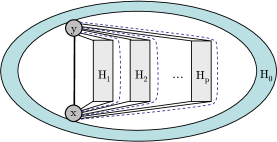
Figure 2: A separation pair $[x,y]$ and a separation of the inner components.

Lemma 3.1.

Let $\mathcal{E}(G)$ be a 1-planar embedding of a 1-planar graph $G$.

• The embedding $\mathcal{E}(G_{\boxplus})$ is triangulated.

• A pair of crossing edges is embedded as a kite or there is a W-configuration and a separation pair.

• $G_{\boxplus}$ has at most 4n-8 edges.

• $\mathcal{E}(G_{\boxplus})$ and $\mathcal{E}(G_{\boxplus}$ can be computed in linear time from $\mathcal{E}(G)$.

Proof.

The planar maximal embedding of each 3-connected component is triangulated [1]. It may change the embedding by rerouting an edge of a B-configuration, which thereby is turned into a kite, see Figs. 1 (b) and(c). Then the stated properties hold for $\mathcal{E}(G_{\boxtimes})$. At each separation pair $[x,y]$, the multi-edge between two components induces a triangulation with triangles consisting of $x,y$ and a crossing points of two edges incident to $x$ and $y$. After an elimination of all B-configurations there is a kite or a W-configuration for each pair of crossing edges.

Concerning the number of edges, at every separation pair $[x,y]$ with inner components $H_{1},\ldots,H_{p}$ and a 4-cycle $(a_{i},b_{i},c_{i},d_{i})$ as outer boundary of $H_{i}$ replace the pairs of crossing edges $\{x,c_{i}\},\{y,d_{i}\}$ and $\{x,a_{i+1}\},\{y,b_{i+1}\}$ by a kite with edges $\{c_{i},a_{i+1}\},\{c_{i},b_{i+1}\},\{d_{i},a_{i+1}\},\{d_{i},b_{i+1}\}$ and replace the i-th copy of $\{x,y\}$ between $H_{i}$ and $H_{i+1}$ by the edges $\{a_{i},a_{i+1}\}$ and $\{b_{i},b_{i+1}\}$ for $i=1,\ldots,p-1$. The resulting graph is 1-planar and has $q-1$ more edges than $G$. Hence, there are at most $4n-8$ edges. Each step from $\mathcal{E}(G)$ to $\mathcal{E}(G_{\boxplus})$ takes linear time and is performed on the embedding of the planarization.     $\sqcap$$\sqcup$

Concerning the density of 1-planar graphs, each W-configuration reduces the maximum number of edges by two, since each pair of edges crossing in the outer face can be substituted by four edges. This parallels the situation of planar graphs and 2-connected components.

Next, we consider vertex orderings of planar graphs which are later applied to graphs $G_{\square}$ and $G_{\bullet}$.

Let $\{s,t\}$ be an edge of a planar graph in the outer face of an embedding of $G$. An st-numbering is an ordering $v_{1},\ldots,v_{n}$ of the vertices of $G$ such that $s=v_{1}$, $t=v_{n}$ and every vertex $v_{i}$ other than $s$ and $t$ is adjacent to at least two vertices $v_{j}$ and $v_{k}$ with $j<i<k$. It is known that every 2-connected graph has st-numberings and an st-numbering can be constructed in linear time [29] for every edge $\{s,t\}$. An st-numbering induces an orientation of the edges of $G$ from a low ordered vertex to a high ordered one, called a bipolar orientation.

For convenience, we identify each vertex with its st-number and with its orthogonal polygon in a shape visibility representation and consider each edge as oriented. In simple words a vertex $u$ is less than vertex $v$ and vertex $v$ is placed at some point.

If $G$ is planar, then a bipolar orientation transforms $G$ into an upward planar graph and partitions the set of edges incident to a vertex $v$ into a sequence of incoming and a sequence of outgoing edges [21]. Accordingly, each vertex has two lists of faces below and above it, which are ordered clockwise or left to right. A face is below $v$ if both edges incident to $v$ are incoming edges, and above it, otherwise. In addition, at each separation pair $[x,y]$ with components $H_{0},\ldots,H_{k}$, the vertices of each inner component $H_{i}$ with $i\geq 1$ are ordered consecutively and they appear between $x$ and $y$ if $x<y$. We can write $x<H_{1}<\ldots<H_{k}<y$, where $H_{1},\ldots,H_{k}$ is any permutation of the inner components. For example, one may choose the cyclic ordering at $x$ if an embedding is given. st-numberings are a useful tool for the construction of visibility representations of planar graphs [21].

Canonical orderings are used for straight-line drawings of planar graphs. They were introduced by de Fraysseix et al. [19] for triangulated planar graphs and were generalized to 3-connected [35] and to 2-connected graphs [33]. The subsequent definition is taken from [6].

Definition 1.

Let $\Pi=(P_{0},\ldots,P_{q})$ be a partition of the set of vertices of a graph $G$ of size $n\geq 5$ into paths such that $P_{0}=\langle v_{1},v_{2}\rangle$, $P_{q}=\langle v_{n}\rangle$ and $\langle v_{1},P_{q},v_{2}\rangle$ is the outer face in clockwise order. For $k=0,\ldots,q$ let $G_{k}$ be the subgraph induced by $V_{k}=P_{0}\cup\ldots\cup P_{k}$ and let $C_{k}$ be the outer face of $G_{k}$, called contour. Then $\Pi$ is a canonical ordering if for each $k=1,\ldots,q-1$:

1. $C_{k}$ is a simple cycle.

2. Each vertex $z_{i}$ in $P_{k}$ has a neighbor in $V-V_{k}$.

3. $|P_{k}|=1$ or each vertex $z_{i}$ in $P_{k}$ has exactly two neighbors in $G_{k}$.

A canonical ordering $\Pi$ is refined into a vertex ordering $v_{1},\ldots,v_{n}$ by ordering the vertices in each $P_{k}$, $k>0$, straight or in reverse.

A canonical ordering can be computed by a peeling technique which successively removes the vertices of the paths in reverse order starting from $P_{q}$. For a quadrangle it would consist of two paths of length two. Care must be taken that the removal of the next path $P_{k}$ preserves the 2-connectivity of $G_{i}$ for $i=1,\ldots,k$, see [6, 35]. The contour $C_{k}$ is ordered left to right with $v_{1}$ at the left and $v_{2}$ at the right so that edge $\{v_{2},v_{1}\}$ closes the cycle.

A path $P$ is a feasible candidate for step $k+1$ of $\Pi=(P_{0},\ldots,P_{q})$ if also $(P_{0},\ldots,P_{k},P)$ can be extended to a canonical ordering of $G$.

Definition 2.

A canonical ordering $\Pi=(P_{0},\ldots,P_{q})$ is called leftish if for $k=0,\ldots,q-1$ the following is true: Let $c_{\ell}$ be the left neighbor of $P_{k+1}$ on $C_{k}$ and let $P$ be a feasible candidate for step $k+1$ with left neighbor $c_{\ell^{\prime}}$. Then $c_{\ell}<c_{\ell^{\prime}}$.

A leftish canonical ordering of a 3-connected planar graph can be computed in linear time [6]. For 2-connected planar graphs we extend the ordering as in the st-numbering case. At each separation pair $[x,y]$ with $x<y$ remove the inner components and compute the leftish canonical ordering of the 3-connected remainder. Then compute the leftish canonical ordering of each component and insert them just before $y$.

We study some properties of leftish canonical orderings on upward planar graphs. The orientation of the edges and upward direction is obtained from the (extended) leftish canonical ordering, which is an st-numbering with $s=1$ and $t=n$. Each edge has a face to its left and to its right if the graphs are 2-connected. Each face $f$ has a source and a sink, called $bottom(f)$ and $top(f)$, respectively. Suppose that edge $\{s,t\}$ is routed at the left. We call the face to the right of $\{s,t\}$ the leftmost face and the outer face is called the rightmost face [21].

In the remainder of this section, let $G$ be a 3-connected planar graph $G$ with an st-numbering whose faces are triangles or quadrangles that are traversed clockwise. The outer face is excluded.

Definition 3.

A quadrangle $f=(a,b,c,d)$ is called a rhomboid with bottom $a$, left end $b$, right end $d$, and top $c$ if there are two paths $\langle a,b,c\rangle$ and $\langle a,d,c\rangle$ enclosing $f$ with $b$ to the left of $f$ and $d$ to the right. Face $f$ is a left-trapezoid if there is an edge $\{a,d\}$ to the right of $f$ and a path $\langle a,b,c,d\rangle$ to the left. A right-trapezoid is defined accordingly, see Fig. 3.

(a)

(b)

(c)

Figure 3: (a) a rhomboid, (b) a left-trapezoid, and (c) a right-trapezoid

First, each path $P_{k}$ of a leftish canonical ordering $\Pi$ has length at most two, since one of $v_{1}$ and $v_{r}$ has at least two neighbors on $C_{k}$ if $P_{k}=\langle v_{1},\ldots,v_{r}\rangle$ with $r\geq 3$. Otherwise, there are faces as $m$-gons with $m>4$. If $P_{k}$ has length two, then it is inserted into $C_{k}$. Otherwise, $C_{k+1}$ is obtained by replacing a subsequence $\gamma$ of $C_{k}$ by $v$ with $P_{k}=\langle v\rangle$, where the vertices in $\gamma$ are covered by $v$ [19, 35].

Second, if $P_{k}=\langle v_{1},v_{2}\rangle$ is a path of length two, then the face below $P_{k}$ is a quadrangle $f_{k}=(u_{1},v_{1},v_{2},u_{2})$. We prefer rhomboids over trapezoids and therefore direct $P_{k}$ from $v_{2}$ to $v_{1}$ if $u_{2}=bottom(f_{k})$ and otherwise from $v_{1}$ to $v_{2}$. If $P_{k}=\langle v\rangle$ is a singleton then it may cover several faces, which are triangles, rhomboids, or trapezoids. We say that face $f_{k}$ is covered by $P_{k}$.

Third, we consider faces. For a vertex $v$ on a contour $C_{k}$ let $f_{1}(v),\ldots,f_{\nu}(v)$ be the left to right ordering of the faces incident to $v$ and above $C_{k}$ which is defined by the clockwise ordering of the outgoing edges. The outer face is discarded. For each quadrangle $f_{i}(v)=(v,b,c,d)$ let $t_{i}=top(f_{i}(v))$. Then $t_{i}=b$ if $f_{i}(v)$ is a right-trapezoid, $t_{i}=c$ if $f_{i}(v)$ is a rhomboid and $t_{i}=d$ if $f_{i}$ is a left-trapezoid and $t_{i}$ covers $f_{i}$. A face $f_{i}(v)=(v,b,d)$ or $f_{i}(v)=(v,b,c,d)$ for $i=1,\ldots,\nu$ has left-support if there is a contour $C_{\ell}=(1,\ldots,b,v,\ldots,2)$ and right-support if $C_{\ell}=(1,\ldots,v,d,\ldots,2)$. If $f_{i}(v)$ has left-support and $d$ is in $P_{k+j_{i}}$ for some $i_{j}\geq 1$ then either $d$ is immediately to the left of $v$ on the contour $C_{k+j_{i}}$ or the placement of $d$ covers $v$. The case is symmetric to the right if $f_{i}(v)$ has right support.

For an illustration see Fig. 4.

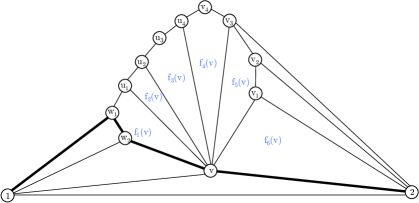
Figure 4: A sequence of faces above vertex $v$. Starting from a contour $C_{k}=(1,w_{1},w_{2},v,2)$ there is a leftish canonical ordering $\Pi=(\langle u_{1}\rangle,\langle u_{2}\rangle,\langle u_{3},u_{4}\rangle,\langle v_{1}\rangle,\langle v_{2}\rangle,\langle v_{3}\rangle,\langle v_{4}\rangle)$. Face $f_{1}(v)$ is a left-trapezoid, $f_{2}(v)$ and $f_{6}(v)$ are triangles, $f_{4}(v)$ is a rhomboid, and $f_{5}(v)$ is a right-trapezoid. Face $f_{2}(v)$ is a rhomboid if edge $\{u_{3},u_{4}\}$ is oriented from $v_{4}$ to $v_{3}$ and a left-trapezoid, otherwise. Face $f_{1}(v)$ has left-support, $f_{5}(v)$ has right-support, and $f_{4}(v)$ has left- and right-support. The sequence $(u_{1},u_{2},u_{3},u_{4},v_{4},v_{3},v_{2},v_{1})$ of neighbors of $v$ above $C_{k}$ is bitonic.

Lemma 3.2.

Let $v$ be a vertex on a contour $C_{k}$. A quadrangle $f$ with $v=bottom(f)$ has left-support (right-support) if $f$ is a left-trapezoid (right-trapezoid).

Proof.

For a contradiction, suppose that $f=(a,b,c,d)$ is a left-trapezoid and has no left-support. Since $f$ is a left-trapezoid, vertex $b$ appears before vertices $c$ and $d$ in the vertex ordering. If $b$ has a neighbor to the right of $v$ on the contour, then $f$ cannot be a left-trapezoid.     $\sqcap$$\sqcup$

Note that the statement may not apply to the outer face, which later on may need a spacial treatment. The type of quadrangles $f(v)$ is determined by their support and the length of the path with the top vertex in the leftish canonical ordering.

Let $f_{1}(v),\ldots,f_{\nu}(v)$ be the left to right (clockwise) ordering of faces with bottom $v$ above $C_{k}$ and let $j_{1}<\ldots<j_{\mu}$ be the subsequence of quadrangles. The other faces are triangles. For $i=1,\ldots,\nu$ let $P_{t_{i}}$ contain the top vertex of $f_{i}$ so that $f_{i}$ is closed by $P_{t_{i}}$. Thus, $t_{i}$ is the time stamp for the completion of face $f_{j_{i}}$ in a canonical ordering and a drawing based on it.

Lemma 3.3.

If a face $f=f_{i}(v)$ for $i=1,\ldots,\nu$ is a triangle, then it has left-support or right-support and $P_{t_{i}}$ is a singleton. If $f$ is a quadrangle, then $f$ is a left-trapezoid if $f$ has no right-support and $P_{t_{i}}$ is a singleton. Face $f$ is a right-trapezoid if $f$ has no left-support and $P_{t_{i}}$ is a singleton, and $f$ is a rhomboid if $f$ has left and right-support or $P_{t_{i}}$ is a path of length two.

Proof.

If $f$ is a triangle, then it must be closed by a path of length one of the leftish canonical ordering and therefore it has left- or right-support.

Each quadrangle $f$ has a left- or a right-support, since the paths have length at most two. If $f$ has no right-support and $P_{t_{i}}$ is a singleton, then vertices $b$ and $c$ are placed before vertex $d=top(f)$ if $f=(v,b,c,d)$ in clockwise order and $f$ is a left-trapezoid. The case to the right is symmetric. If $f=(v,b,c,d)$ has left- and right-support, then $c=top(f)$ and $b$ and $d$ are less than $c$ in the vertex numbering, so that $f$ is a rhomboid. If $P_{t_{i}}$ is a path of length two, then $f$ is a rhomboid by construction.     $\sqcap$$\sqcup$

The leftish canonical ordering also determines the order in which the vertices of the faces at $v$ are placed.

Lemma 3.4.

For a leftish canonical ordering $\Pi$ and a vertex $v$ on a contour $C_{k}$, the clockwise sequence of neighbors $w_{1},\ldots,w_{z}$ of $v$ above $C_{k}$ is bitonic, i.e., there is some $m$ with $1\leq m\leq z$ such that $w_{1}<\ldots<w_{m}$, $w_{m+1}>\ldots>w_{z}$ and $w_{m}<w_{z}$ in $\Pi$.

For an illustration, see Fig. 4 and observe that the sequence of the vertices corresponds to the order in which the faces above $v$ are completed, first from left to right and then from right to left.

Proof.

Consider the clockwise sequence of faces $f_{1}(v),\ldots,f_{\eta}(v)$ with $\eta\leq z$. Then there is some $\mu$ so that $f_{j}$ has left-support for $i=1,\ldots,\mu$ and $f_{j}$ has right-support for $\mu+1,\ldots,\eta$. Otherwise, suppose for some $\kappa$ with $1\leq\kappa<\mu-1$ face $f_{\kappa}$ has right-support and face $f_{\kappa+1}$ has left-support. Then $C_{j_{\kappa}}=(1,\ldots,v,d,\ldots,2)$ for some vertex $d$ of $f_{\kappa}$ and $C_{j_{\kappa+1}}=(1,\ldots,d,v,\ldots,2)$, a contradiction.

In consequence, for $1\leq j<\mu$ and vertices $x$ in $f_{j}(v)$ and $y$ in $f_{j+1}(v)$ it holds that $x<y$ in $\Pi$. Similarly, we have $x>y$ for vertices $x$ in $f_{j}(v)$ and $y$ in $f_{j+1}(v)$ and $\mu+1\leq j\leq z$. Paths of length two of $\Pi$ are ordered in accordance with this ordering. Now let $w_{1},\ldots,w_{m}$ be the vertices in faces $f_{1}(v),\ldots,f_{\mu}(v)$. By planarity, the ordering of the faces is in accordance with the ordering of the vertices in $\Pi$, which is bitonic.     $\sqcap$$\sqcup$

Note that the sequence of neighbors of $v$ is not continuous in the leftish canonical ordering. In general, a neighbor $w_{i}$ of vertex $v$ on $C_{k}$ is a right-support of some face $f(u)$ for a vertex $u$ to the left of $v$ on $C_{k}$.

4 Rectangle Visibility Representation of IC-planar Graphs

The proofs of Theorems 1 and 2 are constructive. The outline of the algorithms is as follows: Take an embedding $\mathcal{E}(G)$ as a witness for IC-planarity and 1-planarity, respectively. The embedding is first augmented to $\mathcal{E}(G_{\boxplus})$ as given in Lemma 3.1. Since planar maximal IC-planar graphs are 3-connected we can use $\mathcal{E}(G_{\boxtimes})$ in this case. Thereby, some edges can be rerouted and some are multiplied to separate components. If the input were a graph, then constructing the normal form embedding is an NP-hard problem, since the general recognition problem is NP-hard and is solvable in polynomial time for graphs with a normal form embedding [13, 18]. Next, $G_{\boxplus}$ is planarized to $G_{\square}$ by a removal of all pairs of crossing edges while preserving the (new) embedding. The planarization is obtained via $G_{\bullet}$ for IC-planar graphs. In a nutshell, the algorithms use a standard algorithm for the construction of a visibility representation of a planar graph, see [21, 36, 42, 46]. Finally, the pairs of crossing edges are added to the planar visibility representation of $G_{\square}$. In case of IC-planar graphs, there is a quadrangle $f=(a,b,c,d)$ which is drawn as a rhomboid with a vertex $b$ to the left and a vertex $d$ to the right of $f$ and at the same level ($y$-coordinate) into which a pair of crossing edges is inserted. In the second case, we use a leftish canonical ordering for an st-numbering and the capabilities of horizontal and vertical lines of sight in the weak visibility version.

First, we define kite-contraction and kite-expansion operations on IC-planar embeddings in normal form. By IC-planarity, two kites have no common vertex and do not intersect so that kite-contractions do not interfere. Moreover, each pair of crossing edges is embedded as a kite and $G$ is 3-connected if $\mathcal{E}(G)$ is an IC-planar embedding in normal form,[1, 5]

Definition 4.

Let $\mathcal{E}(G)$ be an IC-planar embedding in normal form and suppose there is an $st$-ordering of $G$.

A kite-contraction contracts a kite $\kappa$ with boundary $(a,b,c,d)$ of $\mathcal{E}(G)$ to a single vertex $v_{\kappa}$ so that $v_{\kappa}$ inherits all incident edges and henceforth has multi-edges. A kite-expansion is the inverse operation on the boundary and replaces $v_{\kappa}$ by the 4-cycle $(a,b,c,d)$. Both operations are adjacency preserving so that a kite-contraction followed by a kite-expansion just removes the pair of crossing edges of $\kappa$.

The kite-contraction $G_{\bullet}$ of $G$ is obtained by contracting all kites of $\mathcal{E}(G)$.

Lemma 4.1.

Let $\mathcal{E}(G)$ be an IC-planar embedding in normal form. Then graph $G_{\bullet}$ is a 3-connected planar graph, which can be computed from $\mathcal{E}(G)$ in linear time.

Proof.

For planarity, first remove one edge from each pair of crossing edges of each kite, which results in a graph $G_{\triangle}$. Then $G_{\triangle}$ is a triangulated planar graph that inherits its embedding from $\mathcal{E}(G)$. Thus it is 3-connected. Next contract the edges that remain from each kite to a vertex $v_{\kappa}$. Since the planar graphs are closed under taking minors, the edge contractions preserve planarity and yield $G_{\bullet}$, since by IC-planarity each vertex $v$ either remains or is contracted to a vertex $v_{\kappa}$. The removal of multi-edges results in a triangulated planar graph, which is 3-connected, and so is $G_{\bullet}$.

It takes linear time to obtain $G_{\triangle}$ from $\mathcal{E}(G)$ and $G_{\bullet}$ from $G_{\triangle}$.     $\sqcap$$\sqcup$

Note that this type of kite-contractions cannot be applied to 1-planar (or NIC-planar) graphs, since vertices may belong to several kites. Instead one may contract a kite to a single vertex which corresponds to its crossing point or consider the $K_{4}$ network [16].

Next, we consider rhomboidal st-numberings.

Definition 5.

An embedding $\mathcal{E}(G)$ of a 1-planar graph in normal form is called rhomboidal with respect to an st-numbering if the $K_{4}$ subgraph induced by a pair of crossing edges is embedded as a kite whose boundary is a rhomboid.

Rhomboidal embeddings distinguish IC-planar graphs from NIC-planar graphs.

Lemma 4.2.

For every IC-planar graph $G$ and every planar edge $\{s,t\}$ there is a rhomboidal embedding which can be computed in linear time from $\mathcal{E}(G)$.

Proof.

First, construct an IC-planar embedding in normal form with $\{s,t\}$ in the outer face. Next, compute a kite-contraction $\mathcal{E}(G_{\bullet})$ and an st-numbering of $G_{\bullet}$. Then do the kite-expansion and extend the st-numbering of $G_{\bullet}$ to an st-numbering of $G$ as follows: For each contracted kite $\kappa$ determine a top and a bottom vertex and then the left and right ends of the face $f$ of $\kappa$ without the pair of crossing edges. Expand $\kappa$ in $\mathcal{E}(G_{\bullet})$. If there is exactly one vertex $u$ of $\kappa$ with only incoming (multi-)edges, then let $u=bottom(f)$. Choose the top vertex opposite to $u$, and the left and right ends to the left and right of $f$. Similarly, choose $v=top(f)$ if only $v$ has outgoing (multi-)edges and choose $bottom(f)$ opposite to $v$. Otherwise, choose a pair of opposite vertices so that $u=bottom(f)$ has incoming and $v=top(f)$ has outgoing (multi-)edges and determine the left and right ends.

Clearly, each step takes linear time.     $\sqcap$$\sqcup$

We are now able to describe 1-planar graphs that admit a right angle crossing drawing which is a step towards the intersection of 1-planar and RAC graph that is asked for in [15, 26].

Theorem 3.

If $G$ is a 3-connected 1-planar graph so that the augmentation $G_{\boxtimes}$ has a rhomboidal embedding with respect to a canonical ordering, then $G$ is a RAC graph.

Proof.

Our algorithm is a simplification of the technique used in Case 1 of the proof of Theorem 2 in [15], where more details can be found.

The planar subgraph $G_{\square}$ of $G_{\boxtimes}$ is 3-connected [1] and has a rhomboidal canonical ordering by assumption. Graph $G_{\square}$ is processed according to the canonical ordering using the shift technique as in [19] and extended to 3-connected graphs in [35]. For every quadrilateral face $f=(a,b,c,d)$ in clockwise order with $a=bottom(f)$ and $c=top(f)$, the algorithm first places $a$, then $b$ and $d$ in any order, and finally $d$ according to the canonical ordering. Vertex $b$ is placed on the $-1$-diagonal through $a$ to the left and $d$ is placed on the $+1$-diagonal through $a$ to the right and at the intersection with the $+1$ and $-1$ diagonal of the left lower and right lower neighbors, respectively. The technique in [15] is a leveling of $b$ and $d$. If $b$ is placed $\delta$ units below $d$, or vice versa, then lift $b$ to the level of $d$ by $2\delta$ extra shifts to the left. If $b$ has been leveled with other vertices, then the shift is synchronously applied to all vertices that are leveled with $b$. Alternatively, on may apply the critical (or longest) path method so that the critical paths to $b$ and $d$ have the same length. At the placement of $c=top(f)$ we shift $b$ to the left or $d$ to the right so that $c$ is placed vertically above $d$. Then edge $\{b,d\}$ is inserted as a horizontal line and $\{a,c\}$ as a vertical one. Later on, $b,a$ and $d$ are shifted by the same amount as $c$, so that the right angle crossing of $\{b,d\}$ and $\{a,c\}$ is preserved.     $\sqcap$$\sqcup$

There are rhomboidal 1-planar graphs that are not NIC-planar, such as $k\times k$ grids with a pair of crossing edges in each inner quadrangle and a triangulation of the outer face. (The graphs are not NIC-planar, because they have too many edges). On the other hand, every IC-planar graph admits a rhomboidal embedding and we have a simpler proof than in [15].

Corollary 1.

Every IC-planar graph is a RAC graph.

Corollary 2.

There are 3-connected 1-planar graphs and NIC graphs that do not admit a rhomboidal canonical ordering.

Proof.

There are 1-planar graphs [24] and even NIC-planar graphs [5] that are not RAC and a rhomboidal canonical ordering would contradict Theorem 3.     $\sqcap$$\sqcup$

We now turn to rectangle visibility representations of IC-planar graphs and the proof of Theorem 1.

A visibility representation of a 2-connected planar graph $G$ is commonly obtained by the following steps [21, 36], which we call VISIBILITY-DRAWER:

1. Compute an st-numbering $\delta(v)$ for the vertices of $G$ with an edge $\{s,t\}$ and $\delta(s)=1$ and $\delta(t)=n$. Embed edge $\{s,t\}$ at the left and orient the edges according to the st-numbering.

2. Compute the $s^{*}t^{*}$-numbering of the dual graph $G^{*}$ where $s^{*}$ is the face to the right of $\{s,t\}$ and $t^{*}$ is the outer face.

3. For an oriented edge $e$ let left$(e)$ (right$(e)$) be the $s^{*}t^{*}$-number of the face to the left (right) of $e$. For a vertex $v\neq s,t$ let left$(v)=$ min$\{$left$(e)\,|\,e$ is incident to $v\}$ and right$(v)=$ max$\{$right$(e)\,|\,e$ is incident to $v\}$.

4. For each vertex $v\neq s,t$ draw a bar between $(\textrm{left}(v),\delta(v))$ and $(\textrm{right}(v)-1,\delta(v))$ and draw a bar between $(0,0)$ and $(M-1,0)$ for $s$ and between $(0,n-1)$ and $(M-1,n-1)$ for $t$ where $M\leq 2n-4$ is the number of faces of $G$.

5. Draw each edge $e=\{u,v\}\neq\{s,t\}$ between $(\textrm{left}(e),\delta(u))$ and $(\textrm{left}(e),\delta(v))$ and draw $\{s,t\}$ at $x=1$.

There is exactly one vertex at each level $y=1,\ldots,n$ if the st-numbers are used for the $y$-coordinates of the vertices. More compact drawings are obtained by using the critical path method or topological sorting [21, 36]. The drawings are not really pleasing, since many lines of sight are at the ends of the bars. There are no degenerated faces since the right end of a bar to the left of face $f$ is at least one unit to the left and of a bar to the right of $f$. The drawing algorithm preserves the given embedding.

The change of the embedding at B-configurations can be undone by modifying the computation of the $x$-coordinates of the lines of sight. Before the computation of the dual $s^{*}t^{*}$-numbering add a copy of the rerouted $\{s,t\}$ edge at its original place and remove the edge(s) that were added for the 3-connectivity and compute $\delta^{*}$ on the new embedding. The line of sight for the edge $\{s,t\}$ can be drawn at several places [12] and we must choose the one that preserves the embedding.

1

Input: An IC-planar embedding $\mathcal{E}(G)$.

2

Output: A rectangle visibility representation $\mathcal{RV}(G)$.

3

4Transform $\mathcal{E}(G)$ into a normal form embedding $\mathcal{E}(G_{\boxtimes})$.

5 Compute the planar graph $G_{\square}$ and a rhomboidal st-numbering $\delta$ of $G_{\square}$.

6 Compute an $s^{*}t^{*}$-numbering $\delta^{*}$ of the dual graph $G_{\square}^{*}$.

7 foreach vertex v of $G_{\square}$ do

8       if $v$ is the left (right) end of a rhomboid and $u$ is the other end then

9            $d(v)=\delta(u)+\delta(v)$

10       else

11             $d(v)=2\delta(v)$

12      

13 Compute a planar visibility representation of $G_{\square}$ by

14  VISIBILITY-DRAWER with vertices on level $d(v)$ and edges at left$(e)$. foreach pair of crossing edges $\{a,c\}$ and $\{b,d\}$ in a

15  rhomboid $f=(a,b,c,d)$ with $d(a)<d(b)=d(d)<d(c)$ do

16       Add a horizontal line of sight at level $d(b)$ between the bars of $b$ and $d$.

17       Add a vertical line line of sight at $\delta^{*}(f)+0.5$ between

18        the bars of $a$ and $c$.

19 Scale all $x$-coordinates by two.

Remove (or ignore) all lines of sight of edges not in $G$.

Algorithm 1 IC-RV-DRAWER

The following Lemma concludes the proof of Theorem 1.

Lemma 4.3.

Algorithm IC-RV-DRAWER constructs a rectangle visibility representation of an IC-planar graph on $O(n^{2})$ area and operates in linear time.

Proof.

The algorithm computes a planar visibility representation of $G_{\square}$ in linear time as proved in [21, 42, 46] on an area of size $(2n-5)\times 2n$, which is scaled by a factor of two in $x$-dimension.

Each pair of crossing edges is in a kite of $G_{\boxtimes}$ whose boundary is embedded as a rhombus $f=(a,b,c,d)$ with $a=bottom(f)$. Then the y-coordinates of $b$ and $d$ coincide and $d$ is a weighted topological sorting as used in [21]. There is a gap of one unit between the bars of $b$ and $d$, since the bar of $b$ ends at $\delta^{*}(f)-1$ and the bar of $d$ begins at $\delta^{*}(f)$. Now, edges $\{a,c\}$ and $\{b,d\}$ are added so that they cross inside $f$.

Since $G$ has at most $13/4n-4$ edges, the transformation into normal form takes linear time so that $G_{\boxtimes}$ and $G_{\square}$ have size $O(n)$. The visibility representation of $G_{\square}$ is computed in linear time [21]. There are at most $n/4$ pairs of crossing edges which are each inserted in $O(1)$ time.     $\sqcap$$\sqcup$

5 T-Visibility of 1-planar Graphs

For the T-visibility representation of 1-planar graphs we use a leftish canonical ordering as an st-numbering and draw $G_{\square}$ by VISIBILITY-DRAWER. Note that $G_{\square}$ may have multi-edges at separation pairs, which each introduces a face. In total, $G_{\square}$ has at most $2n-4$ faces, since each multi-edge could be substituted by a planar edge. For the pairs of crossing edges we expand some vertices to a $\bot$-shape. A $\bot$-shaped vertex consists of a horizontal bar and a vertical pylon. By a horizontal flip we obtain a T-shape visibility representation. If vertex $v$ is $\bot$-shaped, then the pylon is inserted into the face of a left- or right-trapezoid $f$ with $v=bottom(f)$ and $top(f)$ is maximum. For each quadrangle $f=(v,b,c,d)$, the edges $\{v,c\}$ and $\{b,d\}$ were removed in the planarization step. They are reinserted as follows: If $f$ is a rhomboid, then the lower of $b$ and $d$ gets a pylon for an $\llcorner$- or $\lrcorner$-shape so that $\{b,d\}$ is a horizontal line that is crossed by a vertical line of sight for $\{a,c\}$ inside $f$. If $f$ is a left-trapezoid, then the bar of $b$ is extended to the right and edge $\{b,d\}$ is added as a vertical line of sight inside $f$. Accordingly, extend the bar of $d$ to the left if $f$ is a right-trapezoid. The particularity is the drawing of edge $\{v,c\}$ as a horizontal line of sight from the pylon of $v$ to the bar (or pylon) of $c$, as depicted in Fig. 5. This line of sight is unobstructed, since there is exactly one bar on each level by the use of $st$-numbers for the $y$-coordinate of the vertices and there is no obstructing pylon from another vertex by the use of the leftish canonical ordering and the bitonic order of the vertices above a vertex $v$, as stated in Lemma 3.4.

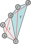
(a)

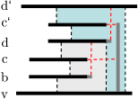
(b)

Figure 5: (a) Two left-trapezoids $f=(v,b,c,d)$ and $f^{\prime}=(v,d,c^{\prime},d^{\prime})$ and (b) their visibility representation.

There is a special case at separation pairs and W-configurations, see Fig. 6. If $G-\{x,y\}$ partitions into an outer component $H_{0}$ and inner components $H_{1},\ldots,H_{p}$, then VISIBILITY-DRAWER places the inner components from left to right between the bars of $x$ and $y$ and separates them in $x$-dimension by the $st$-numbering and in $y$-dimension by the $s^{*}t^{*}$-numbering. It admits a representation of the copies of edge $\{x,y\}$ by vertical lines of sight.

Consider the planarization $\widehat{H}_{\square}$ of an inner component $H$ together with the separation pair $x,y$. The outer face of $\widehat{H}_{\square}$ is a quadrangle $f=(x,b,c,y)$ which is embedded as a left-trapezoid with a copy of $\{x,y\}$ on the right. The vertex numbering from the leftish canonical ordering is $x<b<w<c<y$, where $w\neq b,c$ is any other vertex of $H_{i}$. Thus, $b$ and $c$ are the first and last vertex of $H_{i}$. They are not unique, since the embedding of $H_{i}$ can be flipped. In particular, $P_{q-1}=\langle c\rangle$ and $P_{q}=\langle t\rangle$ are the last two paths in the leftish canonical ordering of $\widehat{H}_{\square}$, since there is no separating triangle $\Delta=(t,c,w)$ for some vertex of $H$. Hence, $b$ and $c$ are placed on the lowest and highest levels of the vertices of $H$. The outer edge $\{b,t\}$ is represented as a vertical line of sight between the bars of $b$ and $t$ as if it were a planar edge, whereas edge $\{x,c\}$ is a horizontal line of sight from the pylon of $x$ to the pylon of $c$. Algorithm T-DRAWER constructs the visibility representation.

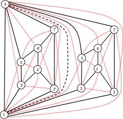
Figure 6: A graph $DXW$ consisting of two copies of the extended wheel graph $XW_{6}$ with vertices $1,\ldots,8$ and $1,2^{\prime},\ldots,7^{\prime},8$. Planar edges are drawn black and bold and crossing edges red and dotted. The copy of edge $\{1,8\}$ is drawn dashed. The extended leftish canonical ordering is $\Pi=(\langle 1,2\rangle,\langle 3,4\rangle,\langle 5,6\rangle,\langle 7\rangle,\langle(1),2^{\prime}\rangle,\langle 3^{\prime},4^{\prime}\rangle,\langle 5^{\prime},6^{\prime}\rangle,\langle 7^{\prime}\rangle,\langle 8\rangle)$.

1

Input: A 1-planar embedding $\mathcal{E}(G)$.

2

Output: A T-visibility representation $\mathcal{TVR}(G)$.

3

4Compute $\mathcal{E}(G_{\boxplus})$ from $\mathcal{E}(G)$.

5

6Compute $G_{\square}$ from $\mathcal{E}(G_{\boxplus})$ by removing all pairs of crossing edges.

7

8Compute an $st$-numbering $\delta$ of $G_{\square}$ as an extension of a leftish canonical

9  ordering of each 3-connected component.

10 Compute the $s^{*}t^{*}$-numbering $\delta^{*}$ of the dual graph $G_{\square}^{*}$.

11

12Compute the planar visibility representation of $G_{\square}$ by

13  VISIBILITY-DRAWER.

14

15foreach vertex $v$ with quadrangles $f$ such that $v=bottom(f)$ do

16       int $v_{max}=0$; face $f_{max}$

17       foreach left-trapezoid $f=(v,b,c,d)$ do

18             if $v_{max}<c$ then

19                   $v_{max}=c$;   $f_{max}=f$

20             Extend the bar of $b$ by $1/3$ to the right and at its right end

21             add a vertical line of sight for $\{b,d\}$.

22       foreach right-trapezoid $f=(v,d,c,b)$ do

23             if $v_{max}<c$ then

24                   $v_{max}=c$;   $f_{max}=f$

25             Extend the bar of $b$ by $1/3$ to the left and at its left end

26             add a vertical line of sight for $\{b,d\}$.

27       foreach rhombus $f=(v,b,c,d)$ do

28             Enlarge the bar of the lower of $b$ and $d$ by a pylon at an end

29              and inside $f$ and up to the bar of the upper vertex.

30             Add a horizontal line of sight for $\{b,d\}$ at the top of the pylon.

31             Add a vertical line of sight for $\{v,c\}$ between the bars of $v$ and $c$

32              at $\delta^{*}(f)+1/3$

33            

34      

35      if $v_{max}\neq 0$ then

36             Enlarge the bar of $v$ by a pylon inside $f_{max}(v)$ from

37              $(\delta^{*}(f_{max}(v))+1/3,\delta(v))$ to $(\delta^{*}(f_{max}(v))+1/3,\delta(v_{\max}))$

38             foreach trapezoid $f=(v,b,c,d)$ do

39                  if $f$ is not a left-trapezoid with a separation pair $[v,d]$ then

40                         Add a horizontal line of sight for $\{v,c\}$

41                          from the pylon to the bar of $c$.

42                   else  // the horizontal line of sight may be occupied

43                         Enlarge the bar of $c$ by a pylon of height $1/2$.

44                         Add a horizontal line of sight for $\{v,c\}$ at the top of the pylon of $c$.

45                  

46            

47      

48 Scale all $x$-coordinates by three and all y-coordinates by two.

Algorithm 2 T-DRAWER

Lemma 5.1.

Suppose $G$ is a 3-connected 1-planar graph and there is no W-configuration in the outer face of an embedding of $G$. For a vertex $v$ on a contour $C_{k}$, let $f_{j_{1}}(v),\ldots,f_{j_{\mu}(v)}$ be the sequence of left- and right-trapezoids above $v$ from left to right with $f_{i}(v)=(v,b_{i},c_{i},d_{i})$. Let $v_{max}=\max\{c_{i}\,|\,i=j_{1},\ldots,j_{\mu}\}$ and let $f_{max}(v)$ be the trapezoid containing $v_{max}$.

Then the pylon of $v$ inside $f_{max}(v)$ can see the bar of each vertex $c_{i}$ for $i\in\{j_{1},\ldots,j_{\mu}\}$.

Proof.

By Lemma 3.4, there is a bitonic sequence of clockwise neighbors of $v$, which each has is own $y$-coordinate according to the leftish canonical ordering. Hence, a horizontal line of sight from the pylon of $v$ is unobstructed by bars of other vertices. A horizontal line of sight from the pylon to $c_{i}$ intersects only vertical lines of sight of planar edges $\{v,w\}$ with $c_{i}<w$ and $c_{i}$ and $w$ are on the same side of the pylon, i.e., $c_{i},w<w_{m}$ or $c_{i},w>w_{m}$, where $w_{m}$ is the maximum neighbor of $v$ (or the top vertex of $f_{j_{\mu}}(v)$) in the leftish canonical ordering. Hence, a line of sight $\{v,c_{i}\}$ is unobstructed by pylons of other vertices. In consequence, each edge $\{v,c_{i}\}$ with $i\in\{j_{1},\ldots,j_{\mu}\}$ is represented in the visibility representation constructed by T-DRAWER.     $\sqcap$$\sqcup$

Finally, consider a separation pair $[x,y]$ with inner components $H_{1},\ldots,H_{p}$. The st-numbering extending the leftish canonical ordering of 3-connected components inserts the vertices of each component consecutively and just before $y$ so that there is a subsequence $x,H_{0}^{\prime},H_{1},\ldots,H_{p},y$, where $H_{0}^{\prime}$ is a subgraph of the outer component that is added by the leftish canonical ordering between $x$ and $y$. Each component $H_{i}$ is drawn in a box $B(H_{i})$ and the boxes are ordered monotonically in $x$- and in $y$-dimension to a staircase between the bars of $x$ and $y$ both by the common visibility drawer and by T-DRAWER, as illustrated in Fig. 7.

Consider the outer face of an inner component including the separation pair. Without crossing edges, there is a quadrangle $f_{out}(H)=(x,b,c,y)$, which is embedded as a left-trapezoid. However, $f_{out}(H)$ has no left-support, since $x<b<c<y$ in the leftish canonical ordering and edge $\{x,y\}$ of $f_{out}(H)$ is a copy of the original edge. This case is treated as an exception. Edge $\{b,y\}$ is drawn inside $f_{out}(H)$ and to the right of $H$ after an extension of the bar of $b$ to the right. Vertex $x$ is $\bot$-shaped with a high pylon up to $y$ which is placed in the face to the right of the original edge $\{x,y\}$. The pylon can see all vertices that are neighbors of $x$ in the trapezoids of $H$ by Lemma 5.1. However, the horizontal line of sight to $c$ may be occupied, as in Fig. 8. Fortunately, $c$ is the last vertex of $H$ in the leftish canonical ordering and a short pylon for the bar of $c$ admits a horizontal line of sight between $x$ and $c$. Since the inner components are separated in $y$-dimension, the pylon of $x$ can see all neighbor of $x$ in the trapezoids of the inner components.

The following Lemma concludes the proof of Theorem 2.

Lemma 5.2.

Algorithm T-DRAWER constructs a T-visibility representation of a 1-planar graph on $O(n^{2})$ area and operates in linear time.

Proof.

The computations of $G_{\boxplus}$, the removal of all pairs of crossing edges for $G_{\square}$, the st-numbering as an extension of a leftish canonical ordering, the $s^{*}t^{*}$-numbering and the planar visibility representation of $G_{\square}$ each take linear time if a 1-planar embedding of $G$ is given. There are at most n-2 pairs of crossing edges which can each be inserted in $O(1)$ time into the visibility representation of $G_{\square}$. Hence, T-DRAWER runs in liner time. The visibility representation of $G_{\square}$ has size at most $(2n-5)\times n$, which is expanded by a factor of six.

The common visibility drawer provides a correct visibility representation of $G_{\square}$. For each 3-connected component without a W-configuration, the pairs of crossing edges are correctly added to the visibility representation by Lemma 5.1. The pair of edges crossing in the outer face of a W-configuration is visible by the special treatment in lines 34 and 35. Since inner components at a separation pair $[x,y]$ are strictly separated in both dimensions and are placed between the bars (shapes) of $x$ and $y$, there is a line of sight between the shapes of $x$ and $y$ for each edge between $x$, $y$ and vertices of inner components. Finally, consider the decomposition tree. If $H$ is an inner component at a separation pair $[x,y]$, then there is no edge $\{u,v\}$ from a vertex $u$ with $x\neq u\neq y$ of the outer component to a vertex $v$ of $H$ and, hence, there is no need for a line of sight. In addition, there is no need for a horizontal line of sight from a pylon through the visibility representation of an inner component, since the st-numbering groups components recursively and thereby separates them. Hence, the pylons in inner components do not obstruct horizontal lines of sight from pylons of vertices of the outer component.     $\sqcap$$\sqcup$

It is important to use weak visibility, since a pylon can see the bars and pylons of many other vertices, which is forbidden in the strong visibility version.

As an example, consider the extended wheel graph $XW_{6}$ [43] and then take copies of it and identify two vertices, here 1 and 8. These graphs have been used for the construction of sparse maximal 1-planar graphs [16] and for a linear lower bound on the number of legs (vertex complexity) in embedding-preserving caterpillar-shape visibility representations [23]. Graph $XW_{6}$ can be seen as a cube in 3D in which each face contains a pair of crossing edges.

The visibility representation of $G_{\square}$ from the common visibility drawer is displayed in Fig. 7 and the $\bot$-shape visibility representation of T-DRAWER in Fig. 8. Note that the graphs even admit a rectangle visibility representation (use the high pylons of vertices $1,2,5,2^{\prime},5^{\prime}$ and fill $4$ and $4^{\prime}$ to a rectangle in Fig. 8).

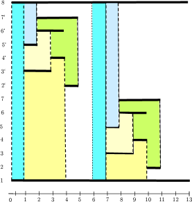
Figure 7: A visibility representation of $DXW_{\square}$ from Fig. 6 with dashed lines of sight and colored faces.

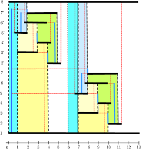
Figure 8: The T-shaped visibility representation of graph $DXW$ from Fig. 6 by T-DRAWER (with pylons in blue).

6 General Shape Visibility Graphs

There is a natural ordering relation $\sigma<\sigma^{\prime}$ between shapes if $\sigma$ is a restriction of $\sigma^{\prime}$ including rotation and flip. For example, $\textsf{I}<\textsf{L}<\textsf{F}<\textsf{E}$ and $\textsf{I}<\textsf{T}<\textsf{E}<rake<caterpillar$. Clearly, every $\sigma$-shape visibility graph is a $\sigma^{\prime}$-shape visibility graph if $\sigma<\sigma^{\prime}$. However, it is unclear whether different shapes imply different classes of shape visibility graphs. Moreover, shapes with cycles, such as O or B are not really useful for shape visibility representations, since a cycle corresponds to an articulation vertex.

For shape visibility graphs we can state:

Lemma 6.1.

Every shape visibility graph has thickness two.

Proof.

The subgraph induced by the horizontal (vertical) lines of sight is planar.     $\sqcap$$\sqcup$

Corollary 3.

$\sigma$-visibility graphs of size $n$ have at most $6n-12$ edges and there are $\sigma$-visibility graphs with $6n-20$ edges for every shape $\sigma$.

The upper bound follows from Lemma 6.1 and the lower bound has been proved by Hutchinson et al. [34] for rectangle visibility graphs. The exact bound are unclear for all shapes except rectangles.

The extended wheel graph $XW_{6}$ even admits a rectangle visibility representation, and so do all wheel graphs $XW_{2k}$ with $k\geq 3$. An extended wheel graph consists of a cycle of vertices $v_{1},\ldots,v_{2k}$ of vertices of degree six so that each $v_{i}$ is adjacent to its next and next but one vertex in cyclic order. In addition, there are two poles $p$ and $q$ that are adjacent to all $v_{i}$ (but there is no edge $\{p,q\})$. Extended wheel graphs play a prominent role for 1-planar graphs with $4n-8$ edges [14, 43, 45].

We close with some open problems:

Conjecture:

1. Every 1-planar graph with $4n-8$ edges is a rectangle visibility graph.

2. There are L-visibility graphs that are not rectangle visibility graphs (I-shape) and there are T-visibility graphs that are not L-visibility graphs.

7 Acknowledgement

I wish to thank Christian Bachmaier for his useful comments and suggestions.

References

- [1] M. J. Alam, F. J. Brandenburg, and S. G. Kobourov. Straight-line drawings of 3-connected 1-planar graphs. In S. Wismath and A. Wolff, editors, GD 2013, volume 8242 of LNCS, pages 83–94. Springer, 2013.
- [2] M. Albertson. Chromatic number, independence ratio, and crossing number. Ars Math. Contemp., 1(1):1–6, 2008.
- [3] T. Andreae. Some results on visibility graphs. Discrete Applied Mathematics, 40(1):5–17, 1992.
- [4] C. Auer, F. J. Brandenburg, A. Gleißner, and J. Reislhuber. 1-planarity of graphs with a rotation system. J. Graph Algorithms Appl., 19(1):67–86, 2015.
- [5] C. Bachmaier, F. J. Brandenburg, K. Hanauer, D. Neuwirth, and J. Reislhuber. NIC-planar graphs. CoRR, abs/1701.04375, 2017.
- [6] M. Badent, U. Brandes, and S. Cornelsen. More canonical ordering. J. Graph Algorithms Appl., 15(1):97–126, 2011.
- [7] T. C. Biedl. Small drawings of outerplanar graphs, series-parallel graphs, and other planar graphs. Discrete Comput. Geom., 45(1):141–160, 2011.
- [8] T. C. Biedl, G. Liotta, and F. Montecchiani. On visibility representations of non-planar graphs. In S. P. Fekete and A. Lubiw, editors, SoCG 2016, volume 51 of LIPIcs, pages 19:1–19:16. Schloss Dagstuhl - Leibniz-Zentrum fuer Informatik, 2016.
- [9] R. Bodendiek, H. Schumacher, and K. Wagner. Bemerkungen zu einem Sechsfarbenproblem von G. Ringel. Abh. aus dem Math. Seminar der Univ. Hamburg, 53:41–52, 1983.
- [10] R. Bodendiek, H. Schumacher, and K. Wagner. Über 1-optimale Graphen. Mathematische Nachrichten, 117:323–339, 1984.
- [11] O. V. Borodin. A new proof of the 6 color theorem. J. Graph Theor., 19(4):507–521, 1995.
- [12] F. J. Brandenburg. 1-visibility representation of 1-planar graphs. J. Graph Algorithms Appl., 18(3):421–438, 2014.
- [13] F. J. Brandenburg. On 4-map graphs and 1-planar graphs and their recognition problem. CoRR, abs/1509.03447, 2015.
- [14] F. J. Brandenburg. Recognizing optimal 1-planar graphs in linear time. Algorithmica, published online October 2016, doi:10.1007/s00453-016-0226-8.
- [15] F. J. Brandenburg, W. Didimo, W. S. Evans, P. Kindermann, G. Liotta, and F. Montecchianti. Recognizing and drawing IC-planar graphs. Theor. Comput. Sci., 636:1–16, 2016.
- [16] F. J. Brandenburg, D. Eppstein, A. Gleißner, M. T. Goodrich, K. Hanauer, and J. Reislhuber. On the density of maximal 1-planar graphs. In M. van Kreveld and B. Speckmann, editors, GD 2012, volume 7704 of LNCS, pages 327–338. Springer, 2013.
- [17] F. J. Brandenburg, N. Heinsohn, M. Kaufmann, and D. Neuwirth. On bar (1, j)-visibility graphs - (extended abstract). In M. S. Rahman and E. Tomita, editors, WALCOM 2015, volume 8973 of LNCS, pages 246–257. Springer, 2015.
- [18] Z. Chen, M. Grigni, and C. H. Papadimitriou. Recognizing hole-free 4-map graphs in cubic time. Algorithmica, 45(2):227–262, 2006.
- [19] H. de Fraysseix, J. Pach, and R. Pollack. How to draw a planar graph on a grid. Combinatorica, 10:41–51, 1990.
- [20] A. M. Dean, W. Evans, E. Gethner, J. D. Laison, M. A. Safari, and W. T. Trotter. Bar k-visibility graphs. J. Graph Algorithms Appl., 11(1):45–59, 2007.
- [21] G. Di Battista, P. Eades, R. Tamassia, and I. G. Tollis. Graph Drawing: Algorithms for the Visualization of Graphs. Prentice Hall, 1999.
- [22] G. Di Battista and R. Tamassia. On-line planarity testing. SIAM J. Comput., 25(5):956–997, 1996.
- [23] E. Di Giacomo, W. Didimo, W. S. Evans, G. Liotta, H. Meijer, F. Montecchiani, and S. K. Wismath. Ortho-polygon visibility representations of embedded graphs. In Y. Hu and M. Nöllenburg, editors, Graph Drawing and Network Visualization, volume 9801 of LNCS, pages 280–294. Springer, 2016.
- [24] W. Didimo, P. Eades, and G. Liotta. Drawing graphs with right angle crossings. Theor. Comput. Sci., 412(39):5156–5166, 2011.
- [25] P. Duchet, Y. O. Hamidoune, M. L. Vergnas, and H. Meyniel. Representing a planar graph by vertical lines joining different levels. Discrete Mathematics, 46(3):319–321, 1983.
- [26] P. Eades and G. Liotta. Right angle crossing graphs and 1-planarity. Discrete Applied Mathematics, 161(7-8):961–969, 2013.
- [27] W. S. Evans, M. Kaufmann, W. Lenhart, T. Mchedlidze, and S. K. Wismath. Bar 1-visibility graphs vs. other nearly planar graphs. J. Graph Algorithms Appl., 18(5):721–739, 2014.
- [28] W. S. Evans, G. Liotta, and F. Montecchiani. Simultaneous visibility representations of plane st-graphs using L-shapes. In E. W. Mayr, editor, Graph-Theoretic Concepts in Computer Science, volume 9224 of LNCS, pages 252–265. Springer, 2016.
- [29] S. Even and R. E. Tarjan. Computing an st-numbering. Theor. Comput. Sci., 2(3):339–344, 1976.
- [30] S. Felsner and M. Massow. Parameters of bar k-visibility graphs. J. Graph Algorithms Appl., 12(1):5–27, 2008.
- [31] A. Grigoriev and H. L. Bodlaender. Algorithms for graphs embeddable with few crossings per edge. Algorithmica, 49(1):1–11, 2007.
- [32] C. Gutwenger and P. Mutzel. A linear time implementation of SPQR-trees. In J. Marks, editor, GD 2000, volume 1984 of LNCS, pages 77–90. Springer, 2001.
- [33] D. Harel and M. Sardas. An algorithm for straight-line drawing of planar graphs. Algorithmica, 20:119–135, 1998.
- [34] J. P. Hutchinson, T. Shermer, and A. Vince. On representations of some thickness-two graphs. Computational Geometry, 13:161–171, 1999.
- [35] G. Kant. Drawing planar graphs using the canonical ordering. Algorithmica, 16:4–32, 1996.
- [36] G. Kant. A more compact visibility representation. Int. J. Comput. Geometry Appl., 7(3):197–210, 1997.
- [37] V. P. Korzhik and B. Mohar. Minimal obstructions for 1-immersion and hardness of 1-planarity testing. J. Graph Theor., 72:30–71, 2013.
- [38] D. Král and L. Stacho. Coloring plane graphs with independent crossings. Journal of Graph Theory, 64(3):184–205, 2010.
- [39] G. Liotta and F. Montecchiani. L-visibility drawings of IC-planar graphs. Inf. Process. Lett., 116(3):217–222, 2016.
- [40] R. Otten and J. G. van Wijk. Graph representation in interactive layout design. In Proc. IEEE Int. Symp. on Circuits and Systems, pages 914–918, 1978.
- [41] G. Ringel. Ein Sechsfarbenproblem auf der Kugel. Abh. aus dem Math. Seminar der Univ. Hamburg, 29:107–117, 1965.
- [42] P. Rosenstiehl and R. E. Tarjan. Rectilinear planar layouts and bipolar orientations of planar graphs. Discrete & Computational Geometry, 1:343–353, 1986.
- [43] H. Schumacher. Zur Struktur 1-planarer Graphen. Mathematische Nachrichten, 125:291–300, 1986.
- [44] T. C. Shermer. On rectangle visibility graphs. III. external visibility and complexity. In F. Fiala, E. Kranakis, and J. Sack, editors, 8th CCCG, pages 234–239. Carleton University Press, 1996.
- [45] Y. Suzuki. Re-embeddings of maximum 1-planar graphs. SIAM J. Discr. Math., 24(4):1527–1540, 2010.
- [46] R. Tamassia and I. G. Tollis. A unified approach a visibility representation of planar graphs. Discrete Comput. Geom., 1:321–341, 1986.
- [47] C. Thomassen. Rectilinear drawings of graphs. J. Graph Theor., 12(3):335–341, 1988.
- [48] S. Wismath. Characterizing bar line-of-sight graphs. In Proc. 1st ACM Symp. Comput. Geom., pages 147–152. ACM Press, 1985.
- [49] X. Zhang and G. Liu. The structure of plane graphs with independent crossings and its application to coloring problems. Central Europ. J. Math, 11(2):308–321, 2013.