Edge connectivity and the spectral gap of combinatorial and quantum graphs

Abstract.

We derive a number of upper and lower bounds for the first nontrivial eigenvalue of a finite quantum graph in terms of the edge connectivity of the graph, i.e., the minimal number of edges which need to be removed to make the graph disconnected. On combinatorial graphs, one of the bounds is the well-known inequality of Fiedler, of which we give a new variational proof. On quantum graphs, the corresponding bound generalizes a recent result of Band and Lévy. All proofs are general enough to yield corresponding estimates for the $p$-Laplacian and allow us to identify the minimizers.

Based on the Betti number of the graph, we also derive upper and lower bounds on all eigenvalues which are “asymptotically correct”, i.e. agree with the Weyl asymptotics for the eigenvalues of the quantum graph. In particular, the lower bounds improve the bounds of Friedlander on any given graph for all but finitely many eigenvalues, while the upper bounds improve recent results of Ariturk. Our estimates are also used to derive bounds on the eigenvalues of the normalized Laplacian matrix that improve known bounds of spectral graph theory.

1. Introduction

The edge connectivity $\eta$ of a (combinatorial) graph $\mathsf{G}$ is defined as the smallest number such that removal of at least $\eta$ edges is necessary in order to disconnect the graph; or equivalently, by Menger’s theorem [Bol98, Thm. III.5], as the largest number of edge-independent paths that connect any two vertices of $\mathsf{G}$. If we think of heat diffusion in a combinatorial graph, then the higher $\eta$, the more ways heat can spread around in the graph, regardless of the initial profile. This suggests that diffusion processes in graphs with larger edge connectivity can be expected to be faster spreading; this intuition was substantiated in a seminal article of Miroslav Fiedler [Fie73], where the spectral gap of a combinatorial graph — the lowest nonzero eigenvalue of the discrete Laplacian — was shown to admit upper and lower estimates in terms of the edge connectivity of the same graph. More precisely, the main results in [Fie73, § 4] can be summarized as follows.

Theorem 1.1.

Let $\mathsf{G}$ be a connected finite graph on $V$ vertices with edge connectivity $\eta$. Then the first nontrivial eigenvalue $\gamma_{1}(\mathsf{G})$ of the discrete Laplacian $\mathcal{L}$ satisfies

(1.1) $$2\eta\left[1-\cos\left(\frac{\pi}{V}\right)\right]\leq\gamma_{1}(\mathsf{G})\leq\eta+1.$$

Fiedler’s lower estimate (1.1) is sharp: for $\eta=1$ and any given $V$, the path graph on $V$ vertices $\{\mathsf{v}_{1},\ldots,\mathsf{v}_{V}\}$has spectral gap $\gamma_{1}=2\left[1-\cos\left(\frac{\pi}{V}\right)\right]$ with associated eigenvector

$$f_{1}(\mathsf{v}_{j})=\cos\left(\frac{\pi}{V}\left(j-\tfrac{1}{2}\right)\right),\qquad j=1,\ldots,V,$$

cf. [Spi09, Lemma 2.4.5]; by allowing for graphs with multiple edges and replacing the edges of a path by $\eta$ parallel edges, one can easily prove that Fiedler’s lower estimate is sharp for any $\eta$. The upper estimate is also sharp: in fact, equality holds for complete graphs, the tighter inequality $\gamma_{1}(\mathsf{G})\leq\eta{}$ holding for any other graph.

By means of this and further results, Fiedler systematically investigated the spectral gap of a combinatorial graph, and in particular its dependence on the graph’s connectivity. Thus, he paved the way for the birth of combinatorial spectral geometry, and he did so mostly by linear algebraic methods. Other estimates on $\gamma_{1}(\mathsf{G})$ can be obtained exploiting different techniques, as observed by Fiedler himself: indeed, it is well known that $\mathcal{L}=\mathcal{I}\mathcal{I}^{T}$, where $\mathcal{I}$ is the signed incidence matrix of an arbitrary orientation of the graph $\mathsf{G}$ (a discrete counterpart of the divergence operator), and therefore

(1.2) $$\gamma_{1}(\mathsf{G})=\inf\left\{\frac{\sum\limits_{\mathsf{e}\in\mathsf{E}}|\mathcal{I}^{T}f(\mathsf{e})|^{2}}{\sum\limits_{\mathsf{v}\in\mathsf{V}}|f(\mathsf{v})|^{2}}:\,0\neq f\in\mathbb{R}^{\mathsf{V}},\,\sum_{\mathsf{v}\in\mathsf{V}}f(\mathsf{v})=0\right\}.$$

For instance, this formula immediately shows that deleting an edge decreases $\gamma_{1}$.

It is one of the main points of this paper to demonstrate that edge connectivity is in fact a natural quantity to study through its influence on the Rayleigh quotient; and that such methods extend to other types of graphs and operators thereon. As a warm-up, we are going to provide in Section 2 an alternative, variational proof of Theorem 1.1. Our method allows us to characterize completely the case of equality and to extend Fiedler’s result with only minor changes to so-called $p$-Laplacians on graphs, a class of nonlinear operators that is gaining in prominence [HLM15]. We will also obtain a Fiedler-like estimate on the lowest nonzero eigenvalue of the so-called normalized Laplacian of $\mathsf{G}$, cf. Section 3.1.

However, the main emphasis of this article is on differential Laplace operators on metric graphs – that is, quantum graphs. Let ${\mathcal{G}}$ be a graph where each edge $\mathsf{e}$ is identified with an interval $[0,\ell_{\mathsf{e}}]$ of the real line. This gives us a local variable $x_{\mathsf{e}}$ on the edge $e$ which can be interpreted geometrically as the distance from the initial vertex. Which of the two end vertices is to be considered initial is chosen arbitrarily; the analysis is independent of this choice.

We are interested in the eigenproblem of the Laplacian

(1.3) $$-\frac{\partial^{2}}{\partial x^{2}}u_{\mathsf{e}}(x)=\lambda u_{\mathsf{e}}(x),$$

where the functions $u$ are assumed to belong to the Sobolev space $H^{2}(\mathsf{e})$ on each edge $\mathsf{e}$. We will impose natural conditions at the vertices of the graph: we require that $u$ be continuous on the vertices, $u_{\mathsf{e}_{1}}(\mathsf{v})=u_{\mathsf{e}_{2}}(\mathsf{v})$ for each vertex $\mathsf{v}$ and any two edges, $\mathsf{e}_{1},\mathsf{e}_{2}$ incident to $\mathsf{v}$, and that the current be conserved,

(1.4) $$\sum_{\mathsf{e}\sim\mathsf{v}}\frac{\partial}{\partial x}u_{\mathsf{e}}(\mathsf{v})=0\qquad\mbox{ for all vertices }\mathsf{v},$$

where the summation is over all edges incident to a given vertex and the derivative is covariant into the edge (i.e. if $\mathsf{v}$ is the final vertex for the edge $\mathsf{e}$, the whole term gets a minus sign). Further information can be found in the review [GS06], the textbooks [BK13, Mug14] or a recent elementary introduction [Ber16].

Unless specified otherwise, the graphs we study are connected and compact; more precisely, we assume them to have finitely many edges, all of which have finite length. In this case, the spectrum of the Laplacian on the graph is discrete and the eigenvalues can be ordered by magnitude. Under the conditions specified above, $0$ is always the lowest (and simple!) eigenvalue, hence we number our eigenvalues as

(1.5) $$0=\mu_{0}({\mathcal{G}})<\mu_{1}({\mathcal{G}})\leq\mu_{2}({\mathcal{G}})\leq\ldots$$

It will be more natural to use a different numbering when we start changing our vertex conditions, see (1.8) below.

In a recent article [KKMM16] three of the current authors (JBK, PK and DM) and Gabriela Malenová investigated whether certain combinatorial or metric quantities associated with a quantum graph, alone or combined, are sufficient to yield upper and/or lower estimates on the spectral gap of a quantum graph, i.e., on the smallest nonzero eigenvalue $\mu_{1}({\mathcal{G}})$ with natural vertex conditions, which can be characterized as

(1.6) $$\begin{split}\mu_{1}({\mathcal{G}})&=\inf\left\{\frac{\int_{\mathcal{G}}|u^{\prime}(x)|^{2}\;{\rm d}x}{\int_{\mathcal{G}}|u(x)|^{2}\;{\rm d}x}:0\neq u\in H^{1}({\mathcal{G}}),\ {\int_{\mathcal{G}}u(x)\;{\rm d}x}=0\right\}\\ &=\inf\left\{\mu>0:\int_{\mathcal{G}}\psi^{\prime}(x)u^{\prime}(x)\;{\rm d}x=\mu\int_{\mathcal{G}}\psi(x)u(x)\;{\rm d}x\hbox{ for some $\psi\in H^{1}({\mathcal{G}})$ and all }u\in H^{1}({\mathcal{G}})\right\}\end{split}$$

where $H^{1}({\mathcal{G}})$ denotes the space of functions belonging to the Sobolev space $H^{1}$ on every edge and continuous on the whole graph ${\mathcal{G}}$. Note that the second characterization in (1.6) simply corresponds to finding the smallest value $\mu>0$ for which there is a solution (i.e. eigenfunction $\psi$) of the weak form of the eigenvalue equation (1.3) with the given vertex conditions. The quantities considered in [KKMM16] were

• the number $V$ of the graph’s vertices (or usually just the number of essential vertices, i.e., of all vertices with degree $\neq 2$)

• the number $E$ of the graph’s edges

• the total length $L$ of the quantum graph, i.e., the sum of all edges’ lengths

• the diameter $\operatorname{diam}{{\mathcal{G}}}$ of the quantum graph, i.e., the largest possible distance between any two points in the quantum graph (vertices or edges’ internal points alike)

In particular, let us mention the upper and lower estimates

$$\frac{\pi^{2}}{L^{2}}\leq\mu_{1}({\mathcal{G}})\leq\frac{\pi^{2}E^{2}}{L^{2}}$$

obtained in [Nic87] and [KKMM16], respectively. The upper estimate is sharp in the case of both “pumpkin” and “flower graphs” — somehow the quantum graph analog of complete graphs, as they are defined by the condition that any two edges are adjacent — whereas the lower estimate becomes an equality in the case of path graphs. Further recently obtained eigenvalue estimates of a similar nature for quantum graph Laplacians can be found in [BL16, DPR16, Roh16].

Whenever the graph has higher connectivity, and therefore no “bottleneck”, one may hope for better lower estimates. In this article we are going to devote our attention to estimating $\mu_{1}({\mathcal{G}})$, and more generally $\mu_{k}({\mathcal{G}})$, by two further quantities related to “connectedness” of the graph, namely

• the edge connectivity $\eta$ of the graph, and

• the Betti number $\beta$ of the graph, i.e., $E-V+1$, which is also the number of independent cycles in the graph.

Deriving lower estimates on $\mu_{1}({\mathcal{G}})$ based on $\eta$ will be the topic of Section 3: there, we prove an analog of Fiedler’s estimate,

(1.7) $$\mu_{1}(\mathcal{G})\geq\frac{\pi^{2}\eta^{2}}{(L+(\eta-2)_{+}\ell_{\max})^{2}},$$

where $L>0$ is the total length of the graph, $\eta\in\mathbb{N}$ is the (algebraic or discrete) edge connectivity (see Definition 3.3) and $\ell_{\max}$ is the length of the longest edge of $\mathcal{G}$; see Theorem 3.4. This generalizes a recent theorem of Ram Band and Guillaume Lévy [BL16, Thm. 2.1(2)], which dealt with the case $\eta=2$. The correction term in the denominator involving $\ell_{\max}$ turns out to be necessary, as simple examples show; see Remark 3.6.

We remark that the natural condition at a vertex of degree one reduces to the Neumann condition $u^{\prime}(\mathsf{v})=0$. When we consider upper and lower estimates for high eigenvalues in Section 4, it becomes necessary also to allow Dirichlet conditions $u(\mathsf{v})=0$ on vertices of degree one. For eigenvalue problems with some Dirichlet conditions the more natural eigenvalue numbering is

(1.8) $$0<\lambda_{1}({\mathcal{G}})<\lambda_{2}({\mathcal{G}})\leq\lambda_{3}({\mathcal{G}})\leq\ldots.$$

For uniformity, we will use this numbering throughout Section 4, whether the graph has any Dirichlet vertices or not. Using a symmetrization-based estimate (essentially derived in the proof of Theorem 3.4), an interlacing lemma from [BBW15] and other surgery principles (see, for example, [BK12], [BK13, Section 3.1.6] or [KMN13, KKMM16, § 2]), we provide concise proofs for several existing spectral gap estimates and discover new (or improved) ones. In particular, for a tree with Dirichlet conditions imposed on all vertices of degree one, we prove that

(1.9) $$\lambda_{1}({\mathcal{G}})\geq\frac{\pi^{2}}{D^{2}},$$

where $D$ is the diameter of the graph. Most notably, for all eigenvalues $\lambda_{k}({\mathcal{G}})$, we show that

(1.10) $$\lambda_{k}({\mathcal{G}})\geq\begin{cases}\left(k-\frac{|N|+\beta}{2}\right)^{2}\dfrac{\pi^{2}}{L^{2}}&\mbox{if }k\geq|N|+\beta\\[10.0pt] \dfrac{k^{2}\pi^{2}}{4L^{2}}&\mbox{otherwise},\end{cases}$$

which is an improvement of a lower bound by Friedlander [Fri05], and

(1.11) $$\lambda_{k}({\mathcal{G}})\leq\left(k-2+\beta+|D|+\tfrac{|N|+\beta}{2}\right)^{2}\frac{\pi^{2}}{L^{2}},$$

which is an improvement of a recent result of Ariturk [Ari16]. Here we have denoted by $|D|$ and $|N|$ the number of vertices of degree one with Dirichlet and Neumann conditions, respectively; see Theorems 4.7 and 4.9 for further details and subsequent discussion.

Since we use variational techniques, we do not generally require linearity of the considered operators; effectively, only homogeneity of the Rayleigh quotients is used: this leads us to formulate most of our results for $p$-Laplace operators as well; in particular, this is true of our generalization of Fiedler’s Theorem 1.1, namely Theorem 2.3, as well as Theorem 3.4. Let us recall their basic definition: For functions defined on the vertices $\mathsf{v}\in\mathsf{V}$ of a combinatorial graph, or on the edges $\mathsf{e}\in\mathsf{E}$ of a metric graph, respectively, the $p$-Laplacian is defined as

(1.12) $$\mathscr{L}_{p}f(\mathsf{v}):=\mathcal{I}(|\mathcal{I}^{T}f|^{p-2}\mathcal{I}^{T}f)(\mathsf{v})=\sum_{\mathsf{w}\sim\mathsf{v}}\Big{(}|f(\mathsf{v})-f(\mathsf{w})|^{p-2}\big{(}f(\mathsf{v})-f(\mathsf{w})\big{)}\Big{)}\ ,\qquad\mathsf{v}\in\mathsf{V}\$$

respectively as

(1.13) $$\Delta_{p}u(x):=\left(|u^{\prime}|^{p-2}u^{\prime}\right)^{\prime}(x),\qquad x\in\mathsf{e},\ \mathsf{e}\in\mathsf{E}$$

(with suitable vertex conditions that will be specified later). The latter operators have not been extensively studied so far on graphs: we are only aware of [DPR16] and [Mug14, § 6.7]. Discrete $p$-Laplacians have a much longer history that goes back to [NY76], see [BH09, Mug13] for references. While the theory of $p$-Laplacians on domains and manifolds is very rich, and on graphs and quantum graphs would appear to have similar potential, all that we shall need is (nonlinear) variational eigenvalue characterizations entirely analogous to their linear counterparts: see (2.2) for the combinatorial and (3.3) for the metric case, respectively. More theoretical background can be found, e.g., in [LE11, § 3.2].

2. Combinatorial graphs: Estimates based on the edge connectivity

We will always make the following assumption on our combinatorial graphs, which we will generically denote by $\mathsf{G}$. We denote by $\mathsf{V}$ and $\mathsf{E}$ the vertex and edge set of $\mathsf{G}$, respectively.

Assumption 2.1.

The combinatorial graph $\mathsf{G}$ is connected and consists of a finite number of vertices and edges. Multiple edges between given pairs of vertices are allowed, but loops are not.

Allowing for multiple edges turns out to be natural in view of the relevant role played by the edges in the Rayleigh quotient of the discrete Laplacian $\mathcal{L}$. Forbidding loops is a standard assumption in spectral graph theory, since the incidence value of a loop has no natural definition.

Most of our results are based on two general methods: symmetrization techniques (originally adapted to quantum graphs in [Fri05]), and general graph surgery.

The Laplacian of a combinatorial graph (possibly with multiple edges) satisfying Assumption 2.1 is a square matrix $\mathcal{L}$ of size $V$. Its $\mathsf{v}-\mathsf{w}$-entry $\mathcal{L}_{\mathsf{v}\mathsf{w}}$ is defined as follows:

$$\mathcal{L}_{\mathsf{v}\mathsf{w}}:=\begin{cases}-\#\{\mathsf{e}\in\mathsf{E}:\mathsf{e}\hbox{ is incident to both }\mathsf{v},\mathsf{w}\}\qquad&\hbox{if }\mathsf{v}\neq\mathsf{w}\\ \#\{\mathsf{e}\in\mathsf{E}:\mathsf{e}\hbox{ is incident to }\mathsf{v}\}&\hbox{if }\mathsf{v}=\mathsf{w}\ .\\ \end{cases}$$

It is known that

(2.1) $$\mathcal{L}=\mathcal{I}\mathcal{I}^{T}\ ,$$

where $\mathcal{I}$ is the signed incidence matrix of an arbitrary orientation of $\mathsf{G}$: it maps $\mathbb{R}^{\mathsf{E}}$ to $\mathbb{R}^{\mathsf{V}}$ and is defined by

$$\mathcal{I}^{T}f(\mathsf{e}):=f(\mathsf{e}_{init})-f(\mathsf{e}_{term}),\qquad\mathsf{e}\in\mathsf{E}\ ,$$

where $\mathsf{V},\mathsf{E}$ are the sets of vertices and edges of $\mathsf{G}$, respectively, and for an (arbitrary) orientation of $\mathsf{G}$ we denote by $\mathsf{e}_{init},\mathsf{e}_{term}$ the initial and terminal endpoint of $\mathsf{e}\in\mathsf{E}$, respectively. A straightforward calculation shows that the formula (2.1), which is classical in the case of graphs with no multiple edges, is still true in our more general setting.

It is immediate that 0 is a simple eigenvalue of $\mathcal{L}$ and the associated eigenspace is the space of constant functions. Therefore, we are interested in the lowest nonzero eigenvalue $\gamma_{1}(\mathsf{G})$ of $\mathcal{L}$: Fiedler’s estimates in (1.1) clearly show that $\gamma_{1}(\mathsf{G})$ is a measure of the connectedness of the graph. We will now extend Fiedler’s result to discrete $p$-Laplacians, by a method significantly different from Fiedler’s.

The smallest nontrivial, i.e. nonzero, eigenvalue $\gamma_{1}^{(p)}$ of the discrete $p$-Laplacian on $\mathsf{G}$, where $p\in(1,\infty)$, is given by

(2.2) $$\gamma_{1}^{(p)}(\mathsf{G}):=\inf\left\{\frac{\sum\limits_{\mathsf{e}\in\mathsf{E}}|f(\mathsf{e}_{init})-f(\mathsf{e}_{term})|^{p}}{\inf\limits_{\gamma\in\mathbb{R}}\sum\limits_{\mathsf{v}\in\mathsf{V}}|f(\mathsf{v})-\gamma|^{p}}:\,const\neq f\in\mathbb{R}^{\mathsf{V}}\right\}.$$

We refer to [BH09, Mug13] and the references therein for more information, including motivations to study the $p$-Laplacian. It follows from simple compactness arguments that there is a vector $f_{1}^{(p)}$ achieving equality in (2.2).

Remark 2.2.

In nonlinear operator theory there are several competing approaches to spectral analysis, and even the mere definition of eigenvalue is in general not unequivocal. Some justification of the choice of (2.2) as definition of the lowest nonzero eigenvalue of the discrete $p$-Laplacian $\mathcal{L}_{p}$ is therefore in order. To begin with, observe that $\gamma_{1}^{(p)}(\mathsf{G})$ becomes equal to $\gamma_{1}(\mathsf{G})$ when $p=2$. Indeed, since $\inf_{\gamma\in\mathbb{R}}\|f-\gamma\|_{2}^{2}$ is achieved for $\gamma$ such that $(f-\gamma)\perp 1$, and since the numerator is invariant under the change $f\mapsto f-\gamma$, we only need to consider $f$ orthogonal to 1. Then (2.2) reduces to (1.2). Furthermore, it is known that with the variational definition (2.2) $\gamma_{1}^{(p)}(\mathsf{G})$ is actually an eigenvalue, cf. [BH09, Thm. 3.1]: in other words, $f$ realizes the $\inf$ in (2.2) if and only if

(2.3) $$\mathcal{L}_{p}f=\gamma^{(p)}_{1}(\mathsf{G})|f|^{p-2}f\ .$$

Figure 2.1. A non-regular pumpkin chain (a) and a 3-regular pumpkin chain (b).

Theorem 2.3.

Let $\mathsf{G}$ be a combinatorial graph with edge connectivity $\eta$. Then for any $p\in(1,\infty)$ the eigenvalue $\gamma_{1}^{(p)}(\mathsf{G})$ of the discrete $p$-Laplacian on $\mathsf{G}$, given by (2.2), satisfies

(2.4) $$\gamma_{1}^{(p)}(\mathsf{G})\geq\gamma_{1}^{(p)}(\widetilde{\mathsf{G}})=\eta\gamma_{1}^{(p)}(\mathsf{P}_{V})\ ,$$

where $\gamma_{1}^{(p)}(\mathsf{P}_{V})$ denotes the corresponding eigenvalue of the discrete $p$-Laplacian on a path graph $\mathsf{P}_{V}$ on the same number $V$ of vertices as $\mathsf{G}$ and $\widetilde{\mathsf{G}}$ is an $\eta$-regular pumpkin chain with $V$ vertices (see below). Equality holds if and only if $\mathsf{G}$ is an $\eta$-regular pumpkin chain.

Fiedler’s original proof of Theorem 1.1, the special case of the above theorem for $p=2$, is of purely linear algebraic nature and is based on his own notion of measure of irreducibility. Our proof is based on standard variational techniques applied to pumpkin chains. Pumpkins (sometimes also called mandarins or dipole graphs in the literature) are connected graphs on two vertices and pumpkin chains are the graphs obtained from path graphs by possibly replacing existing edges by multiple ones. We call a pumpkin chain $k$-regular if any two adjacent vertices are connected by the same number $k$ of multiple edges, see Fig. 2.1. It is immediate that an $\eta$-regular pumpkin chain has edge connectivity $\eta$ and eigenvalues equal to $\eta$ times those of a path graph on the same number of vertices. In particular, its first eigenvalue $\gamma_{1}$ is given by the right hand side of (1.1), so Fiedler’s estimate is sharp and $\eta$-regular pumpkin chains are minimizers of $\gamma_{1}$ for given $V$ and $\eta$.

Our own proof of Theorem 2.3 is based on the principle that one can decrease the first eigenvalue of a combinatorial graph by replacing an edge with a suitably chosen path between the same two vertices, depending on the corresponding eigenvector. To this end, we need the variational characterization (2.2) of $\gamma_{1}^{(p)}$. We will follow the usual practice of calling the quotient in (2.2) the Rayleigh quotient and shall denote it by $\mathsf{R}_{p}(\mathsf{G};f)$. In general, the minimizer may not be unique, however its precise choice is irrelevant to us; we shall choose one minimizer and denote it by $f_{1}$.

Proof of Theorem 2.3.

To prove the inequality between eigenvalues we reconnect the vertices of the graph $\mathsf{G}$ in a way that reduces the Rayleigh quotient at every step. Note that we will leave the set of vertices intact, thus the same function can be used as a test function for all intermediate graphs.

Starting with a given minimizer $f_{1}$ on $\mathsf{G}$, as described above, we order the vertices of $\mathsf{G}$ so that

(2.5) $$f_{1}(\mathsf{v}_{1})\leq f_{1}(\mathsf{v}_{2})\leq\ldots\leq f_{1}(\mathsf{v}_{V}).$$

Suppose there is an edge whose endpoints are $(\mathsf{v}_{i},\mathsf{v}_{j})$, for some $i<j$, $j-i\geq 2$ (a “long edge”). We form a new graph $\mathsf{G}^{\prime}$ by replacing this edge by the sequence of edges with endpoints $(\mathsf{v}_{i},\mathsf{v}_{i+1})$, $(\mathsf{v}_{i+1},\mathsf{v}_{i+2})$, …, $(\mathsf{v}_{j-1},\mathsf{v}_{j})$. Here it is essential that we allow for pairs of vertices to be connected by multiple edges: we create the edges $(\mathsf{v}_{i},\mathsf{v}_{i+1})$, $(\mathsf{v}_{i+1},\mathsf{v}_{i+2})$, …, $(\mathsf{v}_{j-1},\mathsf{v}_{j})$ in addition to the already existing edges between these vertices, see Figure 2.2.

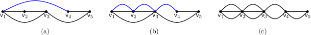
Figure 2.2. Replacing an edge by a path: (a) the original graph with the edge $\mathsf{v}_{1}\mathsf{v}_{4}$ to be replaced shown in blue, (b) the graph obtained after replacing $(\mathsf{v}_{1},\mathsf{v}_{4})$ by three edges with endpoints $(\mathsf{v}_{1},\mathsf{v}_{2})$, $(\mathsf{v}_{2},\mathsf{v}_{3})$ and $(\mathsf{v}_{3},\mathsf{v}_{4})$ respectively (shown in blue), (c) the final graph $\widehat{\mathsf{G}}$ after all replacements prescribed by the proof of Theorem 2.3.

We claim that this operation decreases the Rayleigh quotient of the function $f_{1}$,

$$\mathsf{R}_{p}(\mathsf{G}^{\prime};f_{1})\leq\mathsf{R}_{p}(\mathsf{G};f_{1}).$$

Indeed, this is equivalent to the assertion

(2.6) $$\sum_{\ell=i}^{j-1}|f_{1}(\mathsf{v}_{\ell+1})-f_{1}(\mathsf{v}_{\ell})|^{p}\leq|f_{1}(\mathsf{v}_{j})-f_{1}(\mathsf{v}_{i})|^{p}.$$

Now by using the inequality $\|x\|_{p}\leq\|x\|_{1}$ between the $p$- and $1$-norms of a finite-dimensional vector (which is strict as long as $p>1$ and the vector has more than one nonzero component), applied to

(2.7) $$x:=\big{(}f_{1}(\mathsf{v}_{i+1})-f_{1}(\mathsf{v}_{i}),\ldots,f_{1}(\mathsf{v}_{j})-f_{1}(\mathsf{v}_{j-1})\big{)}\in\mathbb{R}^{j-i},$$

we obtain

$$\left[\sum_{\ell=i}^{j-1}|f_{1}(\mathsf{v}_{\ell+1})-f_{1}(\mathsf{v}_{\ell})|^{p}\right]^{1/p} \leq\sum_{\ell=i}^{j-1}|f_{1}(\mathsf{v}_{\ell+1})-f_{1}(\mathsf{v}_{\ell})|$$

$$=\sum_{\ell=i}^{j-1}f_{1}(\mathsf{v}_{\ell+1})-f_{1}(\mathsf{v}_{\ell})=f_{1}(\mathsf{v}_{j})-f_{1}(\mathsf{v}_{i}),$$

where the first equality here follows from the ordering of the vertices, equation (2.5). Taking the $p$-th power of both sides yields (2.6).

Repeating this operation for every “long edge”, we obtain a pumpkin chain $\widehat{\mathsf{G}}$, which is in general non-regular. Since the graph operation we performed cannot decrease the edge connectivity, $\widehat{\mathsf{G}}$ has edge connectivity at least $\eta$, that is, each pumpkin in $\mathsf{G}_{1}$ has at least $\eta$ parallel edges. We now remove excess edges, producing an $\eta$-regular pumpkin chain $\widetilde{\mathsf{G}}$. It is immediate to see that removing an edge between $v_{i}$ and $v_{i+1}$ also decreases the Rayleigh quotient (strictly decreases if $f_{1}(v_{i})\neq f_{1}(v_{i+1})$).

We therefore have

$$\gamma_{1}^{(p)}(\widetilde{\mathsf{G}})\leq\mathsf{R}_{p}(\widetilde{\mathsf{G}};f_{1})\leq\mathsf{R}_{p}(\widehat{\mathsf{G}};f_{1})\leq\mathsf{R}_{p}(\mathsf{G};f_{1})=\gamma_{1}^{(p)}(\mathsf{G}).$$

This proves the inequality.

To characterize the case of equality we note that it can only happen if the original function $f_{1}$ is also a minimizer of the final graph $\widetilde{\mathsf{G}}$ and thus an eigenfunction. However, it can be shown that any first nontrivial eigenfunction $f_{1}$ of the discrete $p$-Laplacian on a regular pumpkin chain $\widetilde{\mathsf{G}}$ (equivalently, on a path graph) does not take on the same value on neighboring vertices (see e.g. [Spi09, Lemma 2.4.5] for the special case of $p=2$).

For such a test function $f_{1}$, every subdivision of a “long edge” strictly decreases the Rayleigh quotient; so does every removal of an edge. We conclude that no operations can have been performed and therefore $\widetilde{\mathsf{G}}=\mathsf{G}$. ∎

3. Quantum graphs: Estimates based on the edge connectivity

Let us now turn to the case of quantum graphs. It is natural to ask whether we can obtain a result similar to Theorem 1.1 for the smallest nontrivial eigenvalue $\mu_{1}({\mathcal{G}})$ of the Laplacian with natural vertex conditions on the metric graph $\mathcal{G}$, see (1.6). We recall that these vertex conditions require the functions to be continuous at every vertex and the sum of normal derivatives to be zero. But since we are going to work with quadratic forms, it is enough to require that our test functions be continuous at every vertex.

More generally, as in the discrete case, we will in fact consider the smallest nontrivial eigenvalue of the $p$-Laplacian with natural conditions. More precisely, we consider the following weak eigenvalue problem: we call $\mu>0$ an eigenvalue, and $\psi\in W^{1,p}({\mathcal{G}})$ an eigenfunction, if

(3.1) $$\int_{{\mathcal{G}}}|\psi^{\prime}(x)|^{p-2}\psi^{\prime}(x)u^{\prime}(x)\;{\rm d}x=\mu\int_{{\mathcal{G}}}|\psi(x)|^{p-2}\psi(x)u(x)\;{\rm d}x\qquad\text{for all }u\in W^{1,p}({\mathcal{G}}),$$

for fixed $p\in(1,\infty)$. Here the Sobolev space $W^{1,p}({\mathcal{G}})\subset C({\mathcal{G}})$ is defined in the usual way, as the vector space of those edgewise $W^{1,p}$-functions that satisfy continuity conditions in the vertices. The equation (3.1) is the weak form of an eigenvalue problem for the $p$-Laplace operator $-\Delta_{p}$ given by $-\Delta_{p}u=-(|u^{\prime}|^{p-2}u^{\prime})^{\prime}$ on the same metric graph ${\mathcal{G}}$, again with continuity conditions in the vertices along with Kirchhoff-type conditions

(3.2) $$\sum_{\mathsf{e}\sim\mathsf{v}}\left|\frac{\partial}{\partial x}u_{\mathsf{e}}(\mathsf{v})\right|^{p-2}\frac{\partial}{\partial x}u_{\mathsf{e}}(\mathsf{v})=0\qquad\mbox{ for all vertices }\mathsf{v},$$

where the summation is again taken over all edges incident to $\mathsf{v}$ and the derivative is covariant into the edge. (We stress the similarity to (2.3).) If $p=2$, we obviously recover the usual Laplacian. Here and below, we will consider the quantity

(3.3) $$\mu_{1}^{(p)}(\mathcal{G}):=\inf\{\mu>0:\mu\text{ is an eigenvalue in the sense of \eqref{eq:p-lapl-weak-form}}\}.$$

When $p=2$, we recover the smallest nontrivial Laplacian eigenvalue, i.e., $\mu_{1}^{(2)}(\mathcal{G})=\mu_{1}(\mathcal{G})$ defined by (1.6).

We shall also have occasion to consider the first eigenvalue of the $p$-Laplacian with the Dirichlet (zero) condition on a subset $\mathsf{V}_{D}$ of the set of vertices of $\mathcal{G}$. In this case, we shall write $W^{1,p}_{0}(\mathcal{G}):=\{u\in W^{1,p}(\mathcal{G}):u(\mathsf{v})=0\text{ for all }\mathsf{v}\in\mathsf{V}_{D}\}$ and

(3.4) $$\lambda_{1}^{(p)}(\mathcal{G}):=\inf\left\{\frac{\int_{{\mathcal{G}}}|u^{\prime}(x)|^{p}\;{\rm d}x}{\int_{{\mathcal{G}}}|u(x)|^{p}\;{\rm d}x}:u\in W^{1,p}_{0}({\mathcal{G}})\right\}\ ,\qquad p\in(1,\infty)$$

(note that this is now always an eigenvalue, and indeed the very smallest). Of course, both $W^{1,p}_{0}(\mathcal{G})$ and $\lambda_{1}^{(p)}(\mathcal{G})$ depend on the set $\mathsf{V}_{D}$, but in practice it will always be clear which set this is.

We shall keep the following standing assumption on $\mathcal{G}$ throughout the paper, which mirrors Assumption 2.1 for combinatorial graphs.

Assumption 3.1.

The metric graph $\mathcal{G}$ is connected, compact and finite, i.e., it is formed by a finite number $E$ of edges of finite length connected together at a finite number $V$ of vertices. Moreover, we assume that $\mathcal{G}$ does not have any vertices of degree two.

Note that we allow loops (except when we explicitly assume the contrary) and multiple edges.

In order to explain the assumption about vertices of degree two, let us recall that introducing such a vertex for $p=2$, natural vertex conditions imply that both the function and its first derivative are continuous across the vertex. Hence the vertex may be removed and the two edges may be substituted by one longer edge so that the eigenvalues of the quantum graph are preserved as well as its eigenfunctions up to a canonical identification. This is a well-known phenomenon in the theory of quantum graphs when $p=2$. For $p\neq 2$ exactly the same phenomenon can be observed, since any continuous and piecewise-$W^{1,p}$ function belongs to $W^{1,p}$.

We now wish to introduce a notion of edge connectivity for a metric graph $\mathcal{G}$. To cut an edge means to divide it into two smaller edges with the sum of lengths equal to the length of the original edge, keeping the vertices of the original graph and introducing two new degree one vertices. Then it is natural to use the following definition:

Definition 3.2.

Let ${\mathcal{G}}$ be a metric graph. The metric edge connectivity $\eta$ of ${\mathcal{G}}$ is equal to the number of edge cuts needed to make the graph disconnected.

It is clear that the metric edge connectivity is at most two, since one may always cut any given edge twice. In the recent paper [BL16], Band and Lévy obtained the lower bound

(3.5) $$\mu_{1}({\mathcal{G}})=\mu_{1}^{(2)}({\mathcal{G}})\geq\frac{4\pi^{2}}{L^{2}}$$

for all quantum graphs of length $L>0$ and edge connectivity two in this sense. This result includes, in particular, Eulerian graphs, for which the same bound was proved in [KN14, Thm. 2].

The proof of Band and Lévy is based on a refinement of the symmetrization argument introduced by Friedlander [Fri05] used in his proof of the isoperimetric inequality $\mu_{1}({\mathcal{G}})\geq\pi^{2}/L^{2}$. This latter inequality together with (3.5) may be thought of as a natural counterpart to Fiedler’s estimate if we regard the edge connectivity of a quantum graph as being always either one or two.

We shall also introduce discrete edge connectivity, which we believe is better adapted to quantum graphs (despite its name!). In particular, with it we can obtain better bounds if the discrete edge connectivity is more than two.

We have already noticed that degree two vertices can be removed without really affecting the metric graph, leading to equivalent graphs. The only exception is the cycle graph which contains just one vertex, which of course is impossible to eliminate. The discrete edge connectivity will not distinguish between equivalent metric graphs.

Definition 3.3.

Let ${\mathcal{G}}$ be a finite metric graph. If the graph possess vertices of degree two, then consider the equivalent metric graph obtained from ${\mathcal{G}}$ by removing vertices of degree two (if possible). If the number of vertices in the new graph is greater than one, then the discrete edge connectivity $\eta$ of ${\mathcal{G}}$ is the minimal number of edges that need to be deleted in order to make the new graph disconnected.

In the degenerate case of a graph with one vertex (a flower graph including the cycle graph as a special case) we let $\eta=2$.

The discrete edge connectivity is finer; it coincides with the metric one when it is equal to one or two. Henceforth we will use only the discrete connectivity while keeping the same notation $\eta$.

Our main result is as follows.

Theorem 3.4.

Let ${\mathcal{G}}$ be a connected quantum graph of total length $L$ and discrete edge connectivity $\eta$, and let $p\in(1,\infty)$. If $\eta\geq 2$, then

(3.6) $$\mu_{1}^{(p)}(\mathcal{G})\geq(p-1)\left(\frac{2\pi_{p}}{L}\right)^{p}.$$

Moreover, if $\eta\geq 3$, then

(3.7) $$\mu_{1}^{(p)}({\mathcal{G}})\geq(p-1)\left(\frac{\eta\pi_{p}}{L+\ell_{\max}(\eta-2)}\right)^{p},$$

where $\ell_{\max}$ is the length of the longest edge of $\mathcal{G}$.

Here

$$\pi_{p}:=\frac{2\pi}{p\sin\frac{\pi}{p}}\ .$$

It is known that $\pi_{p}$ is the smallest positive root of $\sin_{p}$, defined on $[0,\frac{\pi_{p}}{2}]$ as the inverse of

$$s\mapsto\int_{0}^{x}(1-s^{p})^{-\frac{1}{p}}\ ds$$

and then suitably extended to $\mathbb{R}$ by reflection and periodicity. The values on the right hand sides of (3.6) and (3.7) correspond to the first nontrivial eigenvalue of the Neumann Laplacian on an edge of length $L/2$ and $(L+\ell_{\max}(\eta-2))/\eta$, respectively. See, e.g., the monograph [LE11] for more details.

Corollary 3.5.

Under the assumptions of Theorem 3.4 we have in particular for $p=2$

(3.8) $$\mu_{1}(\mathcal{G})\geq\frac{\eta^{2}\pi^{2}}{(L+\ell_{\max}(\eta-2)_{+})^{2}}.$$

Remark 3.6.

(a) The estimate (3.6) is sharp, but (3.7) is not, except asymptotically for certain sequences of graphs for which $\ell_{\max}\to 0$, provided $\eta$ is kept fixed. To give examples, we will need details from the proof of Theorem 3.4 (including classes of graphs which will be introduced there). Hence we defer the proof of both statements until after this proof; see Remark 3.8. There, we also characterize the case of equality in (3.6). This was already treated in [BL16] when $p=2$.

(b) A correction term along the lines of $(\eta-2)\ell_{\max}$ is however necessary if $\eta\geq 3$. It may be viewed as consequence of using the discrete edge connectivity. Indeed, a lower bound of the form $\pi_{p}^{p}\eta^{p}/L^{p}$ is obviously impossible, even for $p=2$: take, for example, a very small pumpkin on $\eta$ slices and attach a single, very long loop to one of its vertices.

(c) The bound in (3.7) is an increasing function of $\eta\geq 2$ if (and only if) $L\geq 2\ell_{\max}$. This follows from the fact that the length of the comparison interval, i.e., $(L+(\eta-2)_{+}\ell_{\max})/\eta$, is a decreasing function of $\eta\geq 2$ if and only if $L\geq 2\ell_{\max}$, together with the fact that the first eigenvalue of an interval is a decreasing function of the latter’s length, for any $p\in(1,\infty)$. An inspection of the proof of Theorem 3.4 shows that in fact

$$\mu_{1}^{(p)}(\mathcal{G})\geq(p-1)\left(\frac{h\pi_{p}}{L+(h-2)\ell_{\max}}\right)^{p}$$

for all $1\leq h\leq\eta$ (just replace $\eta$ with $h$ throughout). Hence we may obtain a better bound than (3.7) by taking the maximum over such $h$ if $L<2\ell_{\max}$. Moreover, in the case $L<2\ell_{\max}$, i.e., if a single edge “dominates” $\mathcal{G}$, then, by taking as a test function an appropriate $p$-sinusoidal curve on the longest edge extended by zero elsewhere on $\mathcal{G}$, we can obtain a trivial upper bound which shows $\mu_{1}^{(p)}$ is essentially proportional to the longest edge length, meaning algebraic quantities such as edge connectivity are less relevant. For example, if $p=2$, this test function argument yields

$$\mu_{1}({\mathcal{G}})\leq\frac{4\pi^{2}}{(\ell_{\max})^{2}}$$

to complement the lower bound of (3.5), namely

$$\mu_{1}({\mathcal{G}})\geq\frac{4\pi^{2}}{L^{2}}\geq\frac{\pi^{2}}{(\ell_{\max})^{2}}.$$

Let us now prepare for the proof of Theorem 3.4. We will need the following simple lemma, which provides an important technical link between the edge connectivity (in both discrete and continuous form) and the behavior of any $p$-Laplacian eigenfunction.

We will first need the following notation: denoting by $\mu>0$ any given eigenvalue of (3.1) and by $\psi\in W^{1,p}({\mathcal{G}})\subset C({\mathcal{G}})$ any eigenfunction corresponding to $\mu$, we set

(3.9) $$\begin{split}\mathcal{G}_{+}&:=\{x\in{\mathcal{G}}:\psi(x)>0\},\\ \mathcal{G}_{-}&:=\{x\in{\mathcal{G}}:\psi(x)<0\},\\ \operatorname{\mathcal{G}}(t)&:=\{x\in{\mathcal{G}}:\psi(x)=t\},\qquad t\in\mathbb{R},\end{split}$$

noting that since $\mu>0$, both $\mathcal{G}_{+}$ and $\mathcal{G}_{-}$ must be nonempty. (Just take $u(x)=1$ in (3.1) to obtain the “$p$-orthogonality condition” $\int_{{\mathcal{G}}}|\psi(x)|^{p-2}\psi(x)\;{\rm d}x=0$, which forces $\psi$ to change sign in ${\mathcal{G}}$.) In general, $\mathcal{G}_{\pm}$ will not be connected. We also denote by

$$\nu(t):=\#\operatorname{\mathcal{G}}(t)$$

the size of the level “surface” of $\psi$ at $t$, noting this is finite whenever $t\neq 0$ as our graph is finite; it is possible that $\psi$ is identically zero on some edge of ${\mathcal{G}}$, in which case we write $\nu(0)=\infty$; observe that $0$ is the only constant value that can be attained by an eigenfunction of a nonzero eigenvalue on an open interval in ${\mathcal{G}}$. Finally, we denote by

$$\mathfrak{S}:=\psi(\mathsf{V})\equiv\{\psi(\mathsf{v}):\mathsf{v}\in\mathsf{V}\}$$

the (finite) set of all values $\psi$ attains at the vertex set of ${\mathcal{G}}$ and by

$$\mathfrak{S}^{\ast}:=\mathfrak{S}\cup\{\max_{x\in{\mathcal{G}}}\psi(x),\min_{x\in{\mathcal{G}}}\psi(x)\}$$

the complete (and still finite) set of “exceptional values” of $\psi$.

Lemma 3.7.

Suppose with the above notation that the discrete edge connectivity $\eta\geq 2$. Then

1. $\nu(t)\geq 2$ for all $t\in(\min_{x\in{\mathcal{G}}}\psi(x),\max_{x\in{\mathcal{G}}}\psi(x))\setminus\mathfrak{S}$;

2. $\nu(t)\geq\eta$ for all $t\in(\min\mathfrak{S},\max\mathfrak{S})\setminus\mathfrak{S}$.

Proof.

(i) If $t\in(\min_{x\in{\mathcal{G}}}\psi(x),\max_{x\in{\mathcal{G}}}\psi(x))$, then the graph ${\mathcal{G}}\setminus\operatorname{\mathcal{G}}(t)$ must be disconnected, as it cannot contain any further path from the location of the minimum of $\psi$ to the location of the maximum. That is, removing $\operatorname{\mathcal{G}}(t)$ cuts the graph into (at least) two pieces. Since $t\not\in\mathfrak{S}$, we have $\operatorname{\mathcal{G}}(t)\cap\mathsf{V}=\emptyset$. Our assumption on connectivity implies $\nu(t)=\#\operatorname{\mathcal{G}}(t)\geq 2$.

(ii) Similarly, for $t\in(\min\mathfrak{S},\max\mathfrak{S})$, the graph ${\mathcal{G}}\setminus\operatorname{\mathcal{G}}(t)$ is disconnected, since there is no path left connecting the vertices of ${\mathcal{G}}$ at which $\min\mathfrak{S}$ and $\max\mathfrak{S}$ are attained. Since $t\not\in\mathfrak{S}$, the set of edges containing $\operatorname{\mathcal{G}}(t)$ must have cardinality at least $\eta$, since its removal leads to a disconnected (discrete) graph. ∎

We emphasize that the restriction in (ii) to those values of $\psi$ between its minimal and maximal vertex values is essential, as is easy to see in the following example: if $\psi$ has a unique maximum achieved in the interior of an edge, then for $t$ close to this value we will have $\nu(t)=2$ regardless of the discrete edge connectivity.

Proof of Theorem 3.4.

The proof is based on a sharper version of the symmetrization procedure of Friedlander [Fri05, Lemma 3], which was introduced on Eulerian graphs in the work of Kurasov and Naboko [KN14] and on graphs where $\eta=2$ in the work of Band and Levy [BL16]. Here we sharpen this approach further for higher values of $\eta$.

We start by fixing an arbitrary eigenvalue $\mu>0$ and any eigenfunction $\psi$ associated with it; this also fixes the corresponding sets $\mathcal{G}_{+}$, $\mathcal{G}_{-}$, as well as the function $\nu(t)$ and so forth. Obviously, it suffices to prove the theorem for this $\mu>0$.

We first observe that we may assume without loss of generality that

(3.10) $$\max\mathfrak{S}=\operatorname{ess\,sup}\{t\in\mathbb{R}:\nu(t)\geq\eta\},$$

and that this maximum is attained at a single vertex, call it $\mathsf{v}_{\max}$. Indeed, Lemma 3.7(ii) yields “$\leq$”, and if we have strict inequality, then we may insert artificial vertices at all points $x\in\mathcal{G}$ where $\psi(x)$ is equal to this supremum and form a new graph, call it ${\mathcal{G}}^{\prime}$, by identifying them. Then ${\mathcal{G}}^{\prime}$ still has edge connectivity $\geq\eta$ by construction. Moreover, $\psi$ may be canonically identified with a function in $W^{1,p}({\mathcal{G}}^{\prime})$; moreover, since $W^{1,p}({\mathcal{G}}^{\prime})$ may be canonically identified with a subset of $W^{1,p}({\mathcal{G}})$, it follows that (3.1) continues to hold on ${\mathcal{G}}^{\prime}$. Hence $(\mu,\psi)$ is, up to this identification, also an eigenpair of ${\mathcal{G}}^{\prime}$ and we may consider it instead. To keep notation simple, we will write ${\mathcal{G}}$ in place of ${\mathcal{G}}^{\prime}$.

If $\eta=2$, then $\psi$ attains its maximum over $\mathcal{G}$ at $\mathsf{v}_{\max}$; if $\eta\geq 3$, this is not guaranteed.

We may also assume without loss of generality that $|\mathcal{G}_{+}|\leq L/2$ (where $|\,\cdot\,|$ denotes Lebesgue measure, i.e., length). We will denote by $W^{1,p}_{0}(\mathcal{G}_{+})$ those $W^{1,p}(\mathcal{G}_{+})$-functions which are zero on the boundary of $\mathcal{G}_{+}$ in $\mathcal{G}$, which by standard properties of Sobolev functions may be characterized by

$$W^{1,p}_{0}(\mathcal{G}_{+})=\{u\in W^{1,p}(\mathcal{G}_{+}):\text{ there exists }\tilde{u}\in W^{1,p}(\mathcal{G})\text{ with }\tilde{u}\equiv 0\text{ on }\mathcal{G}\setminus\mathcal{G}_{+},\,u=\tilde{u}|_{\mathcal{G}_{+}}\}.$$

In particular, $\psi\equiv\psi|_{\mathcal{G}_{+}}\in W^{1,p}_{0}(\mathcal{G}_{+})$. Moreover,

$$\mu=\frac{\int_{\mathcal{G}_{+}}|\psi^{\prime}|^{p}\,dx}{\int_{\mathcal{G}_{+}}|\psi|^{p}\,dx}\ ,$$

as can be seen by taking $\psi_{+}:=\psi\cdot\chi_{\mathcal{G}_{+}}\in W^{1,p}(\mathcal{G})$ as a test function in (3.1).

We now associate with $\mathcal{G}_{+}$ a “symmetrized” half pumpkin with loops attached to one end – a stower, in the terminology of the recent paper [BL16]. More precisely, we start by considering the set which we shall wish to symmetrize,

$$\mathcal{G}_{\mathfrak{S}}:=\{x\in\mathcal{G}_{+}:\psi(x)\leq\max\mathfrak{S}\}.$$

By definition of, and our assumptions on, $\mathfrak{S}$, the open set $\mathcal{G}_{+}\setminus\mathcal{G}_{\mathfrak{S}}$ has no vertices and thus consists of some number $n\geq 0$ of individual edges, each having both endpoints at $\mathsf{v}_{\max}$, say $e_{1},\ldots,e_{n}$, which represent the set where $\psi>\max\mathfrak{S}$. By (3.10), $2n<\eta$; in particular, $n=0$ if $\eta=2$.

We now form a new graph $\mathcal{G}_{+}^{\ast}$ by attaching $\eta$ equal edges $\tilde{e}_{1},\ldots,\tilde{e}_{\eta}$ of length $|\mathcal{G}_{\mathfrak{S}}|/\eta$ to each other at a common vertex $\mathsf{v}_{0}$ (i.e. to form a star; for each $i$, we denote the other vertex of edge $\tilde{e}_{i}$ by $\tilde{\mathsf{v}}_{i}$). We identify each edge $\tilde{e}_{i}$ with the interval $[0,|\mathcal{G}_{\mathfrak{S}}|/\eta]$, whose right hand endpoint corresponds to the central vertex $\mathsf{v}_{0}$. To $\mathsf{v}_{0}$ we also attach $n$ loops $\hat{e}_{1},\ldots,\hat{e}_{n}$ emanating from $\mathsf{v}_{0}$, having lengths $|e_{1}|,\ldots,|e_{n}|$, respectively, see Fig. 3.1(a).

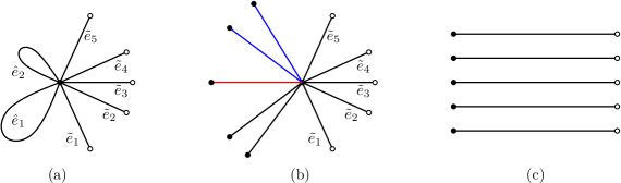
Figure 3.1. The symmetrized graph $\mathcal{G}_{+}^{\ast}$ and its modifications. Black and white dots represent vertices with Neumann and Dirichlet boundary conditions, respectively. (b) shows the graph $\widehat{\mathcal{G}}_{+}$, which has been formed from (a) by lengthening $\hat{e}_{2}$ (edges in blue), splitting the loops apart, and adding an edge (red) so that there are as many edges with a Neumann endpoint as Dirichlet ones.

We now construct, for each $\phi\in W^{1,p}_{0}(\mathcal{G}_{+})$, a “symmetrized” function $\phi^{\ast}$ on $\mathcal{G}_{+}^{\ast}$ as follows: on each of the edges $\tilde{e}_{i}\simeq[0,|\mathcal{G}_{\mathfrak{S}}|/\eta]$ we set $\phi^{\ast}(0)=0$ and

(3.11) $$|\{x\in(0,|\mathcal{G}_{\mathfrak{S}}|/\eta):\phi^{\ast}(x)<t\}|=\frac{1}{\eta}\,|\{x\in\mathcal{G}_{\mathfrak{S}}:\phi(x)<t\}|$$

for all $t\in\mathbb{R}$. We then set $\phi^{\ast}(\mathsf{v}_{0}):=\phi(\mathsf{v}_{\max})$ and extend $\phi^{\ast}$ to the loops $\hat{e}_{i}$ in the obvious way, by mapping the values of $\phi$ on each loop $e_{i}$ onto the corresponding $\hat{e}_{i}$, $i=1,\ldots,n$. By standard results on symmetrization, the resulting function $\phi^{\ast}$ is continuous across $\mathcal{G}_{+}^{\ast}$ and in $W^{1,p}$ on each edge, so we conclude $\phi^{\ast}\in W^{1,p}(\mathcal{G}_{+}^{\ast})$.

Moreover, by construction and Cavalieri’s principle,

$$\|\phi^{\ast}\|_{L^{p}(\mathcal{G}_{+}^{\ast})}=\|\phi\|_{L^{p}(\mathcal{G}_{+})}\ ,$$

and

$$\sum_{x\in\mathcal{G}(t)}\frac{1}{|\psi^{\prime}(x)|}=\frac{\eta}{|(\psi^{\ast})^{\prime}(y_{t})|}$$

for almost all $t\in(0,\max\mathfrak{S})$, where $y_{t}$ is any point in $\bigcup_{i=1}^{\eta}\tilde{e}_{i}$ such that $\psi^{\ast}(y_{t})=t$.

Obviously,

$$\|(\phi^{\ast})^{\prime}\|_{L^{p}\left(\bigcup_{i=1}^{n}\hat{e}_{i}\right)}=\|\phi^{\prime}\|_{L^{p}\left(\bigcup_{i=1}^{n}e_{i}\right)}.$$

We will now show for the eigenfunction $\psi$ and its symmetrization $\psi^{\ast}$ that

(3.12) $$\|(\psi^{\ast})^{\prime}\|_{L^{p}\left(\bigcup_{i=1}^{\eta}\tilde{e}_{i}\right)}\leq\|\psi^{\prime}\|_{L^{p}(\mathcal{G}_{\mathfrak{S}})}.$$

(In fact, (3.12) holds with the same argument for any $\phi\in W^{1,p}_{0}(\mathcal{G}_{+})$, but this keeps the notation simpler and certain technical issues involving regularity do not arise.) To see this, we use ideas similar to [Fri05, Lemma 3] but make use of Lemma 3.7. By the coarea formula,

$$\int_{\mathcal{G}_{\mathfrak{S}}}|\psi^{\prime}|^{p}\,dx=\int_{0}^{\max\mathfrak{S}}\sum_{x\in\mathcal{G}(t)}|\psi^{\prime}(x)|^{p-1}\,dt.$$

By Hölder’s inequality and Lemma 3.7(ii), for almost all $t\in(0,\max\mathfrak{S})$, we have

$$\nu(t)=\sum_{x\in\mathcal{G}(t)}1=\sum_{x\in\mathcal{G}(t)}|\psi^{\prime}(x)|^{\frac{p-1}{p}}\cdot\left(\frac{1}{|\psi^{\prime}(x)|}\right)^{\frac{p-1}{p}}\leq\left(\sum_{x\in\mathcal{G}(t)}|\psi^{\prime}(x)|^{p-1}\right)^{\frac{1}{p}}\left(\sum_{x\in\mathcal{G}(t)}\frac{1}{|\psi^{\prime}(x)|}\right)^{\frac{p-1}{p}},$$

noting that $\psi^{\prime}\neq 0$ almost everywhere on $\mathcal{G}_{+}$. Rearranging,

$$\sum_{x\in\mathcal{G}(t)}|\psi^{\prime}(x)|^{p-1}\geq\nu(t)^{p}\left(\sum_{x\in\mathcal{G}(t)}\frac{1}{|\psi^{\prime}(x)|}\right)^{-(p-1)}\geq\eta^{p}\left(\sum_{x\in\mathcal{G}(t)}\frac{1}{|\psi^{\prime}(x)|}\right)^{-(p-1)}.$$

Hence

$$\begin{split}\int_{\mathcal{G}_{\mathfrak{S}}}|\psi^{\prime}|^{p}\,dx&=\int_{0}^{\max\mathfrak{S}}\sum_{x\in\mathcal{G}(t)}|\psi^{\prime}(x)|^{p-1}\,dt\geq\eta^{p}\int_{0}^{\max\mathfrak{S}}\left(\sum_{x\in\mathcal{G}(t)}\frac{1}{|\psi^{\prime}(x)|}\right)^{-(p-1)}\,dt\\ &=\eta^{p}\int_{0}^{\max\mathfrak{S}}\left(\frac{\eta}{|(\psi^{\ast})^{\prime}(y_{t})|}\right)^{-(p-1)}\,dt=\eta\int_{0}^{\max\mathfrak{S}}|(\psi^{\ast})^{\prime}(y_{t})|^{p-1}\,dt.\end{split}$$

Another application of the coarea formula yields

$$\eta\int_{0}^{\max\mathfrak{S}}|(\psi^{\ast})^{\prime}(y_{t})|^{p-1}\,dt=\int_{\bigcup_{i=1}^{\eta}\tilde{e}_{i}}|(\psi^{\ast})^{\prime}(x)|^{p}\,dx,$$

recalling that $\psi^{\ast}$ is equal on each edge $\tilde{e}_{i}$. This completes the proof of (3.12). We have now shown that

$$\mu=\frac{\int_{\mathcal{G}_{+}}|\psi^{\prime}|^{p}\,dx}{\int_{\mathcal{G}_{+}}|\psi|^{p}\,dx}\geq\frac{\int_{\mathcal{G}_{+}^{\ast}}|(\psi^{\ast})^{\prime}|^{p}\,dx}{\int_{\mathcal{G}_{+}^{\ast}}|\psi^{\ast}|^{p}\,dx}\geq\lambda_{1}^{(p)}(\mathcal{G}_{+}^{\ast}),$$

where $\lambda_{1}^{(p)}(\mathcal{G}_{+}^{\ast})$ is the first $p$-Laplacian eigenvalue of $\mathcal{G}_{+}^{\ast}$ with the natural condition at the central vertex $\mathsf{v}_{0}$ and Dirichlet conditions at the other vertices $\tilde{\mathsf{v}}_{1},\ldots,\tilde{\mathsf{v}}_{\eta}$ (cf. (3.4)).

If $\eta=2$, then $\mathsf{v}_{0}$ has degree two and $\lambda_{1}^{(p)}(\mathcal{G}_{+}^{\ast})$ is the first eigenvalue of the Dirichlet $p$-Laplacian on an interval of length $2\cdot|\mathcal{G}_{\mathfrak{S}}|/\eta=|\mathcal{G}_{\mathfrak{S}}|=|\mathcal{G}_{+}|\leq L/2$, which is obviously in turn no smaller than the smallest nontrivial $p$-Laplacian eigenvalue of a loop of length $L$, or equivalently, of an interval of length

$$\frac{L}{2}=\frac{L+\ell_{\max}(\eta-2)}{\eta},\qquad\eta=2,$$

with Neumann conditions at its endpoints. Since the lowest nonzero eigenvalue of the $p$-Laplacian with Neumann boundary conditions on an interval of length $\ell$ is in fact

$$(p-1)\left(\frac{\pi_{p}}{\ell}\right)^{p}$$

(see, e.g., [LE11, Thm. 3.4]), this proves (3.6).

If $\eta\geq 3$, we need to account for the possibility of loops $\hat{e}_{1},\ldots,\hat{e}_{n}$, $n\geq 0$, at $\mathsf{v}_{0}$. To this end, we first suppose that $\hat{e}_{1}$ is the longest loop at $\mathsf{v}_{0}$ and lengthen the others if necessary to make them all exactly as long. We next “split apart” each loop in its midpoint, i.e., we create a new graph with no loops but $2n$ pendant edges at $\mathsf{v}_{0}$ of equal length $|\hat{e}_{1}|/2$, all having the Neumann condition at their free endpoint. Recalling that $2n<\eta$, we next attach $\eta-2n$ additional pendant edges of length $|\hat{e}_{1}|/2$ to $\mathsf{v}_{0}$, again with Neumann conditions at the free ends. Easy variational arguments similar to the ones in [BK13, Thm 3.1.10] or [KKMM16, Lemma 2.3] show that every step of this process can only decrease $\lambda_{1}^{(p)}(\mathcal{G}_{+}^{\ast})$.

We claim that the resulting graph, call it $\widehat{\mathcal{G}}_{+}$, see Fig. 3.1(b), has first eigenvalue $\lambda_{1}^{(p)}(\widehat{\mathcal{G}}_{+})$ no smaller than the smallest nontrivial Neumann $p$-Laplace eigenvalue of an interval of length

$$\frac{L+(\eta-2)|\hat{e}_{1}|}{\eta}.$$

Since there must have been an edge in the original graph $\mathcal{G}$ at least as long as $\hat{e}_{1}$, we have $|\hat{e}_{1}|\leq\ell_{\max}$. Since $\mu_{1}^{(p)}$ on an interval is a decreasing function of the interval’s length and since we have shown $\mu_{1}^{(p)}(\mathcal{G})\geq\lambda_{1}^{(p)}(\mathcal{G}_{+})$, this claim will complete the proof of the theorem.

To prove the claim, we observe that $\widehat{\mathcal{G}}_{+}$ consists of $\eta$ identical copies of an interval of length $|\hat{e}_{1}|/2+\mathcal{G}_{\mathfrak{S}}/\eta$, where the vertex conditions corresponding to $\lambda_{1}^{(p)}(\mathcal{G}_{+})$ consist of a Neumann condition at one end and a Dirichlet one at the other of each interval; all these copies are joined together at the common vertex $\mathsf{v}_{0}$ at a distance $|\hat{e}_{1}|/2$ from the Neumann end, as in Fig. 3.1(b). The obvious bijection between (nonnegative) eigenfunctions on the two graphs shows that the first eigenvalue of $\widehat{G}_{+}$ is equal to the first eigenvalue of any of these intervals, which each have length

$$\frac{|\hat{e}_{1}|}{2}+\frac{|\mathcal{G}_{\mathfrak{S}}|}{\eta}\leq\frac{|\hat{e}_{1}|}{2}+\left(\frac{L}{2}-|\hat{e}_{1}|\right)\frac{1}{\eta}=\frac{L+(\eta-2)|\hat{e}_{1}|}{2\eta},$$

since $|\mathcal{G}_{\mathfrak{S}}|\leq|\mathcal{G}_{+}|-|\hat{e}_{1}|$ and $|\mathcal{G}_{+}|\leq L/2$ by assumption. But the first eigenvalue of the $p$-Laplacian on an interval of length $(L+(\eta-2)\ell_{\max})/(2\eta)$ with a Dirichlet condition at one end and a Neumann one at the other is equal to the smallest nontrivial Neumann eigenvalue of an interval of twice the length, $(L+(\eta-2)\ell_{\max})/\eta$. This proves the claim. ∎

Remark 3.8 (The case of equality).

(a) Equality in (3.6) holds if and only if $\mathcal{G}$ is a finite chain of cycles – more precisely, in the terminology of Section 2, a $2$-pumpkin chain, where the two edges in each pumpkin are as long as each other, and where each of the two terminal vertices may have a loop attached to it. In [BL16], these are called symmetric necklace graphs and identified as the corresponding minimizers when $p=2$; they are exactly those graphs having the same first nontrivial eigenvalue as a loop, among all graphs of edge connectivity at least two with a given total length. (In particular, one may show that $\mu_{1}^{(p)}$ is in fact an eigenvalue on such graphs.)

To see this, first observe that equality implies $|\mathcal{G}_{+}|=L/2$. Then also $|\mathcal{G}_{-}|=L/2$, because if the eigenfunction were to vanish on a set of positive length, we could make $\mathcal{G}$ strictly smaller without changing the eigenvalue. Moreover, since

$$\frac{\int_{\mathcal{G}_{+}}|\psi^{\prime}|^{p}\,dx}{\int_{\mathcal{G}_{+}}|\psi|^{p}\,dx}=\frac{\int_{\mathcal{G}_{+}^{\ast}}|(\psi^{\ast})^{\prime}|^{p}\,dx}{\int_{\mathcal{G}_{+}^{\ast}}|\psi^{\ast}|^{p}\,dx},$$

we must have $\nu(t)=\eta=2$ for almost all $t\in[0,\max\psi]$. Thus up to a finite exceptional set, $\mathcal{G}$ must consist of two paths representing the preimages of the set $(\min\psi,\max\psi)$. This is only possible if $\mathcal{G}$ is a cycle or a pumpkin chain of degree two (with loops at each end under the convention that no vertex may have degree two). That the pumpkin chain must be regular can be shown by noting that to have equality in Hölder’s inequality, we need $|\psi^{\prime}(x)|=|\psi^{\prime}(y)|$ for any $x$ and $y$ in the same $\operatorname{\mathcal{G}}(t)$. Therefore, the function $\psi$ is identical along the two paths, and, in particular, the paths have the same length.

(b) Equality in (3.7) never holds. This follows since we always have $\lambda_{1}^{(p)}(\mathcal{G}_{+}^{\ast})>\lambda_{1}^{(p)}(\widehat{\mathcal{G}}_{+})$ if $\eta\geq 3$: equality would require $\mathcal{G}_{+}^{\ast}$ to have exactly $\eta/2$ loops of length $|\hat{e}_{1}|$ at $\mathsf{v}_{0}$, but we already observed that $n<\eta/2$. However, equality for fixed $\eta\geq 3$ and $L>0$ is attained in the asymptotic limit for some classes of graphs as $\ell_{\max}\to 0$ (and hence the number of edges tends to infinity). To show this, it is enough to construct a sequence of graphs with constant $\mu_{1}^{(p)}(\mathcal{G}_{n})$ but $\ell_{\max}(\mathcal{G}_{n})\to 0$. This is achieved, for example, by $\eta$-regular pumpkin chains with $n$ pumpkins and edges of equal length (which works out to be $L/n\eta$).

(c) If we happen to know that $\mu_{1}^{(p)}(\mathcal{G})$ has an eigenfunction which attains its maximum and minimum on vertices of $\mathcal{G}$, then the proof of Theorem 3.4 in fact yields

$$\mu_{1}^{(p)}(\mathcal{G})\geq\left(\frac{\eta\pi_{p}}{L}\right)^{p}\ ;$$

in particular, $\mu_{1}(\mathcal{G})\geq\pi^{2}\eta^{2}/L^{2}$. This follows because in this case $\mathcal{G}_{+}^{\ast}$ does not have any loops.

Remark 3.9.

As mentioned in the introduction, Fiedler derived both a lower and an upper estimate on the spectral gap of the discrete Laplacian on combinatorial graphs based on the edge connectivity $\eta$. We are not aware of upper estimates on the spectral gap of the differential Laplacian on quantum graphs based on $\eta$, and indeed this does not appear to be a natural quantity for upper bounds. Indeed, a small perturbation of a graph with large $\eta$ can greatly decrease $\eta$ without significantly affecting the eigenvalues. Consider, for example, a sequence of “pumpkin dumbbells” ${\mathcal{G}}_{n}$ – each consisting of two identical pumpkins, both having $k_{n}$ edges, joined by a single, short edge (a “handle”). Then we can let $k_{n}\to\infty$ while keeping the total length fixed $L>0$, by shrinking the edges correspondingly. If the handle also shrinks, then we can expect $\mu_{1}^{(p)}({\mathcal{G}}_{n})\to\infty$ (for $p=2$ this follows from [KKMM16, Thm. 7.2], since the diameter of ${\mathcal{G}}_{n}$ tends to zero). Thus it is possible that $\eta$ and $L$ remain fixed, while $\mu_{1}^{(p)}\to\infty$. One could ask whether we might obtain a bound if we impose a minimum on $\ell_{\min}$, but we leave open the question of whether it is then possible to do better than trivial bounds in terms of $\ell_{\min}$ alone such as

$$(p-1)\left(\frac{2\pi_{p}}{\ell_{\min}}\right)^{p},$$

corresponding to the first eigenvalue of the Dirichlet $p$-Laplacian on an interval of length $\ell_{\min}/2$.

3.1. Implications for the normalized Laplacian

Let us mention a tangential but notable consequence of Theorem 3.4: von Below [Bel85] observed a transference principle for the spectra of the differential Laplacian on an equilateral metric graph ${\mathcal{G}}$ and of the normalized Laplacian $\mathcal{L}_{\rm norm}$ on the underlying combinatorial graph $\mathsf{G}$, cf. [Chu97]. If all edges of ${\mathcal{G}}$ have the same length (without loss of generality, length 1), then the spectral gap $\mu_{1}({\mathcal{G}})=\mu_{1}^{(2)}({\mathcal{G}})$ of the differential Laplacian and the lowest nonzero eigenvalue

$$\alpha_{1}(\mathsf{G}):=\inf\left\{\frac{\sum\limits_{\mathsf{e}\in\mathsf{E}}|f(\mathsf{e}_{init})-f(\mathsf{e}_{term})|^{2}}{\sum\limits_{\mathsf{v}\in\mathsf{V}}|f(\mathsf{v})|^{2}\deg(\mathsf{v})}:\,0\neq f\in\mathbb{R}^{\mathsf{V}},\,\sum_{\mathsf{v}\in\mathsf{V}}f(\mathsf{v})\deg(\mathsf{v})=0\right\}\in[0,2]$$

of the normalized Laplacian $\mathcal{L}_{\rm norm}$ satisfy the equality

(3.13) $$\mu_{1}({\mathcal{G}})=\left(\arccos(1-\alpha_{1}(\mathsf{G}))\right)^{2},$$

provided $\alpha_{1}(\mathsf{G})\in[0,2)$ (the restriction $\alpha_{1}(\mathsf{G})\neq 2$ may actually be dropped unless $\mathsf{G}$ is a non-bipartite unicyclic graph, in which case $\pi^{2}$ will be an eigenvalue of the differential Laplacian even if $2$ is not an eigenvalue of $\mathcal{L}_{\rm norm}$). By definition, $\alpha_{1}(\mathsf{G})$ is related to the lowest nonzero eigenvalue $\gamma_{1}(\mathsf{G})$ of $\mathcal{L}$ by

(3.14) $$\alpha_{1}(\mathsf{G})\deg_{\rm max}(\mathsf{G})\geq\gamma_{1}(\mathsf{G})\geq\alpha_{1}(\mathsf{G})\deg_{\rm min}(\mathsf{G})\ ,$$

where $\deg_{\min}(\mathsf{G})$ and $\deg_{\max}(\mathsf{G})$ are the minimal and maximal degree of the graph, respectively. Thus, combining (3.14) and (1.1) we obtain the lower estimate

(3.15) $$\alpha_{1}(\mathsf{G})\geq\frac{2\eta}{\deg_{\max}(\mathsf{G})}\left[1-\cos\left(\frac{\pi}{V}\right)\right]\ ;$$

as an essentially trivial consequence of (3.7); but apart from this, no further estimate on $\alpha_{1}$ based on $\eta$ seems to have appeared in the literature so far and in fact the spectral properties of these two matrices are known to be rather different – the normalized Laplacian mirroring the geometry of a combinatorial graph in a more reliable way.

Combining Corollary 3.5 with (3.13) we obtain

Corollary 3.10.

Let $\mathsf{G}$ be a combinatorial graph on $E$ edges with edge connectivity $\eta$. Then the lowest nonzero eigenvalue $\alpha_{1}(\mathsf{G})$ of the normalized Laplacian $\mathcal{L}_{\rm norm}$ satisfies

(3.16) $$\alpha_{1}(\mathsf{G})\geq 1-\cos\left(\frac{\pi\eta}{E+(\eta-2)_{+}}\right).$$

To the best of our knowledge this is also the first instance of estimates of combinatorial spectral graph theory obtained by quantum graph methods, instead of the other way around. It is not known whether von Below’s formula (3.13) also extends to the case of $p$-Laplacians for $p\neq 2$ and we thus do not know whether (3.16) can also be extended to the case of normalized $p$-Laplacians on combinatorial graphs.

Example 3.11.

Using $\cos x\simeq 1-x^{2}/2$ one obtains the asymptotic behavior

$$\frac{2\eta}{\deg_{\max}(\mathsf{G})}\frac{\pi^{2}}{2V^{2}}\qquad\hbox{and}\qquad\frac{\pi^{2}\eta^{2}}{2(E+(\eta-2)_{+})^{2}}$$

as $V,E\to\infty$, respectively, for the right hand sides of (3.14) and (3.16). Let us consider the case of a wheel graph $\mathsf{W}_{n+1}$ on $n+1$ vertices, which has $2n$ edges, whose maximal degree is $n$ and whose discrete edge connectivity is 3. Then the lower estimates become

$$\frac{3\pi^{2}}{n^{3}}\qquad\hbox{and}\qquad\frac{9\pi^{2}}{2(2n+1)^{2}}$$

which shows that our estimate is substantially better. The correct spectral gap of the wheel graph was computed in [But08, § 2.3.1] to be

$$\alpha_{1}(\mathsf{W}_{n+1})=1-\frac{2}{3}\cos\frac{2\pi}{n},$$

to be compared with our estimate

$$\alpha_{1}(\mathsf{W}_{n+1})\geq 1-\cos\frac{3\pi}{2n+1}\ .$$

4. Eigenvalue estimates for graphs with Dirichlet vertices

Our main tools in this section will be a symmetrization argument similar to the one in the proof of Theorem 3.4 and the following Lemma established by Band, Berkolaiko and Weyand.

Lemma 4.1 (Lemma 4.2 of [BBW15]).

Let ${\mathcal{G}}$ be a metric graph with a vertex $v$ of degree $d$ with natural conditions, whose removal separates the graph into $d$ disjoint subgraphs. We denote its edge set by $E_{v}$. Let $r<d$ be a nonnegative integer. For a subset $E_{D}$ of $E_{v}$, with $\left|E_{D}\right|=r$, define ${\mathcal{G}}_{E_{D}}$ to be the modification of the graph ${\mathcal{G}}$ obtained by imposing the Dirichlet condition at $v$ for edges from $E_{D}$ and leaving the edges from $E_{v}\setminus E_{D}$ connected at $v$ with the natural condition (see Figure 4.1 for an example). Then

(4.1) $$\lambda_{n-1}({\mathcal{G}})\leq\min_{|E_{D}|=r}\lambda_{n}({\mathcal{G}}_{E_{D}})\leq\lambda_{n}({\mathcal{G}})\leq\max_{|E_{D}|=r}\lambda_{n}({\mathcal{G}}_{E_{D}})\leq\lambda_{n+1}({\mathcal{G}}).$$

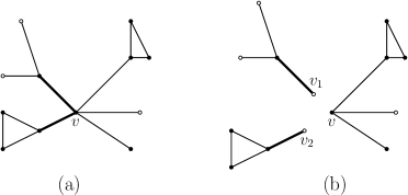
Figure 4.1. A graph ${\mathcal{G}}$ and one possibility of its modification ${\mathcal{G}}_{E_{D}}$ as in Lemma 4.1 with $r=2$. Dirichlet vertices are shown as empty circles.

Remark 4.2.

The conditions at vertices other than $v$ can be of any type. Also, the Lemma applies to the eigenvalues of Schrödinger operators (i.e. the Laplacian plus a potential).

In Lemma 4.2 of [BBW15], the condition $r\leq d$ was used. In fact, one can not choose $r=d$, as Lemma 4.1 of that reference, which is used in the proof, requires decomposition of ${\mathcal{G}}$ at $v$ into $r+1$ disjoint subgraphs.

4.1. Lower bounds

We will derive an estimate for the first eigenvalue of a quantum graph ${\mathcal{G}}$ with some vertices of degree one on which Dirichlet conditions are imposed. As easy corollaries we obtain many existing and some new results, including for graphs without Dirichlet vertices. Throughout Section 4 we will number the eigenvalues starting with 1, i.e.

$$0\leq\lambda^{(p)}_{1}({\mathcal{G}})<\lambda^{(p)}_{2}({\mathcal{G}})\leq\ldots,$$

independent of whether the graph has Dirichlet vertices or not.

Lemma 4.3.

Let ${\mathcal{G}}$ be a quantum graph with at least two vertices of degree one, and such that if we merge all degree one vertices together, the resulting graph has edge connectivity two or more. Impose Dirichlet conditions on degree one vertices and natural conditions elsewhere. Then the ground state eigenvalue of $\mathcal{G}$ is bounded below by

(4.2) $$\lambda^{(p)}_{1}({\mathcal{G}})\geq\left(\frac{\pi_{p}}{L}\right)^{p}.$$

The minimizers are $2$-regular pumpkin chains with two edges of equal length attached to one of the endpoints and the degenerate case of an interval with two Dirichlet endpoints (it is “degenerate” since it can be seen as having an infinitesimal pumpkin chain at the midpoint of the interval).

Proof.

Consider the ground state eigenfunction $\psi_{1}$, which by [DPR16, Thm. 3.3] can be chosen nonnegative. Let us denote by $M$ its maximum and by $x_{0}$ any point on ${\mathcal{G}}$ where the maximum is attained. There exist two edge-disjoint paths connecting $x_{0}$ to the two Dirichlet vertices, since otherwise the graph obtained after the deletion of the edges with Dirichlet conditions would have discrete edge connectivity less than two. The usual symmetrization technique maps the function $\psi_{1}$ to a function on the interval $[0,L]$ satisfying the Dirichlet condition at point $0.$ The number of preimages $\nu(t)$ is at least two almost everywhere. Hence the Rayleigh quotient is at least $2^{p}$ times the lowest eigenvalue of the Laplacian on $[0,L]$ with Dirichlet and Neumann boundary conditions. The latter eigenvalue is $\left(\frac{\pi_{p}}{2L}\right)^{p}.$ Hence formula (4.2) follows.

The minimizing graph is not unique. Just as in Remark 3.8(a), the symmetrization process yields an equality if and only if the number of pre-images $\nu(t)$ is precisely equal to two up to a finite exceptional set. This requires that ${\mathcal{G}}$ be a $2$-regular pumpkin chain with two edges of equal length (the Dirichlet edges) attached to one of the end points. But such graphs are easily seen to have first eigenvalue equal to $(\pi_{p}/L)^{p}$, i.e., that of an interval of length $L$ with Dirichlet boundary conditions. Indeed, the unique ground state on the interval is known to be given by $\sin_{p}$, and the graph ${\mathcal{G}}$ can in this case be obtained from the interval by joining together points on the interval where $\sin_{p}$ attains equal values. This preserves the Rayleigh quotient, and so there is equality in (4.2). ∎

As a first corollary we obtain a generalization of an estimate proved in the case $p=2$ by Nicaise [Nic87, Théo. 3.1] (see also Firedlander [Fri05, Lemma 3]).

Corollary 4.4.

Let ${\mathcal{G}}$ have at least one Dirichlet vertex. Then

(4.3) $$\lambda^{(p)}_{1}({\mathcal{G}})\geq\left(\frac{\pi_{p}}{2L}\right)^{p}.$$

Proof.

Consider the graph ${\mathcal{G}}^{2}$ obtained from ${\mathcal{G}}$ by doubling all the edges – substituting every edge in ${\mathcal{G}}$ with two parallel edges of the same length as before and keeping the vertices. Every eigenfunction for ${\mathcal{G}}$ can be extended to an eigenfunction on ${\mathcal{G}}^{2}$ assigning the same values on parallel edges. It follows that $\lambda_{n}({\mathcal{G}}^{2})\leq\lambda_{n}({\mathcal{G}}).$ The graph ${\mathcal{G}}^{2}$ has at least one Dirichlet vertex of degree two, but this vertex can be split into two Dirichlet vertices of degree one. Then estimate (4.2) implies (4.3) if one takes into account that the length of ${\mathcal{G}}^{2}$ is twice the length of ${\mathcal{G}}$. ∎

When all vertex conditions are Neumann, Lemma 4.3 and its Corollary 4.4 yield a result of Nicaise [Nic87] (see also [Fri05]) and a result of Band and Levy [BL16] which is also the special case of Theorem 3.4 with $p=2$ and $\eta=2$.

Corollary 4.5.

1. ([Nic87, Théo. 3.1], no Dirichlet vertices case; [Fri05, Thm 1], case $j=2$) Let ${\mathcal{G}}$ be a connected graph with natural conditions at every vertex. Then its first nontrivial eigenvalue satisfies

   (4.4) $$\lambda_{2}({\mathcal{G}})\geq\frac{\pi^{2}}{L^{2}}$$

2. ([BL16, Thm 2.1], see also [KN14]) If, in addition, ${\mathcal{G}}$ has connectivity $\eta\geq 2$, then its smallest nontrivial eigenvalue satisfies

   (4.5) $$\lambda_{2}({\mathcal{G}})\geq\frac{4\pi^{2}}{L^{2}}$$

Proof.

The eigenfunction corresponding to the smallest nontrivial eigenvalue has at least two nodal domains since the eigenfunction must be orthogonal to the constant function. Apply Corollary 4.4 to the nodal domain considered as a graph of the total length $\leq L/2$ to obtain equation (4.4).

If the graph has connectivity $\eta\geq 2$, it is easy to see that a nodal domain satisfies the conditions of Lemma 4.3. We now apply the Lemma to the nodal domain of the total length $\leq L/2$ to obtain equation (4.5). ∎

Finally, we consider the special case of a tree graph with Dirichlet conditions on some leaves (i.e. vertices of degree one). Here we restrict ourselves to the case $p=2$. To the best of the authors’ knowledge, no analogue of this Lemma has previously appeared in the literature.

Lemma 4.6.

Let ${\mathcal{G}}$ be a tree with Dirichlet conditions imposed at the leaves and natural conditions elsewhere. Then

(4.6) $$\lambda_{1}({\mathcal{G}})\geq\frac{\pi^{2}}{(\operatorname{diam}{{\mathcal{G}}})^{2}},$$

where $\operatorname{diam}{{\mathcal{G}}}$ is the diameter of the graph (the maximal distance between a pair of leaves).

If ${\mathcal{G}}$ has one Neumann leaf and all other leaves Dirichlet, the bound is

(4.7) $$\lambda_{1}({\mathcal{G}})\geq\frac{\pi^{2}}{4(\operatorname{diam}{{\mathcal{G}}})^{2}},$$

Proof.

We repeatedly apply Lemma 4.1 (second inequality) with $r=1$ at vertices of degree three or more, choosing the graph with the minimal $\lambda_{1}({\mathcal{G}}_{E_{D}})$ at every step. We stop when there are no vertices of degree larger than $2$ and we absorb all vertices of degree two into the edges. The graph is thus reduced to a collection of disjoint intervals with Dirichlet conditions, and the first eigenvalue comes from the longest of them. The longest interval possible is the path giving the diameter of the graph.

If the tree has one Neumann leaf, we double the tree and reflect its eigenfunction across this leaf to obtain a tree with all leaves Dirichlet and the diameter less than or equal to $2\operatorname{diam}{{\mathcal{G}}}$. ∎

4.2. Lower bounds for all eigenvalues

We are now in position to obtain an improved version of the lower estimate due to Friedlander [Fri05] on all eigenvalues of a quantum graph. Here and in the rest of Section 4 we shall refrain from considering the $p$-Laplacian for $p\neq 2$, as the theory of higher eigenvalues for these nonlinear operators is rather technical and goes beyond the scope of this article.

Theorem 4.7.

Let ${\mathcal{G}}$ be a quantum graph with $|N|\geq 0$ vertices of degree one with the Neumann condition (and any number $|D|\geq 0$ of vertices with the Dirichlet condition). Assume that ${\mathcal{G}}$ is not a cycle. Then for all $k\geq 2$

(4.8) $$\lambda_{k}({\mathcal{G}})\geq\begin{cases}\left(k-\frac{|N|+\beta}{2}\right)^{2}\dfrac{\pi^{2}}{L^{2}}&\mbox{if }k\geq|N|+\beta\\[10.0pt] \dfrac{k^{2}\pi^{2}}{4L^{2}}&\mbox{otherwise},\end{cases}$$

where

$$\beta:=E-V+1\geq 0$$

is the first Betti number of the graph. If there is at least one vertex with the Dirichlet condition, then we may replace the assumption $k\geq 2$ by $k\geq 1$.

Remark 4.8.

Friedlander [Fri05, Thm. 1] proved the estimate $\lambda_{k}({\mathcal{G}})\geq\frac{k^{2}\pi^{2}}{4L^{2}}$ for all $k$, but it is easy to see that the first expression in (4.8) gives a better bound for all $k\geq|N|+\beta$. Theorem 4.7 has the added advantage of being asymptotically sharp in the sense that both the eigenvalue and its bound have the same asymptotic form $\frac{k^{2}\pi^{2}}{L^{2}}+o(1)$ as $k\to\infty$.

Proof.

If ${\mathcal{G}}$ is not a tree, we find an edge whose removal would not disconnect the graph. Let $\mathsf{v}$ be a vertex to which this edge is incident; since ${\mathcal{G}}$ is not a cycle, without loss of generality we can assume its degree is 3 or larger (otherwise this vertex can be absorbed into the edge). We disconnect the edge from this vertex, reducing $\beta$ by one and creating an extra vertex of degree one where we impose the Neumann condition, see Figure 4.2. We keep natural conditions at $\mathsf{v}$. Then the new graph is not a cycle, as a new vertex of degree $1$ was created. We may therefore repeat the process inductively until we obtain a tree ${\mathcal{T}}$ with $|N^{\prime}|=|N|+\beta$ Neumann vertices.

Since the eigenvalues are reduced at every step, $\lambda_{k}({\mathcal{G}})\geq\lambda_{k}({\mathcal{T}})$. It is therefore enough to verify the inequality for trees.

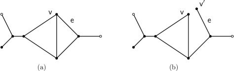
Figure 4.2. Disconnecting the edge $\mathsf{e}$ from the vertex $\mathsf{v}$ in the proof of Theorem 4.7. This operation reduces $\beta$ by 1 at the expense of increasing the number of Neumann vertices by 1.

Given a tree ${\mathcal{G}}$ we can find an arbitrarily small perturbation under which the $k$-th eigenvalue is simple and its eigenfunction is nonzero on vertices [BL17]. In these circumstances the $k$-th eigenfunction has exactly $k$ nodal domains [PPAO96, Sch06] (see also [BK12, Thm. 6.4] for a short proof). Each nodal domain is a subtree ${\mathcal{T}}_{j}$, and with vertex conditions inherited from ${\mathcal{G}}$ (plus Dirichlet conditions on the nodal domain boundaries), $\lambda_{k}({\mathcal{G}})$ is the first eigenvalue of the subtree.

There are at most $|N|$ subtrees with some Neumann conditions on their leaves. Since these are nodal subtrees ($k>1$), there are also some leaves with Dirichlet conditions and we can use estimate (4.3) in the form $L_{j}\sqrt{\lambda}\geq\pi/2$. The same conclusion is true if $k=1$ and ${\mathcal{G}}$ has at least one Dirichlet vertex.

If $k\geq|N|$, we also have at least $k-|N|$ subtrees with only Dirichlet conditions at the leaves, for which we can use the bound of Theorem 4.6 but with the diameter substituted by the total length of the subtree, i.e. $L_{j}\sqrt{\lambda}\geq(\operatorname{diam}{{\mathcal{T}}}_{j})\sqrt{\lambda}\geq\pi$. We therefore have

$$L\sqrt{\lambda_{k}({\mathcal{G}})}=\sum_{j=1}^{k}L_{j}\sqrt{\lambda_{1}({\mathcal{T}}_{j})}\geq|N|\frac{\pi}{2}+(k-|N|)\pi=\left(k-\tfrac{|N|}{2}\right)\pi.\$$

When $k<|N|$, we use estimate (4.3) for each of the $k$ nodal subtrees, obtaining Friedlander’s bound. ∎

4.3. Upper bound for all eigenvalues

We now slightly extend and improve the beautiful recent result of Ariturk [Ari16, Thm. 1.2], providing at the same time a simpler proof.

Theorem 4.9.

Let ${\mathcal{G}}$ be a connected quantum graph with Dirichlet or Neumann conditions at the vertices of degree one and natural condition elsewhere. If ${\mathcal{G}}$ is not a cycle, then for all $k\in\mathbb{N}$

(4.9) $$\lambda_{k}({\mathcal{G}})\leq\left(k-2+\beta+|D|+\tfrac{|N|+\beta}{2}\right)^{2}\frac{\pi^{2}}{L^{2}},$$

where the set of Dirichlet vertices is denoted by $D$ and the set of Neumann vertices of degree one is denoted by $N$.

Remark 4.10.

(a) Both Theorem 4.7 and Theorem 4.9 are false on cycle graphs. If ${\mathcal{G}}$ is a loop with a pendant edge attached to it (i.e., a “lollipop” or “lasso” graph), and with the Neumann condition at the pendant vertex, then Theorems 4.7 and 4.9 result in the two-sided bound

$$\frac{(k-1)^{2}\pi^{2}}{L^{2}}\leq\lambda_{k}(\mathcal{G})\leq\frac{k^{2}\pi^{2}}{L^{2}}$$

for $k\geq 2$ large enough. Remarkably, as the length of the pendant edge converges to zero, odd-numbered eigenvalues converge to the lower bound while even-numbered ones converge to the upper bound.

(b) Similarly to the bound of Theorem 4.7, the upper bound in (4.9) is asymptotically sharp. The only other asymptotically sharp bounds known to the authors is the one by Nicaise [Nic87, Th. 2.4], who proved that for equilateral graphs

(4.10) $$\frac{(k-1-L)^{2}\pi^{2}}{L^{2}}\leq\lambda_{k}({\mathcal{G}})\leq\frac{(k-1+L)^{2}\pi^{2}}{L^{2}}\ .$$

Under some circumstances (for example for complete graphs with many vertices), bound (4.10) is tighter than (4.9); informal scaling arguments suggest that, for large $\beta$, the factor in front of $\beta$ in (4.9) should be 1 instead of the current $\frac{3}{2}$ (see also the discussion following Theorem 1.2 in [Ari16]; note that in the results of [Ari16] the corresponding factor is 2).

Proof of Theorem 4.9.

If ${\mathcal{G}}$ is not a tree (i.e. if $\beta>0$) and not a cycle, we repeat the process described at the beginning of the proof of Theorem 4.7, disconnecting $\beta$ edges at vertices and creating a tree ${\mathcal{T}}$ with $\beta$ additional Neumann vertices of degree one. At every step, the eigenvalue goes down, but not further than the next eigenvalue (see [BK13, Thm 3.1.10]), therefore we have $\lambda_{k}({\mathcal{G}})\leq\lambda_{k+\beta}({\mathcal{T}})$ and the bound for general graphs follows from the bound for trees, $\beta=0$.

We will prove the result assuming ${\mathcal{G}}$ is a tree by induction on the number of edges. The inequality turns into equality for a single edge with either Dirichlet or Neumann or mixed conditions.

Choose an arbitrary vertex $\mathsf{v}$ of degree three or more and apply Lemma 4.1 (the third inequality) with $r=1$. Let ${\mathcal{G}}^{\prime}$ be the graph realizing this inequality; it is a disjoint union of two trees, denote them by ${\mathcal{T}}_{1}$ and ${\mathcal{T}}_{2}$. Without loss of generality, $\lambda_{k}({\mathcal{G}}^{\prime})$ is an eigenvalue of ${\mathcal{T}}_{1}$; denote its position in the spectrum of ${\mathcal{T}}_{1}$ by $j\leq k$. We therefore have

$$\lambda_{k}({\mathcal{G}}^{\prime})=\lambda_{j}({\mathcal{T}}_{1})\qquad\mbox{and}\qquad\lambda_{k}({\mathcal{G}}^{\prime})\leq\lambda_{k-j+1}({\mathcal{T}}_{2}).$$

Denoting by $L_{1}$ and $L_{2}$ the total lengths of the two trees, we have $L=L_{1}+L_{2}$. Denoting by $D_{1}$ and $D_{2}$ the Dirichlet vertices, we also have $|D|=|D_{1}|+|D_{2}|-1$, since one Dirichlet vertex was added in the process of application of Lemma 4.1 with $r=1$. We now use the inductive hypothesis for the two trees $T_{1}$ and $T_{2}$ to get

$$L\sqrt{\lambda_{k}({\mathcal{G}})} \leq L_{1}\sqrt{\lambda_{j}({\mathcal{T}}_{1})}+L_{2}\sqrt{\lambda_{k-j+1}({\mathcal{T}}_{2})}$$

$$\leq\pi\left(j-2+|D_{1}|+\tfrac{|N_{1}|}{2}\right)+\pi\left(k-j+1-2+|D_{2}|+\tfrac{|N_{2}|}{2}\right)$$

$$=\pi\left(k-3+|D|+1+\tfrac{|N|}{2}\right).$$

This completes the proof. ∎

4.4. Implications for the normalized and discrete Laplacians

It is known that formula (3.13) can be generalized to the higher eigenvalues: indeed, von Below has shown that

(4.11) $$\mu({\mathcal{G}})=\left(\arccos(1-\alpha(\mathsf{G}))\right)^{2},$$

cf. [Bel85, Thm. on p. 320], for all eigenvalues $0=\mu_{0}({\mathcal{G}})<\mu_{1}({\mathcal{G}})\leq\ldots$ of $\Delta$ within the interval $[0,\pi^{2}]$ and $0=\alpha_{0}(\mathsf{G})<\alpha_{1}(\mathsf{G})\leq\ldots\leq\alpha_{V-1}(\mathsf{G})$ of $\mathcal{L}_{\rm norm}$ within the interval $[0,2]$ (with the exception of $\mu=\pi^{2}$, which is an eigenvalue of $\Delta$ whenever $\mathsf{G}$ is a non-bipartite unicyclic graph although $2$ is not an eigenvalue of $\mathcal{L}_{\rm norm}$); also, the multiplicities coincide, so that in fact switching to the notation adopted in this section we can write

(4.12) $$\alpha_{k-1}(\mathsf{G})=1-\cos\sqrt{\lambda_{k}({\mathcal{G}})}\qquad\hbox{for all }k=1,\ldots,V\ .$$

Accordingly, all of our results in this section can be translated into both upper and lower estimates on all eigenvalues $\alpha_{k}(\mathsf{G})$ of normalized Laplacians and we obtain the following.

Proposition 4.11.

Let $\mathsf{G}$ be a connected combinatorial graph without loops, which has $V^{*}\geq 0$ vertices of degree $>1$. Then the eigenvalues $\alpha_{k}(\mathsf{G})$ of the normalized Laplacian on $\mathsf{G}$ satisfy, for all $k=2,\ldots,V$, the estimates

(4.13) $$1-\cos\left(\frac{2k-E+V^{*}-1}{2E}\cdot\pi\right)\leq\alpha_{k-1}(\mathsf{G}),$$

as well as

(4.14) $$1-\cos\frac{k\pi}{2E}\leq\alpha_{k-1}(\mathsf{G}),$$

and

(4.15) $$\alpha_{k-1}(\mathsf{G})\leq 1-\cos\left(\frac{2k+3E-V-V^{*}-1}{2E}\cdot\pi\right),$$

where (4.13) holds provided

(4.16) $$k\geq E-V^{*}+1$$

and (4.15) provided

(4.17) $$2k-V-V^{*}-1+E\leq 0.$$

Observe that conditions (4.16) and (4.17) imply in particular that the arguments of $\cos(\,\cdot\,)$ in (4.13) and (4.15) lie in $[0,\pi]$, the domain of monotonicity of $1-\cos(\,\cdot\,)$.

Example 4.12.

A necessary condition for the lower estimate to be nontrivial (i.e., to hold for at least one $k$) is that $V+V^{*}\geq E+1$: this is indeed satisfied for complete graphs $\mathsf{K}_{n}$ with $n\leq 4$ (since then $V+V^{*}=2n\geq\frac{n(n-1)}{2}+1=E+1$), cycle graphs $\mathsf{C}_{n}$ ($V+V^{*}=2n\geq n+1=E+1$), path graphs $\mathsf{P}_{n}$ ($V+V^{*}=2n-2\geq n=E+1$), star graphs $\mathsf{S}_{n+1}$ ($V+V^{*}=n+2\geq n+1=E+1$), wheel graphs $\mathsf{W}_{n+1}$ ($V+V^{*}=2n+2\geq 2n+1=E+1$, but for no complete bipartite graphs $\mathsf{K}_{n,m}$ with $n\neq 1\neq m$ ($V+V^{*}=n+m\not\geq nm+1=E+1$) and no nontrivial hypercube graphs $\mathsf{Q}_{n}$ ($V+V^{*}=2^{n+1}\not\geq 2^{n-1}n+1=E+1$).

In the case of star graphs $\mathsf{S}_{n+1}$ our lower estimate is sharp: it reads

$$1\leq\alpha_{n-1}(\mathsf{S}_{n+1}),$$

which delivers the actual value; whereas in the case of the wheel graph we find

$$0.293\simeq 1-\cos\frac{\pi}{4}\leq\alpha_{n-1}(\mathsf{W}_{n+1}),$$

to be compared with the actual value of $1-\frac{2}{3}\cos\frac{2\pi(n-1)}{n}\to\frac{1}{3}$ as $n\to\infty$.

Our upper estimate cannot be applied unless condition (4.17) is satisfied: this actually fails in the case of star graphs, wheel graphs, complete graphs or nontrivial hypercube graphs, for which we cannot improve the trivial upper estimate $\alpha_{k}\leq 2$ for all $k$. In most cases where condition (4.17) does hold, like the Petersen graph (for $k=2,3$), path graphs $\mathsf{P}_{n}$ (for $2\leq k\leq\frac{n}{2}$), complete bipartite graphs $\mathsf{K}_{n,m}$ (for $k\leq n+m-\frac{1}{2}(mn-1)$) or cycle graphs $\mathsf{C}_{n}$ (for $2\leq k\leq\frac{n+1}{2}$), the upper estimates are however typically much rougher than the corresponding lower estimates; this seems to substantiate our conjecture in Remark 4.10.

In view of the version of (3.14) for the higher eigenvalues, namely

(4.18) $$\alpha_{k}(\mathsf{G})\deg_{\rm max}(\mathsf{G})\geq\gamma_{k}(\mathsf{G})\geq\alpha_{k}(\mathsf{G})\deg_{\rm min}(\mathsf{G})\ ,$$

analogous estimates hold also for the eigenvalues of the discrete Laplacian $\mathcal{L}$. We are not aware of any earlier result of this kind in the literature about discrete and normalized Laplacians, apart from the trivial estimate $\alpha_{\max}(\mathsf{G})\leq 2$ and the estimates on $\gamma_{\max}(\mathsf{G})$ summarized in [LZ98, Shi07].

References

- [Ari16] S. Ariturk. Eigenvalue estimates on quantum graphs. Preprint arXiv:1609.07471, 2016.
- [BBW15] R. Band, G. Berkolaiko, and T. Weyand. Anomalous nodal count and singularities in the dispersion relation of honeycomb graphs. J. Math. Phys., 56(12):122111, 2015.
- [Bel85] J. von Below. A characteristic equation associated to an eigenvalue problem on -networks. Linear Algebra Appl., 71:309–325, 1985.
- [Ber16] G. Berkolaiko. Elementary introduction to quantum graphs. Preprint arXiv:1603.07356 [math-ph], 2016.
- [BH09] T. Bühler and M. Hein. Spectral clustering based on the graph -Laplacian. In Proc. 26th Annual Int. Conf. Mach. Learning, pages 81–88. ACM, New York, 2009.
- [BK12] G. Berkolaiko and P. Kuchment. Dependence of the spectrum of a quantum graph on vertex conditions and edge lengths. In Spectral Geometry, volume 84 of Proceedings of Symposia in Pure Mathematics. American Math. Soc., 2012. Preprint arXiv:1008.0369.
- [BK13] G. Berkolaiko and P. Kuchment. Introduction to Quantum Graphs, volume 186 of Mathematical Surveys and Monographs. AMS, 2013.
- [BL16] R. Band and G. Lévy. Quantum graphs which optimize the spectral gap. Preprint arXiv:1608.00520, 2016.
- [BL17] G. Berkolaiko and W. Liu. Simplicity of eigenvalues and non-vanishing of eigenfunctions of a quantum graph. J. Math. Anal. Appl., 445(1):803–818, 2017. Preprint arXiv:1601.06225.
- [Bol98] B. Bollobás. Modern graph theory, volume 184 of Graduate Texts in Mathematics. Springer-Verlag, New York, 1998.
- [BR08] P.A. Binding and R.P. Rynne. Variational and non-variational eigenvalues of the -laplacian. J. Differential Equations, 244:24–39, 2008.
- [But08] S.K. Butler. Eigenvalues and Structures of Graphs. PhD thesis, University of California, San Diego, 2008.
- [Chu97] F.R.K. Chung. Spectral graph theory, volume 92 of CBMS Regional Conference Series in Mathematics. Published for the Conference Board of the Mathematical Sciences, Washington, DC, 1997.
- [DPR16] L.M. Del Pezzo and J.D. Rossi. The first eigenvalue of the -Laplacian on quantum graphs. Anal. Math. Phys., 6(4):365–391, 2016.
- [Fie73] M. Fiedler. Algebraic connectivity of graphs. Czechoslovak Math. J., 23(98):298–305, 1973.
- [Fri05] L. Friedlander. Extremal properties of eigenvalues for a metric graph. Ann. Inst. Fourier (Grenoble), 55(1):199–211, 2005.
- [GS06] S. Gnutzmann and U. Smilansky. Quantum graphs: Applications to quantum chaos and universal spectral statistics. Adv. Phys., 55(5–6):527–625, 2006.
- [HLM15] M. Hein, D. Lenz and D. Mugnolo (eds.). Mini-workshop: Discrete -laplacians: Spectral theory and variational methods in mathematics and computer science. Oberwolfach Reports, 12(1):399–447, 2015.
- [KKMM16] J.B. Kennedy, P. Kurasov, G. Malenová and D. Mugnolo. On the spectral gap of a quantum graph. Ann. Henri Poincaré, 17(9):2439–2473, 2016.
- [KMN13] P. Kurasov, G. Malenová and S. Naboko. Spectral gap for quantum graphs and their edge connectivity. J. Phys. A, 46(27):275309, 16, 2013.
- [KN14] P. Kurasov and S. Naboko. Rayleigh estimates for differential operators on graphs. J. Spectr. Theory, 4(2):211–219, 2014.
- [LE11] J. Lang and D. Edmunds. Eigenvalues, embeddings and generalised trigonometric functions, volume 2016 of Lecture Notes in Mathematics. Springer, Heidelberg, 2011.
- [LZ98] J.-S. Li and X.-D. Zhang. On the Laplacian eigenvalues of a graph. Lin. Algebra Appl., 285:305–307, 1998.
- [Mug13] D. Mugnolo. Parabolic theory of the discrete -Laplace operator. Nonlinear Anal., 87:33–60, 2013.
- [Mug14] D. Mugnolo. Semigroup methods for evolution equations on networks. Understanding Complex Systems. Springer, Cham, 2014.
- [Nic87] S. Nicaise. Spectre des réseaux topologiques finis. Bull. Sci. Math. (2), 111(4):401–413, 1987.
- [NY76] T. Nakamura and M. Yamasaki. Generalized extremal length of an infinite network. Hiroshima Math. J., 6(1):95–111, 1976.
- [PPAO96] Yu.V. Pokornyĭ, V.L. Pryadiev and A. Al′-Obeĭd. On the oscillation of the spectrum of a boundary value problem on a graph. Mat. Zametki, 60(3):468–470, 1996.
- [Roh16] J. Rohleder. Eigenvalue estimates for the laplacian on a metric tree. Proc. Amer. Math. Soc., 2016. To appear.
- [Sch06] P. Schapotschnikow. Eigenvalue and nodal properties on quantum graph trees. Waves Random Complex Media, 16(3):167–178, 2006.
- [Shi07] L. Shi. Bounds on the (Laplacian) spectral radius of graphs. Lin. Algebra Appl., 422:755–770, 2007.
- [Spi09] D. Spielman. Spectral graph theory — Manuscript of a Yale course (appl. math. 561/comp. sci. 662). Available at http://www.cs.yale.edu/homes/spielman/561/2009/lect02-09.pdf, 2009.