Gaussian and Sparse Processes Are Limits of Generalized Poisson Processes

Abstract

The theory of sparse stochastic processes offers a broad class of statistical models to study signals. In this framework, signals are represented as realizations of random processes that are solution of linear stochastic differential equations driven by white Lévy noises. Among these processes, generalized Poisson processes based on compound-Poisson noises admit an interpretation as random $\mathrm{L}$-splines with random knots and weights. We demonstrate that every generalized Lévy process—from Gaussian to sparse—can be understood as the limit in law of a sequence of generalized Poisson processes. This enables a new conceptual understanding of sparse processes and suggests simple algorithms for the numerical generation of such objects.

I Introduction

In their landmark paper on linear prediction [1], H. W. Bode and C. E. Shannon proposed that “a (…) noise can be thought of as made up of a large number of closely spaced and very short impulses." In this work, we formulate this intuitive interpretation of a white noise in a mathematically rigorous way. This allows us to extend this intuition beyond noise and to draw additional properties for the class of stochastic processes that can be linearly transformed into a white noise. More precisely, we show that the law of these processes can be approximated as closely as desired by generalized Poisson processes that can also be viewed as random $\mathrm{L}$-splines.

Let us define the first ingredient of our work. Splines are continuous-domain functions characterized by a sequence of knots and sample values. They provide a powerful framework to build discrete descriptions of continuous objets in sampling theory [2]. Initially defined as piecewise-polynomial functions [3], they were further generalized, starting from their connection with differential operators [4, 5, 6]. Let $\mathrm{L}$ be a suitable linear differential operator such as the derivative. Then, the function $s:\mathbb{R}^{d}\rightarrow\mathbb{R}$ is a non-uniform $\mathrm{L}$-spline if

$$\mathrm{L}s=\sum_{k=0}^{\infty}a_{k}\delta(\cdot-\bm{x}_{k}):=w_{\delta}$$ (1)

is a sum of weighted and shifted Dirac impulses. The $a_{k}$ are the weights and the $\bm{x}_{k}$ the knots of the spline. Deterministic splines associated to various differential operators are depicted in Figure 1. Note that the knots $\bm{x}_{k}$ and weights $a_{k}$ can also be random, yielding stochastic splines.

The second main ingredient is a generative model of stochastic processes. Specifically, we consider linear differential equations of the form

$$\mathrm{L}s=w,$$ (2)

where $\mathrm{L}$ is a differential operator called the whitening operator and $w$ is a $d$-dimensional Lévy noise or innovation. Examples of such stochastic processes are illustrated in Figure 2.

Our goal in this paper is to build a bridge between linear stochastic differential equations (linear SDE) and splines. By comparing (1) and (2), one easily realizes that the differential operator $\mathrm{L}$ connects the random and deterministic frameworks. The link is even stronger when one notices that compound-Poisson white noises can be written as $w_{\mathrm{Poisson}}=w_{\delta}$ [7]. This means that the random processes that are solution of $\mathrm{L}s=w_{\mathrm{Poisson}}=w_{\delta}$ are (random) $\mathrm{L}$-splines.

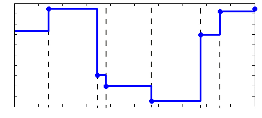
(a)

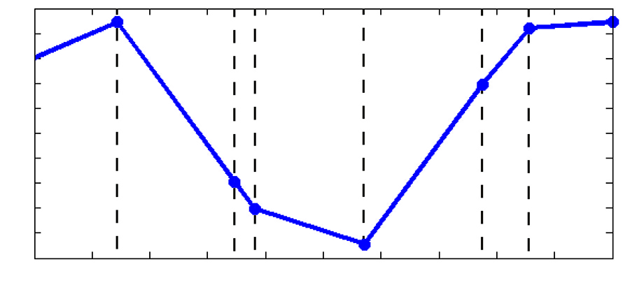
(b)

Figure 1: Examples of deterministic splines: (a) piecewise constant, (b) piecewise linear.

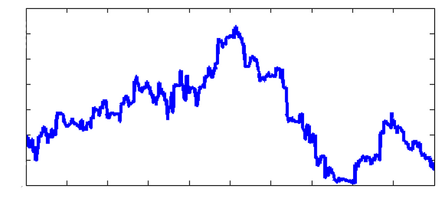
(a)

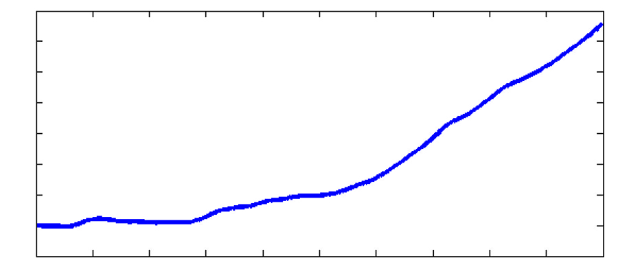
(b)

Figure 2: Examples of random processes: (a) Brownian motion, (b) second-order Gaussian process.

Our main result thus uncovers the link between splines and random processes through the use of Poisson processes. A Poisson noise is made of a sparse sequence of weighted impulses whose jumps follow a common law. The average density of impulses $\lambda$ is the primary parameter of such a Poisson white noise: Upon increasing $\lambda$, one increases the average number of impulses by unit of time. Meanwhile, the intensity of the impulses is governed by the common law of the jumps of the noise: Upon decreasing this intensity, one makes the weights of the impulses smaller. By combining these two effects, one can recover the intuitive conceptualization of a white noise proposed by Bode and Shannon in [1].

Theorem 1.

Every random process $s$ solution of (2) is the limit in law of the sequence $(s_{n})$ of generalized Poisson processes driven by compound-Poisson white noises and whitened by $\mathrm{L}$.

We shall see that the convergence procedure is based on a coupled increase of the average density and a decrease of the intensity of the impulses of the Poisson noises. This is in the spirit of Bode and Shannon’s quote and is, in fact, true for any Lévy noise.

I-A Connection with Related Works

Random processes and random fields are notorious tools to model uncertainty and statistics of signals [8]. Gaussian processes are by far the most studied stochastic models because of their fundamental properties (e.g., stability, finite variance, central-limit theorem) and their relative ease of use. They are the principal actors within the “classical” paradigm in statistical signal processing [9]. Many fractal-type signals are modeled as self-similar Gaussian processes [10, 11, 12, 13]. However, many real-world signals are empirically observed to be inherently sparse, a property that is incompatible with Gaussianity [14, 15, 16]. In order to overcome the limitations of Gaussian model, several other stochastic models has been proposed for the study of sparse signals. They include infinite-variance [12, 17] or piecewise-constant models [14, 7].

In this paper, we model signals as continuous-domain random processes defined over $\mathbb{R}^{d}$ that are solution of a differential equation driven by Lévy noise. These processes are called generalized Lévy processes. We thus follow the general approach of [9] which includes the models mentioned above. The common feature of these processes is that their probability distributions are always infinitely divisible, meaning that they can be decomposed as sums of any length of independent and identically distributed random variables. Infinite divisibility is a key concept of continuous-domain random processes [18] and will be at the heart of our work. In order to embrace the largest variety of random models, we rely on the framework of generalized random processes, which is the probabilistic version of the theory of generalized functions of L. Schwartz [19]. Initially introduced independently by K. Itō [20] and I. Gelfand [21], it has been developed extensively by these two authors in [22] and [23].

Several behaviors can be observed within this extended family of random processes. For instance, self-similar Gaussian processes exhibit fractal behaviors. In one dimension, they include the fractional Brownian motion [10] and its higher-order extensions [24]. In higher dimensions, our framework covers the family of fractional Gaussian fields [25, 26, 27] and finite-variance self-similar fields that appear to converge to fractional Gaussian fields at large scales [28]. The self-similarity property is also compatible with the family of $\alpha$-stable processes [29] which have the particularity of having unbounded variances or second-order moments (when non-Gaussian). More generally, every process considered in our framework is part of the Lévy family, including Laplace processes [30] and Student’s processes [31]. Upon varying the operator $\mathrm{L}$, one recovers Lévy processes [32], CARMA processes [33, 34], and their multivariate generalizations [9, 35]. Unlike those examples, the compound-Poisson processes, although members of the Lévy family, are piecewise-constant and have a finite rate of innovation (FRI) in the sense of [36]. For a signal, being FRI means that a finite quantity of information is sufficient to reconstruct it over a bounded domain.

The present paper is an extension of our previous contribution [37]. We believe that Theorem 1 is relevant for the conceptualization of random processes that are solution of linear SDE. Starting from the $\mathrm{L}$-spline interpretation of generalized Poisson processes, the statistics of a more general process can be understood as a limit of the statistics of random $\mathrm{L}$-splines. In general, the studied processes that are solution of (2) do not have a finite rate of innovation, unless the underlying white noise is Poisson. The convergence result helps us understand why non-Poisson processes do not have a finite rate of innovation: They correspond to infinitely many impulses per unit of time as they can be approximated by FRI processes with an increasing and asymptotically infinite rate of innovation.

Interesting connections can also be drawn with some classical finite-dimension convergence results in probability theory. As mentioned earlier, there is a direct correspondence between Lévy white noises and infinitely divisible random variables. It is well known that any infinitely divisible random variable is the limit in law of a sequence of compound-Poisson random variables [18, Corollary 8.8]). Theorem 1 is the generalization of this result from real random variables to random processes that are solution of a linear SDE.

I-B Outline

The paper is organized as follows: In Sections II and  III, we introduce the concepts of $\mathrm{L}$-splines and generalized Lévy processes, respectively. A special emphasis on generalized Poisson processes is given in Section IV as they both embrace generalized Lévy processes and (random) $\mathrm{L}$-splines. Our main contribution is Theorem 1; it is proven in Section V. Section VI contains illustrative examples in the one- and two-dimensional settings, followed by concluding remarks in Section VII.

II Nonuniform $\mathrm{L}$-Splines

We denote by ${\mathcal{S}}(\mathbb{R}^{d})$ the space of rapidly decaying functions from $\mathbb{R}^{d}$ to $\mathbb{R}$. Its topological dual is ${\mathcal{S}}^{\prime}(\mathbb{R}^{d})$, the Schwartz space of tempered generalized function [19]. We denote by $\langle u,\varphi\rangle$ the duality product between $u\in{\mathcal{S}}^{\prime}(\mathbb{R}^{d})$ and $\varphi\in{\mathcal{S}}(\mathbb{R}^{d})$. A linear and continuous operator $\mathrm{L}$ from ${\mathcal{S}}(\mathbb{R}^{d})$ to ${\mathcal{S}}^{\prime}(\mathbb{R}^{d})$ is spline-admissible if

• it is shift-invariant, meaning that

  $$\mathrm{L}\{\varphi(\cdot-\bm{x}_{0})\}=\mathrm{L}\{\varphi\}(\cdot-\bm{x}_{0})$$ (3)

  for every $\varphi\in{\mathcal{S}}(\mathbb{R}^{d})$ and $\bm{x}_{0}\in\mathbb{R}^{d}$; and

• there exists a measurable function of slow growth $\rho_{\mathrm{L}}$ such that

  $$\mathrm{L}\{\rho_{\mathrm{L}}\}=\delta$$ (4)

  with $\delta$ the Dirac delta function. The function $\rho_{\mathrm{L}}$ is a Green’s function of $\mathrm{L}$.

Definition 1.

Let $\mathrm{L}$ be a spline-admissible operator with measurable Green’s function $\rho_{\mathrm{L}}$. A nonuniform $\mathrm{L}$-spline with knots $(\bm{x}_{k})$ and weights $(a_{k})$ is a function $s$ such that

$$\mathrm{L}s=\sum_{k=0}^{\infty}a_{k}\delta(\cdot-\bm{x}_{k}).$$ (5)

Definition 1 implies that the generic expression for a nonuniform $\mathrm{L}$-spline is

$$s=p_{0}+\sum_{k\in\mathbb{Z}}a_{k}\rho_{\mathrm{L}}(\cdot-\bm{x}_{k})$$ (6)

with $p_{0}$ in the null space of $\mathrm{L}$ (i.e., $\mathrm{L}p_{0}=0$). Indeed, we have, by linearity and shift-invariance of $\mathrm{L}$, that

$$\mathrm{L}\Big{\{}s-\sum_{k\in\mathbb{Z}}a_{k}\rho_{\mathrm{L}}(\cdot-\bm{x}_{k})\Big{\}}=\mathrm{L}s-\sum_{k\in\mathbb{Z}}a_{k}\delta(\cdot-\bm{x}_{k})=0.$$ (7)

Therefore, $\left(s-\sum_{k\in\mathbb{Z}}a_{k}\rho_{\mathrm{L}}(\cdot-\bm{x}_{k})\right)$ is in the null space of $\mathrm{L}$.

TABLE I: Some families of spline-admissible operators

Dimension	Operator	Parameter	$\rho_{\mathrm{L}}(\bm{x})$	Spline type	References
1	$\mathrm{D}^{N}$	$N\in\mathbb{N}\backslash\{0\}$	$\frac{1}{(N-1)!}x^{N-1}u(x)$	B-splines	[2, 3]
1	$(\mathrm{D}+\alpha\mathrm{I})$	$\alpha\in\mathbb{C},\Re(\alpha)>0$	$\mathrm{e}^{-\alpha x}u(x)$	E-splines	[38]
1	$\mathrm{D}^{\gamma}$	$\gamma>0$	$\frac{1}{\Gamma(\gamma)}x^{\gamma-1}u(x)$	fractional splines	[6, 39]
$d$	$\mathrm{D}_{x_{1}}\cdots\mathrm{D}_{x_{d}}$	-	$u(\bm{x})=\prod_{i=1}^{d}u(x_{i})$	separable splines	[9]
$d$	$(-\Delta)^{m/2}$	$m-d\in 2\mathbb{N}$	$c_{m,d}\lVert\bm{x}\rVert^{m-d}\log\lVert\bm{x}\rVert$	cardinal polyharmonic splines	[5]
$d$	$(-\Delta)^{\gamma/2}$	$\gamma-d\in\mathbb{R}^{+}\backslash 2\mathbb{N}$	$c_{\gamma,d}\lVert\bm{x}\rVert^{\gamma-d}$	fractional polyharmonic splines	[40]

We summarize in Table I important families of operators with their corresponding Green’s function and the associated family of $\mathrm{L}$-splines. The Heaviside function is denoted by $u$. The large variety of proposed splines illustrates the generality of our result.

III Generalized Lévy Processes

In this section, we briefly introduce the main tools and concepts for the characterization of sparse processes. For a more comprehensive description, we refer the reader to [9]. First, let us recall that a real random variable $X$ is a measurable function from a probability space $(\Omega,\mathcal{A},\mathscr{P})$ to $\mathbb{R}$, endowed with the Borelian $\sigma$-field. The law of $X$ is the probability measure on $\mathbb{R}$ such that $\mathscr{P}_{X}([a,b])=\mathscr{P}(a\leq X(\omega)\leq b)$. The characteristic function of $X$ is the (conjugate) Fourier transform of $\mathscr{P}$. For $\xi\in\mathbb{R}$, it is

$${\widehat{\mathscr{P}}}_{X}(\xi)=\int_{\mathbb{R}}\mathrm{e}^{\mathrm{i}\xi x}\mathrm{d}\mathscr{P}_{X}(x)=\mathbb{E}[\mathrm{e}^{\mathrm{i}X\xi}].$$ (8)

III-A Generalized Random Processes

Generalized Lévy processes are defined in the framework of generalized random processes [22], which is the stochastic counterpart of the theory of generalized functions.

III-A1 Random Elements in ${\mathcal{S}}^{\prime}(\mathbb{R}^{d})$

We first define the cylindrical $\sigma$-field on the Schwartz space ${\mathcal{S}}^{\prime}(\mathbb{R}^{d})$, denoted by $\mathcal{B}_{c}({\mathcal{S}}^{\prime}(\mathbb{R}^{d}))$, as the $\sigma$-field generated by the cylinders

$$\left\{v\in{\mathcal{S}}^{\prime}(\mathbb{R}^{d}),\quad(\langle v,\varphi_{1}\rangle,\ldots,\langle v,\varphi_{N}\rangle)\in B\right\},$$ (9)

where $N\geq 1$, $\varphi_{1},\ldots,\varphi_{N}\in{\mathcal{S}}(\mathbb{R}^{d})$, and $B$ is a Borelian subset of $\mathbb{R}^{N}$.

Definition 2.

A generalized random process is the measurable function

$$s\ :\ (\Omega,\mathcal{A})\rightarrow({\mathcal{S}}^{\prime}(\mathbb{R}^{d}),\mathcal{B}_{c}({\mathcal{S}}^{\prime}(\mathbb{R}^{d}))).$$ (10)

The law of $s$ is then the probability measure $\mathscr{P}_{s}$ on ${\mathcal{S}}^{\prime}(\mathbb{R}^{d})$, image of $\mathscr{P}$ by $s$. The characteristic functional of $s$ is the Fourier transform of its probability law, defined for $\varphi\in{\mathcal{S}}(\mathbb{R}^{d})$ by

$${\widehat{\mathscr{P}}}_{s}(\varphi)=\int_{{\mathcal{S}}^{\prime}(\mathbb{R}^{d})}\mathrm{e}^{\mathrm{i}\langle v,\varphi\rangle}\mathrm{d}\mathscr{P}_{s}(v)=\mathbb{E}[\mathrm{e}^{\mathrm{i}\langle s,\varphi\rangle}].$$ (11)

A generalized process $s$ is therefore a random element in ${\mathcal{S}}^{\prime}(\mathbb{R}^{d})$. In particular, we have that

• for every $\omega\in\Omega$, the functional $\varphi\mapsto\langle s(\omega),\varphi\rangle$ is in ${\mathcal{S}}^{\prime}(\mathbb{R}^{d})$; and

• for every $\varphi_{1},\ldots\varphi_{N}\in{\mathcal{S}}(\mathbb{R}^{d})$,

  $$\omega\mapsto\bm{Y}=\left(\langle s(\omega),\varphi_{1}\rangle,\ldots,\langle s(\omega),\varphi_{N}\rangle\right)$$ (12)

  is a random vector whose characteristic functions

  $${\widehat{\mathscr{P}}}_{\bm{Y}}(\bm{\xi})={\widehat{\mathscr{P}}}_{s}(\xi_{1}\varphi_{1}+\cdots+\xi_{N}\varphi_{N})$$ (13)

  for every $\bm{\xi}=(\xi_{1},\ldots,\xi_{N})\in\mathbb{R}^{N}$.

The probability density functions (pdfs) of the random vectors $\bm{Y}$ in (12) are the finite-dimensional marginals of $s$. We shall omit the reference to $\omega\in\Omega$ thereafter.

III-A2 Abstract Nuclear Spaces

We recall that function spaces are locally convex spaces, generally infinite-dimensional, whose elements are functions. To quote A. Pietsch in [41]: “The locally convex spaces encountered in analysis can be divided into two classes. First, there are the normed spaces (…). The second class consists of the so-called nuclear locally convex spaces." Normed spaces and nuclear spaces are mutually exclusive in infinite dimension [42, Corollary 2, pp. 520]. The typical example of nuclear function space is the Schwartz space ${\mathcal{S}}(\mathbb{R}^{d})$ [42, Corollary, pp. 530]; see also [23].

The theory of nuclear spaces was introduced by A. Grothendieck in [43]. The required formalism is more demanding than the simpler theory of Banach spaces. The payoff is that fundamental results of finite-dimensional probability theory can be directly extended to nuclear spaces, while such generalizations are not straightforward for Banach spaces.

Let $\mathcal{N}$ be a nuclear space and $\mathcal{N}^{\prime}$ its topological dual. As we did for ${\mathcal{S}}^{\prime}(\mathbb{R}^{d})$ in Section III-A1, we define a generalized random process on $\mathcal{N}$ as a random variable $s$ from $\Omega$ to $\mathcal{N}^{\prime}$, endowed with the cylindrical $\sigma$-field $\mathcal{B}_{c}(\mathcal{N}^{\prime})$. The law of $s$ is the image of $\mathscr{P}$ by $s$ and is a probability measure on $\mathcal{N}^{\prime}$. The characteristic functional of $s$ is ${\widehat{\mathscr{P}}}_{s}(\varphi)=\mathbb{E}[\mathrm{e}^{\mathrm{i}\langle s,\varphi\rangle}]$, defined for $\varphi\in\mathcal{N}$.

III-A3 Generalized Bochner and Lévy Theorems

First, we recall the two fundamental theorems that support the use of the characteristic function in probability theory.

Proposition 1 (Bochner theorem).

A function ${\widehat{\mathscr{P}}}:\mathbb{R}\rightarrow\mathbb{C}$ is the characteristic function of some random variable $X$ if and only if ${\widehat{\mathscr{P}}}$ is continuous, positive-definite, and satisfies

$${\widehat{\mathscr{P}}}(0)=1.$$ (14)

Proposition 2 (Lévy theorem).

Let $(X_{n})_{n\in\mathbb{N}}$ and $X$ be real random variables. The sequence $X_{n}$ converges in law to $X$ if and only if for all $\xi\in\mathbb{R}$

$${\widehat{\mathscr{P}}}_{X_{n}}(\xi)\underset{n\rightarrow\infty}{\longrightarrow}{\widehat{\mathscr{P}}}_{X}(\xi),$$ (15)

where ${\widehat{\mathscr{P}}}_{X_{n}}$ and ${\widehat{\mathscr{P}}}_{X}$ are respectively the characteristic functions of $X_{n}$ and $X$.

The infinite-dimensional generalizations of Propositions 1 and 2 were achieved during the 60s and the 70s, and are effective for nuclear spaces only. See the introduction of [44] for a general discussion on this subject.

Initially conjectured by Gelfand, the so-called Minlos-Bochner theorem was proved by Minlos [45]. See also [22, Theorem 3, Section III-2.6].

Theorem 2 (Minlos-Bochner theorem).

Let $\mathcal{N}$ be a nuclear space. The functional ${\widehat{\mathscr{P}}}$ from $\mathcal{N}$ to $\mathbb{C}$ is the characteristic functional of a generalized random process $s$ on $\mathcal{N}^{\prime}$ if and only if ${\widehat{\mathscr{P}}}$ is continuous, positive-definite, and satisfies

$${\widehat{\mathscr{P}}}(0)=1.$$ (16)

The generalization of the Lévy theorem for nuclear spaces was obtained in [46, Theorem III.6.5] and is not as widely known as it should be. A sequence $(s_{n})_{n\in\mathbb{N}}$ of generalized random processes in $\mathcal{N}^{\prime}$ is said to converge in law to $s$, which we denote by $s_{n}\overset{(d)}{\underset{n\rightarrow\infty}{\longrightarrow}}s$ , if the underlying probability measures ${\widehat{\mathscr{P}}}_{s_{n}}$ converge weakly to ${\widehat{\mathscr{P}}}_{s}$, in such a way that

$$\int_{{\mathcal{S}}^{\prime}(\mathbb{R}^{d})}f(v)\mathrm{d}{\widehat{\mathscr{P}}}_{s_{n}}(v)\underset{n\rightarrow\infty}{\longrightarrow}\int_{{\mathcal{S}}^{\prime}(\mathbb{R}^{d})}f(v)\mathrm{d}{\widehat{\mathscr{P}}}_{s}(v)$$ (17)

for any continuous bounded function $f:{\mathcal{S}}^{\prime}(\mathbb{R}^{d})\rightarrow\mathbb{R}$.

Theorem 3 (Fernique-Lévy theorem).

Let $\mathcal{N}$ be a nuclear space. Let $(s_{n})_{n\in\mathbb{N}}$ and $s$ be generalized random processes on $\mathcal{N}^{\prime}$. Then, $s_{n}\overset{(d)}{\underset{n\rightarrow\infty}{\longrightarrow}}s$ if and only if the underlying characteristic functionals of $s_{n}$ converge pointwise to the characteristic functional of $s$, so that

$${\widehat{\mathscr{P}}}_{s_{n}}(\varphi)\underset{n\rightarrow\infty}{\longrightarrow}{\widehat{\mathscr{P}}}_{s}(\varphi)$$ (18)

for all $\varphi\in\mathcal{N}$.

Interestingly, it also appears that nuclear spaces are the unique Fréchet spaces for which the Lévy theorem still holds [47, Theorem 5.3].

We shall use Theorems 2 and 3 with $\mathcal{N}=\mathcal{S}(\mathbb{R}^{d})$. Theorem 2 is our main tool to construct solutions of stochastic differential equations as generalized random processes. On the other hand, Theorem 3 allows one to show the convergence in law of a family of generalized random processes.

III-B Lévy White Noises and generalized Lévy Processes

White noises can only be defined as generalized random processes, since they are too erratic to be defined as classical, pointwise processes.

III-B1 Lévy Exponents

Lévy white noises are in a one-to-one correspondence with infinitely divisible random variables. A random variable $X$ is said to be infinitely divisible if it can be decomposed for every $N\geq 1$ as

$$X=X_{1}+\cdots+X_{N},$$ (19)

where the $X_{n}$ are independent and identically distributed (i.i.d.) The characteristic function of an infinitely divisible law has the particularity of having no zero [18, Lemma 7.5], and therefore can be written as ${\widehat{\mathscr{P}}}_{X}(\xi)=\exp(f(\omega))$ with $f$ a continuous function [18, Lemma 7.6].

Definition 3.

A Lévy exponent is a function $f:\mathbb{R}\rightarrow\mathbb{C}$ that is the continuous log-characteristic function of an infinitely divisible law.

Theorem 4 gives the fundamental decomposition of a Lévy exponent. It is proved in [18, Section 8].

Theorem 4 (Lévy-Khintchine theorem).

A function $f:\mathbb{R}\rightarrow\mathbb{C}$ is a Lévy exponent if and only if it can be written as

$$f(\xi)=\mathrm{i}\mu\xi-\frac{\sigma^{2}\xi^{2}}{2}+\int_{\mathbb{R}}(\mathrm{e}^{\mathrm{i}\xi t}-1-\mathrm{i}\xi t1_{\lvert t\rvert\leq 1})V(\mathrm{d}t),$$ (20)

where $\mu\in\mathbb{R}$, $\sigma^{2}\geq 0$, and $V$ is a Lévy measure, which is a measure on $\mathbb{R}$ with

$$\int_{\mathbb{R}}\min(1,t^{2})V(\mathrm{d}t)<\infty\ \mbox{and}\ V(\{0\})=0.$$ (21)

We call $(\mu,\sigma^{2},V)$ the Lévy triplet associated to $f(\xi)$. If, moreover, one has that

$$\int_{\lvert t\rvert\geq 1}\lvert t\rvert^{\epsilon}V(\mathrm{d}t)<\infty$$ (22)

for some $\epsilon>0$, then $V$ is called a Lévy-Schwartz measure and one says that $f$ satisfies the Schwartz condition.

III-B2 Lévy White Noises

If $f$ is a Lévy exponent satisfying the Schwartz condition, then the functional

$$\varphi\mapsto\exp\left(\int_{\mathbb{R}^{d}}f(\varphi(\bm{x}))\mathrm{d}\bm{x}\right)$$ (23)

is a valid characteristic functional on ${\mathcal{S}}(\mathbb{R}^{d})$ [48, Theorem 3]. Hence, as a consequence of Theorem 2, there exists a generalized random process having this characteristic functional.

Definition 4.

A Lévy white noise on ${\mathcal{S}}^{\prime}(\mathbb{R}^{d})$ is the generalized random process $w$ whose characteristic functional has the form

$${\widehat{\mathscr{P}}}_{w}(\varphi)=\exp\left(\int_{\mathbb{R}^{d}}f(\varphi(\bm{x}))\mathrm{d}\bm{x}\right),$$ (24)

where $f$ is a Lévy exponent satisfying the Schwartz condition.

Lévy white noises are stationary, meaning that $w(\cdot-\bm{x}_{0})$ and $w$ have the same probability law for every $\bm{x}_{0}$. They are, moreover, independent at every point, in the sense that $\langle w,\varphi_{1}\rangle$ and $\langle w,\varphi_{2}\rangle$ are independent if $\varphi_{1}$ and $\varphi_{2}$ have disjoint supports.

III-B3 Generalized Lévy Processes

We want to define random processes $s$ solutions of the equation $\mathrm{L}s=w$. This requires one to identify compatibility conditions between $\mathrm{L}$ and $w$. This question was addressed in previous works [9, 48, 49] that we summarize now.

Definition 5.

Let $(\mu,\sigma^{2},V)$ be a Lévy triplet. For $0\leq p_{\min}\leq p_{\max}\leq 2$, one says that $(\mu,\sigma^{2},V)$ is a $(p_{\min},p_{\max})$-triplet if there exists

$$p_{\min}\leq p\leq q\leq p_{\max}$$ (25)

such that

1. $\int_{|t|\geq 1}\lvert t\rvert^{p}V(\mathrm{d}t)<\infty$,

2. $\int_{|t|<1}\lvert t\rvert^{q}V(\mathrm{d}t)<\infty$,

3. $p_{\min}=\inf(p,1)$ if $V$ is non-symmetric or $\mu\neq 0$, and

4. $p_{\max}=2$ if $\sigma^{2}\neq 2$.

If $f$ is the Lévy exponent associated to $(\mu,\sigma^{2},V)$, then one also says that $f$ is a $(p_{\min},p_{\max})$-exponent.

If $V$ is symmetric, then $(0,0,V)$ is a $(p_{\min},p_{\max})$-triplet if and only if

$$\int_{|t|\geq 1}\lvert t\rvert^{p_{\min}}V(\mathrm{d}t)\ \mbox{and}\ \int_{|t|<1}\lvert t\rvert^{p_{\max}}V(\mathrm{d}t)<\infty.$$ (26)

The other conditions are added to deal with the presence of a Gaussian part (for which $p_{\max}=2$) and the existence of asymmetry (for which $p_{\min}\geq 1$). Note, moreover, that every Lévy exponent is a $(0,2)$-exponent and that a Lévy exponent satisfies the Schwartz condition if and only if it is an $(\epsilon,2)$-exponent for some $0<\epsilon\leq 2$.

Definition 6.

Let $\mathrm{L}$ be a spline-admissible operator and $w$ a Lévy white noise with Lévy exponent $f$. One says that $(\mathrm{L},w)$ is compatible if there exists

$$0<p_{\min}\leq p_{\max}\leq 2$$ (27)

such that

• the function $f$ is a $(p_{\min},p_{\max})$-exponent; and

• the adjoint $\mathrm{L}^{*}$ of $\mathrm{L}$ admits a left inverse $\mathrm{T}$ such that

  $$\mathrm{T}\mathrm{L}^{*}\{\varphi\}=\varphi,\quad\forall\varphi\in{\mathcal{S}}(\mathbb{R}^{d})$$ (28)

  is linear and continuous from ${\mathcal{S}}(\mathbb{R}^{d})$ to $L_{p_{\min}}(\mathbb{R}^{d})\cap L_{p_{\max}}(\mathbb{R}^{d})$.

We know especially that, if $(\mathrm{L},w)$ is compatible, then the functional $\varphi\mapsto{\widehat{\mathscr{P}}}_{w}(\mathrm{T}\{\varphi\})$ is a valid characteristic functional on ${\mathcal{S}}(\mathbb{R}^{d})$ [48, Theorem 5]. Hence, there exists a generalized random process $s$ with ${\widehat{\mathscr{P}}}_{s}(\varphi)={\widehat{\mathscr{P}}}_{w}(\mathrm{T}\{\varphi\})$. Moreover, we have by duality that $\langle\mathrm{L}s,\varphi\rangle=\langle s,\mathrm{L}^{*}\varphi\rangle$ and, therefore, that

$${\widehat{\mathscr{P}}}_{\mathrm{L}s}(\varphi) ={\widehat{\mathscr{P}}}_{s}(\mathrm{L}^{*}\{\varphi\})$$

$$={\widehat{\mathscr{P}}}_{w}(\mathrm{T}\mathrm{L}^{*}\{\varphi\})$$

$$={\widehat{\mathscr{P}}}_{w}(\varphi)$$ (29)

or, equivalently, that $\mathrm{L}s\overset{(d)}{=}w$. When $(\mathrm{L},w)$ is compatible, we formally denote it by

$$s=\mathrm{L}^{-1}w,$$ (30)

which implicitly means that we fix an operator $\mathrm{T}$ satisfying the conditions of Definition 6 and that the characteristic functional of $s$ is $\varphi\mapsto{\widehat{\mathscr{P}}}_{w}(\mathrm{T}\{\varphi\})$.

Definition 7.

Let $(\mathrm{L},w)$ be compatible. The process $s=\mathrm{L}^{-1}w$ is called a generalized Lévy process in general, a sparse process if $w$ is non-Gaussian, and a Gaussian process if $w$ is Gaussian.

The inequality of Proposition 3 will be useful in the sequel.

Proposition 3 (Corollary 1, [48]).

Let $f$ be a $(p_{\min},p_{\max})$-exponent with $0<p_{\min}\leq p_{\max}\leq 2$. Then, there exist constants $\nu_{1},\nu_{2}>0$ such that, for every $\xi\in\mathbb{R}$,

$$\lvert f(\xi)\rvert\leq\nu_{1}\lvert\xi\rvert^{p_{\min}}+\nu_{2}\lvert\xi\rvert^{p_{\max}}.$$ (31)

Strictly speaking, Corollary $1$ in [48] states that the non-Gaussian part of $f$, denoted by $g=f(\xi)-\mathrm{i}\mu\xi+\frac{\sigma^{2}\xi^{2}}{2}$, satisfies

$$\lvert g(\xi)\rvert\leq\kappa_{1}\lvert\xi\rvert^{p_{\min}}+\kappa_{2}\lvert\xi\rvert^{p_{\max}}$$ (32)

for some constants $\kappa_{1},\kappa_{2}>0$. We easily propagate this inequality to $f$ by exploiting that $p_{\min}\leq 1$ ($p_{\max}=2$, respectively) when $\mu\neq 0$ ($\sigma^{2}\neq 0$, respectively).

Proposition 3 allows us to extend the domain of continuity ${\widehat{\mathscr{P}}}_{w}(\varphi)$ from ${\mathcal{S}}(\mathbb{R}^{d})$ to $L_{p_{\min}}(\mathbb{R}^{d})\cap L_{p_{\max}}(\mathbb{R}^{d})$ . Indeed, (31) implies that

$$\lvert\log{\widehat{\mathscr{P}}}_{w}(\varphi)\rvert \leq\int_{\mathbb{R}^{d}}\lvert f(\varphi(\bm{x}))\rvert\mathrm{d}\bm{x}$$

$$\leq\nu_{1}\lVert\varphi\rVert_{p_{\min}}^{p_{\min}}+\nu_{2}\lVert\varphi\rVert_{p_{\max}}^{p_{\max}}.$$ (33)

Therefore, ${\widehat{\mathscr{P}}}_{w}$ is well-defined over $L_{p_{\min}}(\mathbb{R}^{d})\cap L_{p_{\max}}(\mathbb{R}^{d})$ and continuous at $\varphi=0$. Since characteristic functionals are positive-definite, the continuity at $0$ implies the continuity over $L_{p_{\min}}(\mathbb{R}^{d})\cap L_{p_{\max}}(\mathbb{R}^{d})$ [50].

Corollary 1.

With the notations of Proposition 3, the characteristic functional ${\widehat{\mathscr{P}}}_{w}(\varphi)$ of the Lévy white noise $w$ on ${\mathcal{S}}^{\prime}(\mathbb{R}^{d})$ with Lévy exponent $f$, which is a priori defined for $\varphi\in{\mathcal{S}}(\mathbb{R}^{d})$, can be extended continuously to $L_{p_{\min}}(\mathbb{R}^{d})\cap L_{p_{\max}}(\mathbb{R}^{d})$.

IV Generalized Poisson Processes: a Bridge Between $\mathrm{L}$-Splines and Generalized Lévy Processes

Generalized Poisson processes are generalized Lévy processes driven by impulsive noise. They can be interpreted as random $\mathrm{L}$-splines, which makes them conceptually more accessible than other generalized Lévy processes.

Definition 8.

Let $\lambda>0$ and let $P$ be a probability law on $\mathbb{R}\backslash\{0\}$ such that there exists $\epsilon>0$ for which $\int_{\mathbb{R}\backslash\{0\}}\lvert t\rvert^{\epsilon}P(\mathrm{d}t)<\infty$. The impulsive noise $w$ with rate $\lambda>0$ and amplitude probability law $P$ is the process with characteristic functional

$${\widehat{\mathscr{P}}}_{w}(\varphi)=\exp\left(\lambda\int_{\mathbb{R}^{d}}\int_{\mathbb{R}}\left(\mathrm{e}^{\mathrm{i}\varphi(\bm{x})t}-1\right)P(\mathrm{d}t)\mathrm{d}\bm{x}\right).$$ (34)

According to [7, Theorem 1], one has that

$$w=\sum_{n\in\mathbb{Z}}a_{n}\delta(\cdot-\bm{x}_{n}),$$ (35)

where the sequence $(a_{n})$ is i.i.d. with law $P$ and the sequence $(\bm{x}_{n})$, independent of $(a_{n})$, is such that, for every finite measure Borel set $A\subset\mathbb{R}^{d}$, $\mathrm{card}\{n\in\mathbb{Z},\ \bm{x}_{n}\in A\}$ is a Poisson random variable with parameter $\lambda L(A)$, $L$ being the Lebesgue measure on $\mathbb{R}^{d}$.

Proposition 4.

An impulsive noise with rate $\lambda>0$ and jump-size probability law $P$ is a Lévy white noise with triplet $(\lambda\mu_{P},0,\lambda P)$, where $\mu_{P}=\int_{\lvert t\rvert<1}tP(\mathrm{d}t)$. Moreover, its Lévy exponent is given by

$$f(\xi)=\lambda(\widehat{P}(\xi)-1)$$ (36)

with $\widehat{P}$ the characteristic function of $P$.

Proof.

This result is obvious by comparing (34) with the general form of a Lévy exponent (20). ∎

Definition 9.

Let $(\mathrm{L},w)$ be compatible with $w$ an impulsive noise. Then, the process $s=\mathrm{L}^{-1}w$ is called a generalized Poisson process.

Proposition 5.

A generalized Poisson process $s$ is almost surely a nonuniform $\mathrm{L}$-spline.

Proof.

Let $s=\mathrm{L}^{-1}w$ be a generalized Poisson process, with $w$ an impulsive noise and $\mathrm{L}$ a spline-admissible operator. Then, according to (35), we have that

$$\mathrm{L}s\overset{(d)}{=}w=\sum_{n\in\mathbb{Z}}a_{n}\delta(\cdot-\bm{x}_{n}).$$ (37)

Based on Definition 1, the function $s$ is therefore an $\mathrm{L}$-spline almost surely. ∎

This connection with spline theory gives a very intuitive way of understanding generalized Poisson processes: their realizations are nonuniform $\mathrm{L}$-splines.

V Generalized Lévy Processes as Limits of Generalized Poisson Processes

This section is dedicated to the proof of Theorem 1. We start with some notations. The characteristic function of a compound-Poisson law with rate $\lambda$ and jump law $P$ is given by

$$\mathrm{e}^{\lambda(\widehat{P}(\xi)-1)}$$ (38)

with $\widehat{P}$ the characteristic function of $P$. If $f$ is a Lévy exponent, then one denotes by ${P}_{f}$ the compound-Poisson probability law with rate $\lambda=1$ and by law of jumps the infinitely divisible law with characteristic function $\mathrm{e}^{f}$. The characteristic function of ${P}_{f}$ is therefore $\widehat{P}_{f}(\xi)=\mathrm{e}^{\mathrm{e}^{f(\xi)}-1}$ and the Lévy exponent of ${P}_{f}$ is

$$\mathrm{e}^{f(\xi)}-1.$$ (39)

V-A Compatibility of Impulsive Noises

First of all, we show that, if an operator $\mathrm{L}$ is compatible with a Lévy noise $w$ whose Lévy exponent is $f$, then it is also compatible with any impulsive noise with the law of jumps $P_{f}$.

Proposition 6.

If $f$ is a $(p_{\min},p_{\max})$-exponent, then, for every $\lambda>0$ and $\tau\neq 0$, the Lévy exponent

$$f_{\lambda,\tau}(\xi)=\lambda(\mathrm{e}^{\tau f(\xi)}-1)$$ (40)

associated with the generalized Poisson process of rate $\lambda$ and law of jumps $P_{\tau f}$ is also a $(p_{\min},p_{\max})$-exponent.

We shall make use of Lemma 1, which provides a result on infinitely divisible law and is proved in [18, Theorem 25.3].

Lemma 1.

For $Z$ an infinitely divisible random variable with Lévy measure $V_{Z}$ and $0<p\leq 2$, we have the equivalence

$$\mathbb{E}[|Z|^{p}]<\infty\Longleftrightarrow\int_{|t|\geq 1}|t|^{p}V_{Z}(\mathrm{d}t)<\infty.$$ (41)

Proof of Proposition 6.

Note first that both $\tau f$ and $f_{\lambda,\tau}$ are Lévy exponents. Let $(\mu,\sigma^{2},V)$ be the $(p_{\min},p_{\max})$-triplet associated with $f$. The Lévy triplet of $f_{\lambda,\tau}$ is

$$(\lambda\mu_{P_{\tau f}},0,\lambda P_{\tau f}),$$ (42)

where we recall that $P_{\tau f}$ is the compound-Poisson law with rate $\lambda=1$ and law of jumps corresponding to the infinitely divisible random variable with Lévy exponent $\tau f$. In addition,

$$\mu_{P_{\tau f}}=\int_{0<|t|<1}tP_{\tau f}(\mathrm{d}t).$$ (43)

Let $X$ (respectively, $Y$) be an infinitely divisible random variable with Lévy exponent $f$ ($f_{\lambda,\tau}$, respectively).

Let $\mu=\sigma^{2}=0$ and $V$ Be Symmetric

In this case, we have that $\mu_{P_{\tau f}}=0$ and $P_{\tau f}$ is symmetric, so that $f_{\lambda,\tau}$ is a $(p_{\min},p_{\max})$-exponent if and only if

$$\int_{|t|\geq 1}\lvert t\rvert^{p_{\min}}P_{\tau f}(\mathrm{d}t)<\infty$$ (44)

$$\int_{0<|t|<1}\lvert t\rvert^{p_{\max}}P_{\tau f}(\mathrm{d}t)<\infty.$$ (45)

Because $P_{\tau f}$ is a probability measure, (45) is obvious. Based on Lemma 1, (44) is equivalent to the condition

$$\mathbb{E}[|Y|^{p_{\min}}]<\infty.$$ (46)

The random variable $Y$ being compound-Poisson, we have that

$$Y\overset{(d)}{=}\sum_{i=1}^{N}X_{i}$$ (47)

with $N$ a Poisson random variable of parameter $\lambda$ and $(X_{i})_{i\in\mathbb{N}}$ an i.i.d. vector with common law $P_{\tau f}$.

Let us fix $x,y\in\mathbb{R}$. If $0<p<1$, then we have that

$$\lvert x+y\rvert^{p}\leq\lvert x\rvert^{p}+\lvert y\rvert^{p}.$$ (48)

On the contrary, if $1\leq p\leq 2$, then the inequality

$$\left\lvert\frac{x+y}{2}\right\rvert^{p}\leq\frac{\lvert x\rvert^{p}+\lvert y\rvert^{p}}{2}$$ (49)

follows from the convexity of $x\mapsto x^{p}$ on $\mathbb{R}^{+}$. From these two inequalities, we see that for any $0<p\leq 2$ and $(x_{i})_{1\leq i\leq N}$,

$$\Big{\rvert}\sum_{i=1}^{N}x_{i}\Big{\rvert}^{p}\leq N^{\max(p-1,0)}\sum_{i=1}^{N}|x_{i}|^{p}\leq N\sum_{i=1}^{N}|x_{i}|^{p}.$$ (50)

Therefore, we have that

$$\mathbb{E}[|Y|^{p_{\min}}]= \ \mathbb{E}\Big{[}\Big{\lvert}\sum_{i=1}^{N}X_{i}\Big{\rvert}^{p_{\min}}\Big{]}$$

$$\leq \ \mathbb{E}\Big{[}N\sum_{i=1}^{N}|X_{i}|^{p_{\min}}\Big{]}$$

$$= \sum_{n\geq 0}n\mathbb{P}(N=n)\mathbb{E}\Big{[}\sum_{i=1}^{n}|X_{i}|^{p_{\min}}\Big{]}$$

$$= \left(\sum_{n\geq 0}n^{2}\mathbb{P}(N=n)\right)\times\mathbb{E}\left[|X_{1}|^{p_{\min}}\right]$$

$$= \mathbb{E}[N^{2}]\times\mathbb{E}\left[|X_{1}|^{p_{\min}}\right]$$

$$< \ \infty.$$ (51)

This shows that $f_{\lambda,\tau}$ is a $(p_{\min},p_{\max})$-exponent.

General Case

By assumption, $(\mu,\sigma^{2},V)$ is a $(p_{\min},p_{\max})$-triplet, so that there exist $p,q$ such that $p_{\min}\leq p\leq q\leq p_{\min}$ and

$$\int_{|t|\geq 1}\lvert t\rvert^{p}V(\mathrm{d}t)<\infty\ \mbox{and}\ \int_{|t|<1}\lvert t\rvert^{q}V(\mathrm{d}t)<\infty.$$ (52)

As we did for Case a), we deduce that

$$\int_{|t|\geq 1}\lvert t\rvert^{p}P_{\tau f}(\mathrm{d}t)<\infty\ \mbox{and}\ \int_{|t|<1}\lvert t\rvert^{q}P_{\tau f}(\mathrm{d}t)<\infty.$$ (53)

This means that the Lévy measure $P_{\tau f}$ of $f_{\lambda,\tau}$ satisfies the first and second conditions in Definition 5. Moreover, if either $V$ is non-symmetric or $\mu\neq 0$, then either $P_{\tau f}$ is not symmetric or $\mu_{P_{\tau f}}\neq 0$. However, in this case $p_{\min}\leq 1$, so that the third condition in Definition 5 is satisfied. Similarly, if $\sigma^{2}\neq 0$, then $p_{\max}=2$ and the fourth condition in Definition 5 is satisfied. Hence, $f_{\lambda,\tau}$ is a $(p_{\min},p_{\max})$-exponent. ∎

Corollary 2.

Let $\mathrm{L}$ be a spline-admissible operator and $w$ a Lévy white noise with Lévy exponent $f$. Then, $\mathrm{L}$ is compatible with any impulsive noise with rate $\lambda>0$ and jump-size law $P_{\tau f}$ for $\tau>0$.

Proof.

Knowing that $f_{\lambda,\tau}$ is a $(p_{\min},p_{\max})$-exponent, we deduce from Definition 6 that $(\mathrm{L},w_{\lambda,\tau})$ is compatible, where $w_{\lambda,\tau}$ is the impulsive noise with Lévy exponent $f_{\lambda,\tau}$. ∎

V-B Generalized Lévy Processes as Limits of Generalized Poisson Processes

Lemma 2.

Let $f$ be a $(p_{\min},p_{\max})$-exponent for some $0<p_{\min}\leq p_{\max}\leq 2$ and let $w$ be the associated Lévy white noise. Let $f_{n}$ be the Lévy exponent defined by

$$f_{n}(\xi)=n\left(\mathrm{e}^{f(\xi)/n}-1\right)$$ (54)

and let $w_{n}$ be the impulsive noise with exponent $f_{n}$. Then, for every $\varphi\in L_{p_{\min}}(\mathbb{R}^{d})\cap L_{p_{\max}}(\mathbb{R}^{d})$, we have that

$${\widehat{\mathscr{P}}}_{w_{n}}(\varphi)\underset{n\rightarrow\infty}{\longrightarrow}{\widehat{\mathscr{P}}}_{w}(\varphi).$$ (55)

Proof.

First of all, the function $f_{n}$ is the Lévy exponent associated to the compound-Poisson law with rate $n$ and jump-size law with Lévy exponent $f/n$. Let $\varphi\in L_{p_{\min}}(\mathbb{R}^{d})\cap L_{p_{\max}}(\mathbb{R}^{d})$. According to Corollary 1, ${\widehat{\mathscr{P}}}_{w}(\varphi)$ is well-defined. From Proposition 6 (applied with $\lambda=1/\tau=n$), we also know that $f_{n}$ is a $(p_{\min},p_{\max})$-exponent, so that ${\widehat{\mathscr{P}}}_{w_{n}}(\varphi)$ is also well-defined. We can now prove the convergence. For every fixed $\bm{x}\in\mathbb{R}^{d}$, we have that

$$f_{n}(\varphi(\bm{x}))=n\left(\mathrm{e}^{f(\varphi(\bm{x}))/n}-1\right)\underset{n\rightarrow\infty}{\longrightarrow}f(\varphi(\bm{x})).$$ (56)

Let $x\leq 0$ and $y\in\mathbb{R}$. Due to the convexity of the exponential,

$$\lvert\mathrm{e}^{x}-1\rvert\leq|x|.$$ (57)

Moreover,

$$\lvert\mathrm{e}^{\mathrm{i}y}-1\rvert=2\lvert\sin(y/2)\rvert\leq\lvert y\rvert.$$ (58)

Thus, for $z=x+\mathrm{i}y$,

$$\lvert\mathrm{e}^{z}-1\rvert=\lvert\mathrm{e}^{\mathrm{i}y}(\mathrm{e}^{x}-1)+\mathrm{e}^{\mathrm{i}y}-1\rvert\leq\lvert x\rvert+\lvert y\rvert\leq\sqrt{2}\lvert z\rvert.$$ (59)

Consequently, the real part of $f(\varphi)$, given by

$$\Re\left(f(\varphi(\bm{x}))\right)=\int_{\mathbb{R}}(\cos(t\varphi(\bm{x}))-1)V(\mathrm{d}t)-\frac{\sigma^{2}\varphi(\bm{x})^{2}}{2},$$ (60)

is negative and we have that

$$\lvert f_{n}(\varphi(\bm{x}))\rvert=n\lvert\mathrm{e}^{f(\varphi(\bm{x}))/n}-1\rvert\leq\sqrt{2}\lvert f(\varphi(\bm{x}))\rvert.$$ (61)

The function $\bm{x}\mapsto\lvert f(\varphi(\bm{x}))\rvert$ being in $L_{1}(\mathbb{R}^{d})$ according to Proposition 3, we can apply the Lebesgue dominated-convergence theorem to deduce that

$$\int_{\mathbb{R}^{d}}f_{n}(\varphi(\bm{x}))\mathrm{d}\bm{x}\underset{n\rightarrow\infty}{\rightarrow}\int_{\mathbb{R}^{d}}f(\varphi(\bm{x}))\mathrm{d}\bm{x}$$ (62)

and, therefore, (55) holds. ∎

Theorem 5.

Let $(\mathrm{L},w)$ be compatible and let $s=\mathrm{L}^{-1}w$. The Lévy exponent of $w$ is denoted by $f$. For $n\geq 1$, we set $w_{n}$ the impulsive noise with Lévy exponent $f_{n}$ defined in (54) and $s_{n}=\mathrm{L}^{-1}w_{n}$ the associated generalized Poisson process. Then,

$$s_{n}\overset{(d)}{\underset{n\rightarrow\infty}{\longrightarrow}}s.$$ (63)

We note that Theorem 5 is a reformulation—hence implies—Theorem 1, in which we explicitly state the way we approximate the process $s$ with generalized Poisson processes $s_{n}$.

Proof.

We fix an operator $\mathrm{T}$ defined as a left inverse of $\mathrm{L}^{*}$ associated with the compatible couple $(\mathrm{L},w)$ as in Definition 6. For every $n\geq 1$, $(\mathrm{L},w_{n})$ is compatible by applying Corollary 2 with $\lambda=1/\tau=n$. Hence, the process $s_{n}$ with characteristic functional ${\widehat{\mathscr{P}}}_{w_{n}}(\mathrm{T}\{\varphi\})$ is well-defined for every $n$.

Then, for every $\varphi\in{\mathcal{S}}(\mathbb{R}^{d})$, we have by compatibility that

$$\mathrm{T}\{\varphi\}\in L_{p_{\min}}(\mathbb{R}^{d})\cap L_{p_{\max}}(\mathbb{R}^{d}).$$ (64)

By applying Lemma  2 to $\mathrm{T}\{\varphi\}$, we deduce that

$${\widehat{\mathscr{P}}}_{w_{n}}(\mathrm{T}\{\varphi\})\underset{n\rightarrow\infty}{\longrightarrow}{\widehat{\mathscr{P}}}_{w}(\mathrm{T}\{\varphi\}).$$ (65)

For $\varphi\in{\mathcal{S}}(\mathbb{R}^{d})$, we have therefore that

$${\widehat{\mathscr{P}}}_{s_{n}}(\varphi) = {\widehat{\mathscr{P}}}_{w_{n}}(\mathrm{T}\{\varphi\})$$ (66)

$$\underset{n\rightarrow\infty}{\longrightarrow} {\widehat{\mathscr{P}}}_{w}(\mathrm{T}\{\varphi\})$$

$$= {\widehat{\mathscr{P}}}_{s}(\varphi).$$

Finally, Theorem 3 implies that

$$s_{n}\overset{(d)}{\underset{n\rightarrow\infty}{\longrightarrow}}s.$$ (67)

∎

VI Simulations

Here, we illustrate the convergence result of Theorem 1 on generalized Lévy processes of three types, namely

• Gaussian processes based on Gaussian white noise, which are non-sparse;

• Laplace processes based on Laplace noise, which are sparse and have finite variance;

• Cauchy processes based on Cauchy white noise, our prototypical example of infinite-variance sparse model.

For a given white noise $w$ with Lévy exponent $f$, we consider compound-Poisson processes that follow the principle of Lemma 2. Therefore, we consider compound-Poisson white noises with parameter $\lambda$ and law of jumps with Lévy exponent $\frac{f}{\lambda}$, for increasing values of $\lambda$.

TABLE II: Examples of white noises with their Lévy exponent.

White Noise	Parameters	Lévy Exponent
Gaussian	$\sigma^{2}>0$	$-\frac{\sigma^{2}\xi^{2}}{2}$
Laplace	$\sigma^{2}>0$	$-\log\left(1+\frac{\sigma^{2}\xi^{2}}{2}\right)$
Cauchy	$c>0$	$-c\lvert\xi\rvert$
Gauss-Poisson	$\lambda,\sigma^{2}>0$	$\lambda\left(\mathrm{e}^{-\frac{\sigma^{2}\xi^{2}}{2\lambda}}-1\right)$
Laplace-Poisson	$\lambda,\sigma^{2}>0$	$\lambda\left(\frac{1}{1+\frac{\sigma^{2}\xi^{2}}{2\lambda}}-1\right)$
Cauchy-Poisson	$\lambda,c>0$	$\lambda\left(\mathrm{e}^{-\frac{c\lvert\xi\rvert}{\lambda}}-1\right)$

In Table II, we specify the parameters and Lévy exponents of six types of noise: Gaussian, Laplace, Cauchy, and their corresponding compound-Poisson noises. We name a compound-Poisson noise in relation to the law of its jumps (e.g., the compound-Poisson noise with Gaussian jumps is called a Gauss-Poisson noise). As $\lambda$ increases, the associated compound-Poisson noise features more and more jumps on average ($\lambda$ per unit of volume) and is more and more concentrated towards $0$. For instance, in the Gaussian case, the Gauss-Poisson noise has jumps with variance $\frac{\sigma^{2}}{\lambda}\underset{\lambda\rightarrow\infty}{\longrightarrow}0$. To illustrate our results, we provide simulations for the 1-D and 2-D settings.

VI-A Simulations in 1-D

We illustrate two families of 1-D processes, as given by

• $(\mathrm{D}+\alpha\mathrm{I})s=w$, with parameter $\alpha>0$;

• $\mathrm{D}s=w$.

All the processes are plotted on the interval $[0,10]$. We show in Figure 3 a Cauchy process generated by $\mathrm{D}+\alpha\mathrm{I}$. In Figure 4 and 5, we show a Gaussian and a Laplace process, respectively. Both of them are whitened by $D$. In all cases, we first plot the processes generated with an appropriate Poisson noises with increasing values of $\lambda$. Then, we show the processes obtained from the corresponding Lévy white noise.

Interestingly, we observe that the processes obtained with Poisson noises of small $\lambda$ in Figures 4 and 5 are very similar. However, their asymptotic processes (large $\lambda$) differ, as expected from the fact that they converge to processes obtained from different Lévy white noises.

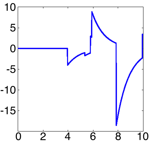
(a) Poisson, $\lambda=0.5$

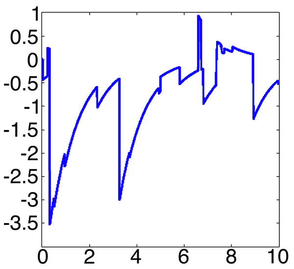
(b) Poisson, $\lambda=3$

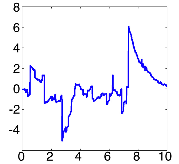
(c) Poisson, $\lambda=100$

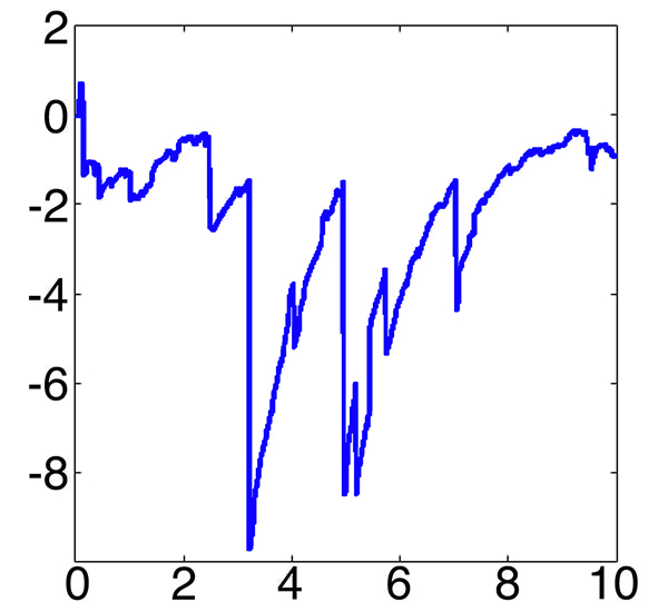
(d) Cauchy, $\lambda\rightarrow\infty$

Figure 3: Processes generated by $\mathrm{D}+\alpha\mathrm{I}$, $\alpha=0.1$, so that $s=(\mathrm{D}+\alpha\mathrm{I})^{-1}w$. In (a)-(c), $w$ is a Poisson noise with Cauchy jumps, with increasing $\lambda$. In (d), $w$ is a Cauchy white noise.

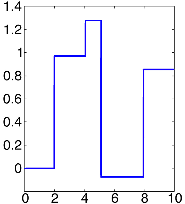
(a) Poisson, $\lambda=0.5$

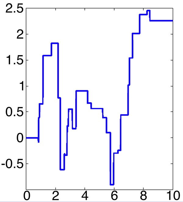
(b) Poisson, $\lambda=3$

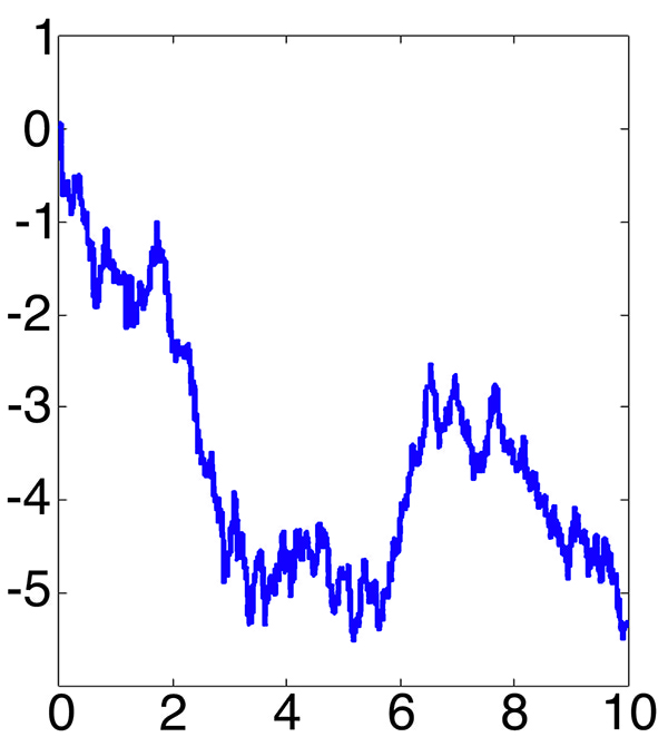
(c) Poisson, $\lambda=100$

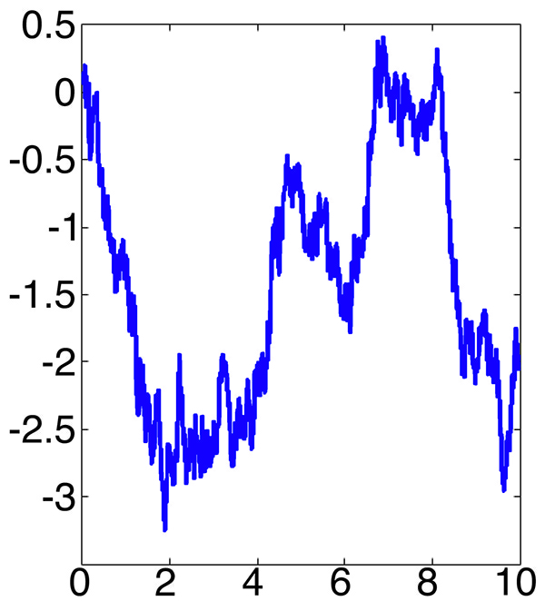
(d) Gaussian, $\lambda\rightarrow\infty$

Figure 4: Processes whitened by $\mathrm{D}$. In (a)-(c), $w$ is a Poisson noise with Gaussian jumps, with increasing $\lambda$. In (d), $w$ is a Gaussian white noise.

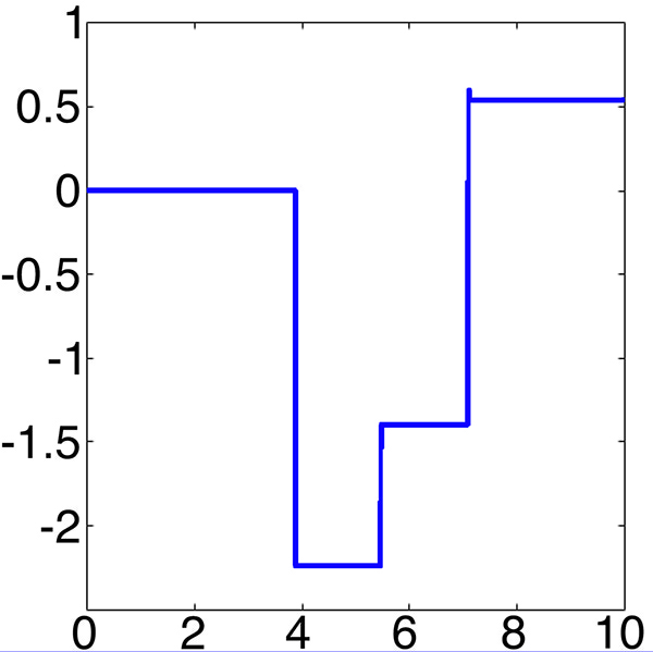
(a) Poisson, $\lambda=0.5$

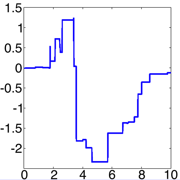
(b) Poisson, $\lambda=3$

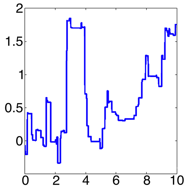
(c) Poisson, $\lambda=100$

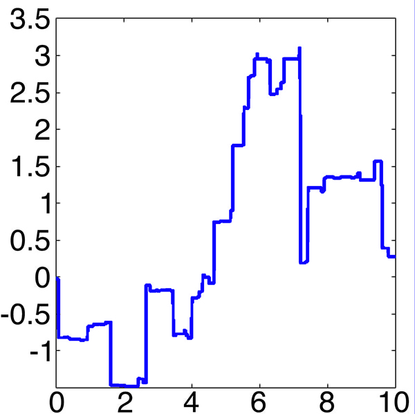
(d) Laplace, $\lambda\rightarrow\infty$

Figure 5: Processes generated by $\mathrm{D}$, so that $s=\mathrm{D}^{-1}w$. In (a)-(c), $w$ is a Poisson noise with Laplace jumps, with increasing $\lambda$. In (d), $w$ is a Laplace white noise.

VI-B Simulations in 2-D

We illustrate three families of 2-D processes $s$, given as

• $\mathrm{D}_{x}\mathrm{D}_{y}s=w$;

• $(\mathrm{D}_{x}+\alpha\mathrm{I})(\mathrm{D}_{y}+\alpha\mathrm{I})s=w$, with parameter $\alpha>0$;

• $(-\Delta)^{\gamma/2}s=w$, with parameter $\gamma>0$.

We represent our 2-D examples in two ways: first as an image, with gray levels that correspond to the amplitude of the process (lowest value is dark, highest value is white); second as a 3-D plot. All processes are plotted on $[0,10]^{2}$. In Figures 6 and 7, we show a Gaussian process with $D$ as whitening operator. A Gaussian process generated by the fractional Laplacian $(-\Delta)^{\frac{\gamma}{2}}$ is illustrated in Figures 8 and 9. Finally, we plot in Figures 10 and 11 a Laplace process generated by $\mathrm{D}+\alpha\mathrm{I}$. We always first show the process generated with an appropriate Poisson noise with increasing $\lambda$ and then plot the processes obtained from the corresponding Lévy white noise.

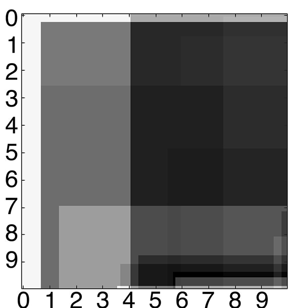
(a) Poisson, $\lambda=0.1$

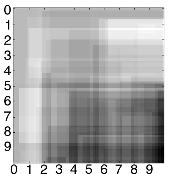
(b) Poisson, $\lambda=1$

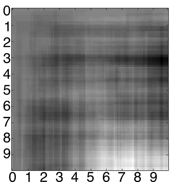
(c) Poisson, $\lambda=50$

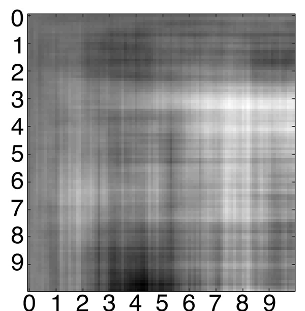
(d) Gaussian, $\lambda\rightarrow\infty$

Figure 6: Processes generated by $\mathrm{D}$, so that $s=\mathrm{D}^{-1}w$. In (a)-(c), $w$ is a Poisson noise with Gaussian jumps, with increasing $\lambda$. In (d), $w$ is a Gaussian white noise.

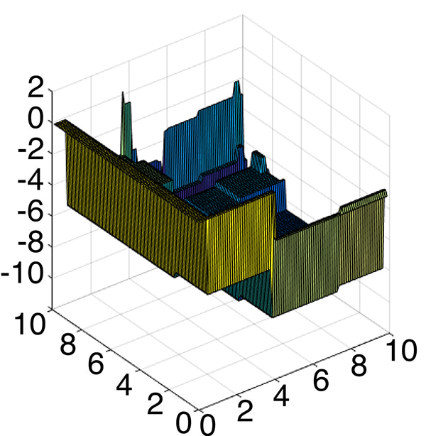
(a) Poisson, $\lambda=0.1$

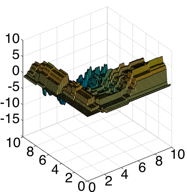
(b) Poisson, $\lambda=1$

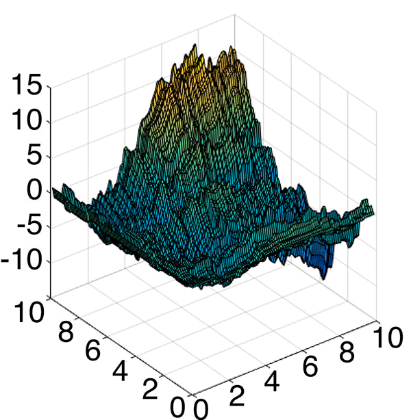
(c) Poisson, $\lambda=50$

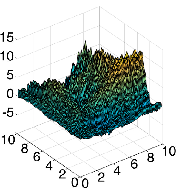
(d) Gaussian, $\lambda\rightarrow\infty$

Figure 7: 3-D representation of processes generated by $\mathrm{D}$, so that $s=\mathrm{D}^{-1}w$. In (a)-(c), $w$ is a Poisson noise with Gaussian jumps, with increasing $\lambda$. In (d), $w$ is a Gaussian white noise.

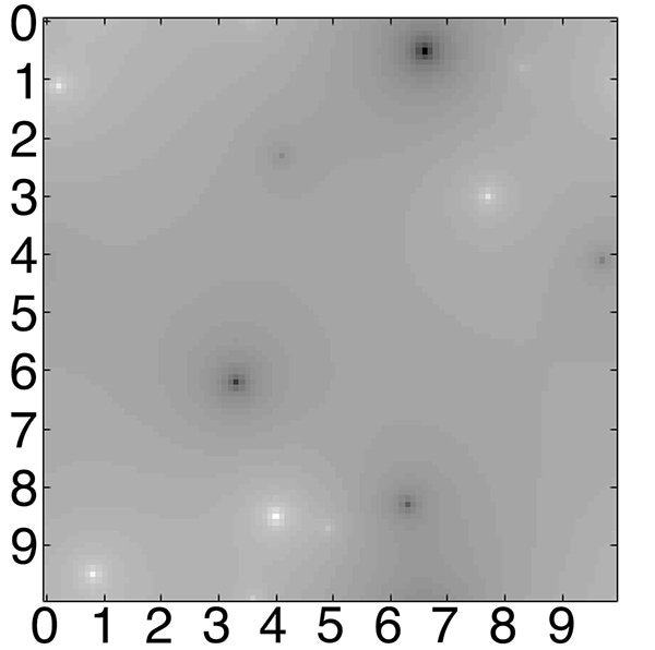
(a) Poisson, $\lambda=0.1$

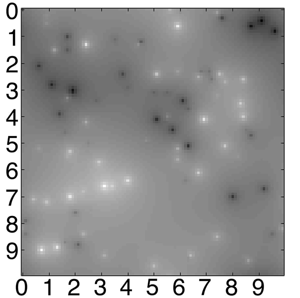
(b) Poisson, $\lambda=1$

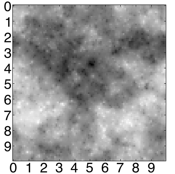
(c) Poisson, $\lambda=50$

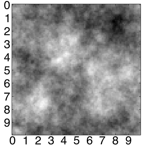
(d) Gaussian, $\lambda\rightarrow\infty$

Figure 8: Processes generated by $(-\Delta)^{\frac{\gamma}{2}}$, $\gamma=1.5$, so that $s=((-\Delta)^{\frac{\gamma}{2}})^{-1}w$. In (a)-(c), $w$ is a Poisson noise with Gaussian jumps, with increasing $\lambda$. In (d), $w$ is a Gaussian white noise.

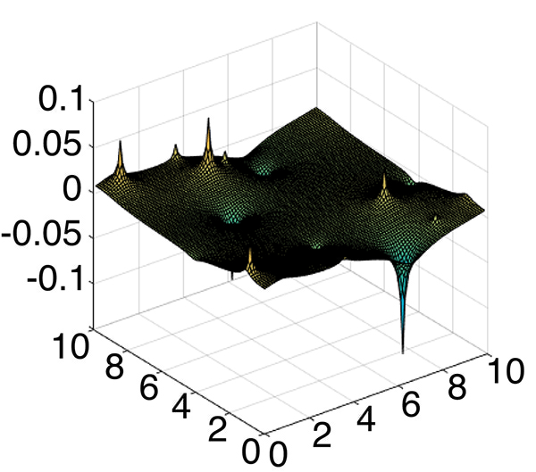
(a) Poisson, $\lambda=0.1$

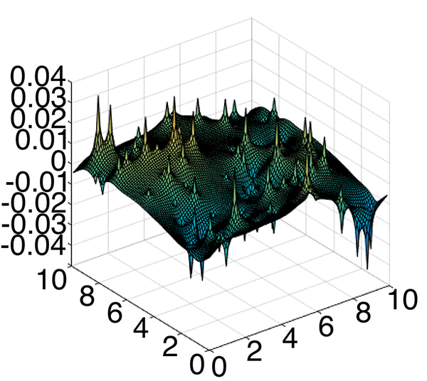
(b) Poisson, $\lambda=1$

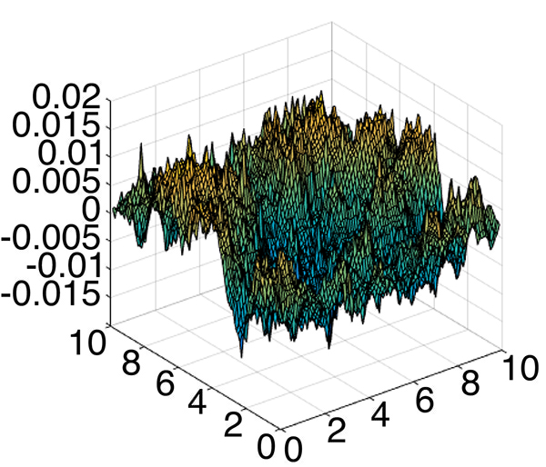
(c) Poisson, $\lambda=50$

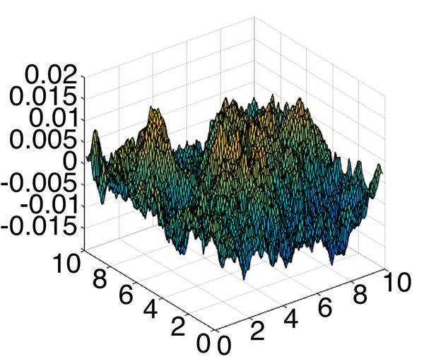
(d) Gaussian, $\lambda\rightarrow\infty$

Figure 9: 3-D representation of processes generated by $(-\Delta)^{\frac{\gamma}{2}}$, $\gamma=1.5$, so that $s=((-\Delta)^{\frac{\gamma}{2}})^{-1}w$. In (a)-(c), $w$ is a Poisson noise with Gaussian jumps, with increasing $\lambda$. In (d), $w$ is a Gaussian white noise.

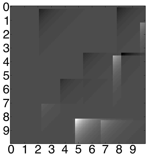
(a) Poisson, $\lambda=0.1$

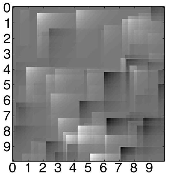
(b) Poisson, $\lambda=1$

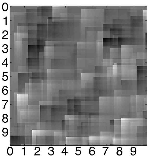
(c) Poisson, $\lambda=50$

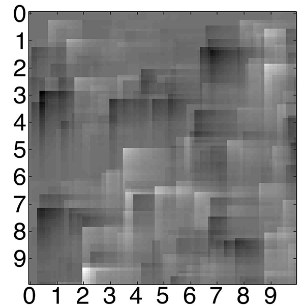
(d) Laplace, $\lambda\rightarrow\infty$

Figure 10: Processes generated by $(\mathrm{D}_{x}+\alpha\mathrm{I})(\mathrm{D}_{y}+\alpha\mathrm{I})$, $\alpha=0.1$, so that $s=\left((\mathrm{D}_{x}+\alpha\mathrm{I})(\mathrm{D}_{y}+\alpha\mathrm{I})\right)^{-1}w$. In (a)-(c), $w$ is a Poisson noise with Laplace jumps, with increasing $\lambda$. In (d), $w$ is a Laplace white noise.

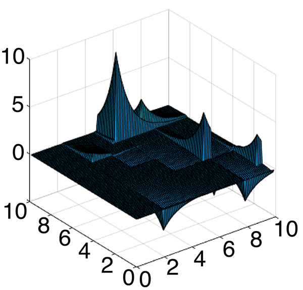
(a) Poisson, $\lambda=0.1$

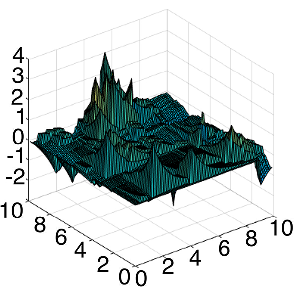
(b) Poisson, $\lambda=1$

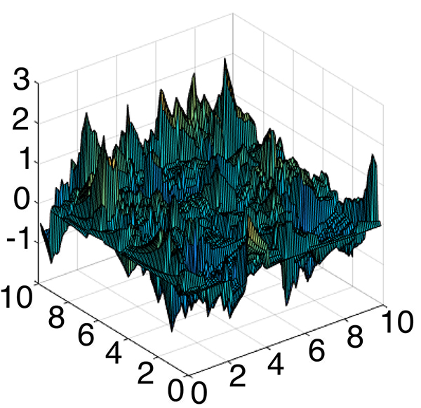
(c) Poisson, $\lambda=50$

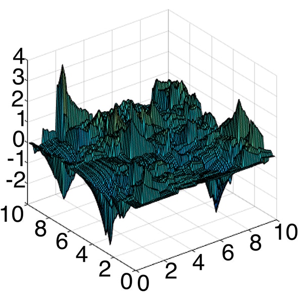
(d) Laplace, $\lambda\rightarrow\infty$

Figure 11: 3-D representation of processes generated by $(\mathrm{D}_{x}+\alpha\mathrm{I})(\mathrm{D}_{y}+\alpha\mathrm{I})$, $\alpha=0.1$, so that $s=\left((\mathrm{D}_{x}+\alpha\mathrm{I})(\mathrm{D}_{y}+\alpha\mathrm{I})\right)^{-1}w$. In (a)-(c), $w$ is a Poisson noise with Laplace jumps, with increasing $\lambda$. In (d), $w$ is a Laplace white noise.

VII Conclusion

Our main result in this work is the proof that any generalized Lévy process $s=\mathrm{L}^{-1}w$ is the limit in law of generalized Poisson processes obeying the same equation, but where $w$ corresponds to an appropriate impulsive Poisson noises. In addition, we showed that generalized Poisson processes are random $\mathrm{L}$-splines. In the asymptotic regime, generalized Lévy processes can thus conveniently be described using splines.

This result is interesting in practice as it provides a new way of efficiently generating approximations of broad classes of sparse processes $s=\mathrm{L}^{-1}w$. The only remaining requirement is the ability to generate the infinitely divisible random variable that drives the white noise $w$. From Theorem 1, the resulting approximation is guaranteed to be statistically identical to the original $s$. This confirms the remarkable intuition that Bode and Shannon enunciated decades before the formulation of the mathematical tools needed to prove their claims.

References

- [1] H. W. Bode and C. E. Shannon, “A simplified derivation of linear least square smoothing and prediction theory,” Proceedings of the IRE, vol. 38, no. 4, pp. 417–425, 1950.
- [2] M. Unser, “Splines: A perfect fit for signal and image processing,” IEEE Signal Processing Magazine, vol. 16, no. 6, pp. 22–38, 1999.
- [3] I. Schoenberg, Cardinal Spline Interpolation. SIAM, 1973, vol. 12.
- [4] M. Schultz and R. Varga, “L-splines,” Numerische Mathematik, vol. 10, no. 4, pp. 345–369, 1967.
- [5] W. Madych and S. Nelson, “Polyharmonic cardinal splines,” Journal of Approximation Theory, vol. 60, no. 2, pp. 141–156, 1990.
- [6] M. Unser and T. Blu, “Fractional splines and wavelets,” SIAM Review, vol. 42, no. 1, pp. 43–67, 2000.
- [7] M. Unser and P. D. Tafti, “Stochastic models for sparse and piecewise-smooth signals,” IEEE Transactions on Signal Processing, vol. 59, no. 3, pp. 989–1006, 2011.
- [8] M. Vetterli, J. Kovačević, and V. K. Goyal, Foundations of Signal Processing. Cambridge University Press, 2014.
- [9] M. Unser and P. D. Tafti, An Introduction to Sparse Stochastic Processes. Cambridge University Press, 2014.
- [10] B. Mandelbrot and J. V. Ness, “Fractional Brownian motions, fractional noises and applications,” SIAM Review, vol. 10, no. 4, pp. 422–437, 1968.
- [11] B. Mandelbrot, The Fractal Geometry of Nature. W. H. Freeman and Co., San Francisco, California, 1982.
- [12] B. Pesquet-Popescu and J. L. Véhel, “Stochastic fractal models for image processing,” IEEE Signal Processing Magazine, vol. 19, no. 5, pp. 48–62, 2002.
- [13] T. Blu and M. Unser, “Self-similarity: Part II—Optimal estimation of fractal processes,” IEEE Transactions on Signal Processing, vol. 55, no. 4, pp. 1364–1378, 2007.
- [14] D. Mumford and B. Gidas, “Stochastic models for generic images,” Quarterly of Applied Mathematics, vol. 59, no. 1, pp. 85–112, 2001.
- [15] D. Mumford and A. Desolneux, Pattern Theory: The Stochastic Analysis of Real-World Signals. A.K. Peters, Ltd., Natick, MA, 2010.
- [16] A. Srivastava, A. Lee, E. Simoncelli, and S.-C. Zhu, “On advances in statistical modeling of natural images,” Journal of Mathematical Imaging and Vision, vol. 18, no. 1, pp. 17–33, 2003.
- [17] C. Nikias and M. Shao, Signal Processing with Alpha-Stable Distributions and Applications. Wiley-Interscience, 1995.
- [18] K. Sato, Lévy Processes and Infinitely Divisible Distributions. Cambridge University Press, 2013, vol. 68.
- [19] L. Schwartz, Théorie des distributions. Hermann, 1966.
- [20] K. Itō, “Stationary random distributions,” Kyoto Journal of Mathematics, vol. 28, no. 3, pp. 209–223, 1954.
- [21] I. Gelfand, “Generalized random processes,” Doklady Akademii Nauk SSSR, vol. 100, pp. 853–856, 1955.
- [22] I. Gelfand and N. Vilenkin, Generalized Functions. Vol. 4: Applications of Harmonic Analysis. Academic Press, New York-London, 1964.
- [23] K. Itō, Foundations of Stochastic Differential Equations in Infinite Dimensional Spaces. SIAM, 1984, vol. 47.
- [24] E. Perrin, R. Harba, C. Berzin-Joseph, I. Iribarren, and A. Bonami, “Nth-order fractional Brownian motion and fractional Gaussian noises,” IEEE Transactions on Signal Processing, vol. 49, no. 5, pp. 1049–1059, 2001.
- [25] P. D. Tafti and M. Unser, “Fractional Brownian vector fields,” Multiscale Modeling & Simulation, vol. 8, no. 5, pp. 1645–1670, 2010.
- [26] A. Lodhia, S. Sheffield, X. Sun, and S. Watson, “Fractional gaussian fields: A survey,” Probability Surveys, vol. 13, pp. 1–56, 2016.
- [27] H. Biermé, A. Estrade, and I. Kaj, “Self-similar random fields and rescaled random balls models,” Journal of Theoretical Probability, vol. 23, no. 4, pp. 1110–1141, 2010.
- [28] J. Fageot, E. Bostan, and M. Unser, “Wavelet statistics of sparse and self-similar images,” SIAM Journal on Imaging Sciences, vol. 8, no. 4, pp. 2951–2975, 2015.
- [29] G. Samorodnitsky and M. Taqqu, Stable Non-Gaussian Processes: Stochastic Models with Infinite Variance. Chapman and Hall, 1994.
- [30] S. Koltz, T. Kozubowski, and K. Podgorski, The Laplace Distribution and Generalizations. Boston, MA: Birkhauser, 2001.
- [31] B. Grigelionis, Student’s T-Distribution and Related Stochastic Processes. Springer, 2013.
- [32] D. Applebaum, Lévy Processes and Stochastic Calculus. Cambridge University Press, 2009.
- [33] P. Brockwell and J. Hannig, “CARMA (p,q) generalized random processes,” Journal of Statistical Planning and Inference, vol. 140, no. 12, pp. 3613–3618, 2010.
- [34] P. Brockwell, “Lévy-driven CARMA processes,” Annals of the Institute of Statistical Mathematics, vol. 53, no. 1, pp. 113–124, 2001.
- [35] A. Durand and S. Jaffard, “Multifractal analysis of Lévy fields,” Probability Theory and Related Fields, vol. 153, no. 1-2, pp. 45–96, 2012.
- [36] M. Vetterli, P. Marziliano, and T. Blu, “Sampling signals with finite rate of innovation,” IEEE Transactions on Signal Processing, vol. 50, no. 6, pp. 1417–1428, 2002.
- [37] J. Fageot, J. Ward, and M. Unser, “Interpretation of continuous-time autoregressive processes as random exponential splines,” in Proceedings of the Eleventh International Workshop on Sampling Theory and Applications (SampTA’15), Washington DC, USA, May 25-29, 2015, pp. 231–235.
- [38] M. Unser and T. Blu, “Cardinal exponential splines: Part I—Theory and filtering algorithms,” IEEE Transactions on Signal Processing, vol. 53, no. 4, pp. 1425–1438, 2005.
- [39] ——, “Self-similarity: Part I—Splines and operators,” IEEE Transactions on Signal Processing, vol. 55, no. 4, pp. 1352–1363, 2007.
- [40] D. Van De Ville, T. Blu, and M. Unser, “Isotropic polyharmonic B-splines: Scaling functions and wavelets,” IEEE Transactions on Image Processing, vol. 14, no. 11, pp. 1798–1813, 2005.
- [41] A. Pietsch, Nuclear Locally Convex Spaces. Springer, 1972.
- [42] F. Trèves, Topological Vector Spaces, Distributions and Kernels. Academic Press, New York-London, 1967.
- [43] A. Grothendieck, Produits tensoriels topologiques et espaces nucléaires. American Mathematical Society, 1955, no. 16.
- [44] D. Mushtari, Probabilities and Topologies on Linear Spaces. Kazan Mathematics Foundation, 1996, vol. 1.
- [45] R. Minlos, “Generalized random processes and their extension in measure,” Trudy Moskovskogo Matematicheskogo Obshchestva, vol. 8, pp. 497–518, 1959.
- [46] X. Fernique, “Processus linéaires, processus généralisés,” Annales de l’Institut Fourier, vol. 17, pp. 1–92, 1967.
- [47] P. Boulicaut, “Convergence cylindrique et convergence étroite d’une suite de probabilités de Radon,” Zeitschrift für Wahrscheinlichkeitstheorie und verwandte Gebiete, vol. 28, no. 1, pp. 43–52, 1973/74.
- [48] J. Fageot, A. Amini, and M. Unser, “On the continuity of characteristic functionals and sparse stochastic modeling,” Journal of Fourier Analysis and Applications, vol. 20, no. 6, pp. 1179–1211, 2014.
- [49] M. Unser, P. D. Tafti, and Q. Sun, “A unified formulation of Gaussian versus sparse stochastic processes—Part I: Continuous-domain theory,” IEEE Transactions on Information Theory, vol. 60, no. 3, pp. 1945–1962, 2014.
- [50] R. Horn, “Quadratic forms in harmonic analysis and the Bochner-Eberlein theorem,” Proceedings of the American Mathematical Society, vol. 52, no. 1, pp. 263–270, 1975.