Fractal scaling of turbulent premixed flame fronts: application to LES

Abstract

The fractal scaling properties of turbulent premixed flame fronts have been investigated and considered for modelling sub-grid scales in the Large-Eddy-Simulation framework. Since the width of such thin reaction fronts cannot be resolved into the coarse mesh of LES, the extent of wrinkled flame surface contained in a volume is taken into account. The amount of unresolved flame front is estimated via the “wrinkling factor” that depends on the definition of a suitable fractal dimension and the scale at which the fractal scaling is lost, the inner cut-off length $\epsilon_{i}$. In this context, the present study considers laboratory experiments and one-step reaction DNS of turbulent premixed jet flames in different regimes of turbulent premixed flames. Fractal dimension is found to be substantially constant and well below that typical of passive scalar fronts. The inner cut-off length shows a clear scaling with the dissipative scale of Kolmogorov for the regimes here considered. These features have been exploited performing Large Eddy Simulations. Good model performance has been found comparing the LES against a corresponding DNS at moderate Reynolds number and experimental data at higher Reynolds numbers.

1 Introduction

Turbulent premixed combustion at high Reynolds numbers is characterized by the interplay of hydrodynamic flow field, heat release and pressure waves, see e.g. [1, 2]. This intrinsic coupling leads to a substantial large scale unsteadiness that can be captured by the time resolving feature of Large Eddy Simulation (LES), making this approach extremely appealing. LES computes explicitly the time dependent dynamics of the large-scale structures of the flow, modelling the effects of the unresolved small scales, the so-called sub-grid scales. In premixed combustion, the success of the approach crucially depends on the ability of modelling the interaction between chemistry and turbulence, which occurs in thin reaction regions below the resolved scales.

Several different approaches are described in literature. A possible methodology consists in artificially thickening the reaction zone, to make it resolved on the computational mesh. Such artificial thickening modifies the interaction between turbulence and chemistry and requires the introduction of a suitable efficiency function involving several empirical parameters to recover the correct behaviour, [3, 4]. Alternatively, the propagative nature of the flame front can be exploited in the context of so-called G-equation methods, where the flame front is represented by a particular iso-surface of a continuous scalar field $G$ moving with the given speed of the front, [5, 6, 7, 8, 9].

Sticking to classical sub-grid formulations for turbulent stresses and transport, the specific combustion closure we pursue in this work is inspired to the multiscale nature of turbulent flame fronts, [10, 11]. When the area of an instantaneous flame front surface is measured at increasingly finer resolutions, the measure increases, following a power law with exponent $D$. The exponent is typically non-integer, smaller than the dimension of the embedding space ($D_{E}=3$) and larger than the topological dimension of a smooth surface ($D_{T}=2$), thus characterising the front as a fractal, [12]. In fact, the area increase follows the fractal power law until an inner cut-off is eventually reached. For finer resolutions the scaling is lost and the smooth behaviour is recovered. In the technical literature this kind of objects are called pre-fractals, [13].

In the context of fractal approaches for premixed combustion modelling, a simple choice consists in describing the reactions in terms of a single progress variable $c$, determined either from temperature $T$ or fuel mass-fraction $Y_{R}$, e.g. $c=(T-T_{u})/(T_{b}-T_{u})$, with the subscripts $b$ and $u$ denoting burned and unburned states, respectively. The progress variable evolves according to an advection/diffusion/reaction equation, where the reaction term $\dot{\omega}$ is often given by a global Arrenhius law. Similarly to G-equation methods, the propagative nature of the front can be exploited to recast the diffusion and reaction terms into a single propagative contribution characterised by a suitable phase speed, $S_{L}$, corresponding to the unstrained Laminar flame speed, [14],

$${\bf\nabla}\cdot{(\rho D\nabla c)}+{\dot{\omega}}=\rho_{u}S_{L}|\nabla{c}|~{}\ .$$ (1)

Here $\rho$ is the density, $\dot{\omega}$ the reaction rate and $D$ the molecular diffusivity. In this framework, LES involves the convolution of the RHS of eq. (1) with a filter of width $\Delta$. The result is expressed in terms of flame surface density $\Sigma=\overline{|\nabla c}|$, with the overline denoting filtering. $\Sigma$ represents the convoluted front area contained in a volume of dimension $\Delta$. A number of closures for $\Sigma$ has been proposed in literature, starting with simple algebraic expressions originally introduced by [15]. More directly related to our present interest is the link with the fractal properties of the front, [11]. In this case, the model exploits the self-similar fractal nature of progress variable isosurfaces that are wrinkled and folded by turbulence over a wide range of scales, from the integral length scale down to an inner cut-off $\epsilon_{i}<\Delta$. The wrinkling factor $\Xi=\overline{|\nabla c}|/|\nabla\overline{c}|$ relates the flame surface density to the gradient of the filtered progress variable $\overline{c}$ and corresponds to the ratio of the two areas measured at scales $\Delta$ ($A(\Delta)$) and $\epsilon_{i}$ ($A(\epsilon_{i})$), respectively.

As already mentioned, the measure of the front surface scales with a power law whose exponent, namely the fractal dimension $D$, is known to be constant down to $\epsilon_{i}$. More in details, the filtered progress variable equation reads

$$\frac{\partial\overline{\rho}\tilde{c}}{\partial t} +{\bf\nabla}\cdot(\overline{\rho}\tilde{\bf{u}}\tilde{c})+{\bf\nabla}\cdot{(\overline{\rho}\widetilde{{\bf{u}}c}-\overline{\rho}\tilde{\bf{u}}\tilde{c})}={\bf\nabla}\cdot\overline{(\rho D\nabla c)}+\overline{\dot{\omega}}=\rho_{u}S_{L}\Xi|\nabla\tilde{c}|~{},$$ (2)

where $\overline{\cdot}$ and $\tilde{\cdot}$ denote Reynolds and Favre averaging, respectively, and $\bf{u}$ is the velocity. Following [11, 16], the model can be closed using the fractal behaviour of flames

$$\Xi({\Delta})\propto(\Delta/\epsilon_{i})^{D-2}\ .$$ (3)

After properly identifying the inner cut-off $\epsilon_{i}$, this approach circumvents the problem found in LES where reactive processes act in the unresolved range of scales, below the LES filter width.

Coming back to our purposes, a crucial issue of this fractal model is the determination of the fractal dimension $D$ and of the inner cut-off $\epsilon_{i}$ and their dependence on turbulence/chemistry conditions.

Some studies investigated the fractal features of premixed flames, i.e. the fractal dimension, the inner and the outer cut-offs, see for example [17, 18]. The main aim is to determine the dependence of these parameters on turbulence, thermodynamics and flame features.
Pioneering investigations on the fractal features of interfaces passively transported in non reactive turbulent flows as wakes beyond bodies, jet flows or mixing layers can be found in [19, 20]. The experimental findings indicating a fractal dimension of 2.37 and a cut-off length proportional to the Kolmogorov dissipative length was also supported by an interesting theoretical reasoning based on the Kolmogorov K41 theory and intermittency corrections. However the mechanism producing a surface wrinkling in cold (incompressible) turbulent flows is deeply different from what happens to the flame front wrinkled by the turbulent structures where the thermal expansion due to the combustion induces additional phenomenologies. Actually, concerning turbulent premixed flames, the fractal dimension appears to show a wide variation between 2.18-2.35, see e.g. [21, 22], and the inner cut-off length dependence is still debated [23]. The outer cut-off scale is generally accepted to be grater than the turbulence integral scale [22], however it should be noted that this information is not needed in the LES framework. [24] reports a geometric interpretation on fractal flame features analysing data of a turbulent premixed Bunsen flame. They illustrate the relations between the inner and outer cut-off length with the turbulence and flame properties. The study in [22] presents an extensive experimental analysis of a premixed propane/air flame using OH-LIF and Mie-Scattering, with different turbulence intensities $u^{\prime}/S_{L}$ and Reynolds numbers. The paper discusses also the possible errors induced by experimental image acquisition technique showing a strong dependency on the employed methodology and providing technical explanation of observed differences. Furthermore the authors remark as the large discrepancy between predictions and previous studies calls for new investigations.
To partially overcome these difficulties a dynamic fractal model for LES has been developed by [11, 25] exploiting the self-similar nature of the process. The model was tested using a-priori analysis on experimental data concerning turbulent premixed propane/air flame stabilised with a triangular bluff body. Data show a good agreement between the a-priori model prediction and the experimental data.

Aim of the present work is twofold, on one hand the experimental and numerical evaluation of both the exponent $D$ and $\epsilon_{i}$ by OH-LIF –Laser Induced Fluorescence– on premixed methane/air jet flames in round and annular configurations. On the other hand, on the ground of the fractal characteristics found, we aim to accurately compare the Large-Eddy-Simulation data with a corresponding DNS of a turbulent premixed flame at moderately low Reynolds number, i.e. $Re=U_{b}D\rho/\mu=6000$ ($U_{b}$ is the bulk jet velocity and $D$ is the nozzle diameter) and to reproduce the main features of the higher Reynolds number experiments ($Re=16000$ and $Re=24000$) carried out by [26].

Results show that fractal exponent $D=2.23$, smaller than in non-reactive cases, appears to be rather insensitive to the explored Reynolds numbers, turbulence and flame features and to the configurations adopted. It follows that fractal dimension can be considered as a fixed parameter for turbulent combustion processes. The experimental analysis on the inner cut-off $\epsilon_{i}$ shows that it scales with the dissipative Kolmogorov length $\eta_{k}$ in the regimes here analysed. The results of the Large-Eddy-Simulations using these assumptions well agree with the corresponding reference data.

2 Fractal characteristics of flame fronts

The fractal features of the flame front of turbulent premixed flames are extracted analysing experimental and numerical (DNS) data. The dataset pertains to a wide range of flame regimes as can be appreciated in figure 1 where a turbulent flame classification diagram is reported with the present experiments (closed symbols) and DNS (open symbols).

2.1 Methodology

2.1.1 Experimental set-up

Methane/air premixed flames have been realised in two different jet-burners. The first is a cylindrical bunsen burner, whose inner diameter is $D=18$ mm. A diffusive methane pilot flame anchored the flame to the nozzle exit. Reynolds numbers (diameter based, i.e. $Re=U_{b}D/\nu$) and equivalence ratios ($\Phi$) ranges between $Re=7000$ and $Re=10000$ and from stoichiometric mixtures down to $\Phi=0.6$ [27]. The second is a stainless steel annular inlet bluff-body stabilised burner (nozzle outer diameter $D=25$ mm, inner diameter $D_{i}=15$ mm) fed with a mixture of $CH_{4}$ and air at different equivalence ratios. The Reynolds number evaluated by the bulk velocity and the nozzle diameter is kept fixed at a value of $Re=U_{b}D/\nu=10^{4}$, to ensure a fully developed turbulent jet with well-defined turbulence characteristics [28]. In this case the flame is anchored by the recirculation due to a conical bluff-body. Four different flames are investigated and their methane/air equivalence ratio $\Phi$ is varied in the range of $[0.6-1.12]$. Velocity data comes from LDA and PIV measurements by seeding the flow with $5~{}\mu$m alumina particles [29, 30]. The flame classification of the present experiments spans from the beginning of the thickened flame to the corrugated flame regimes, as reported in figure 1.

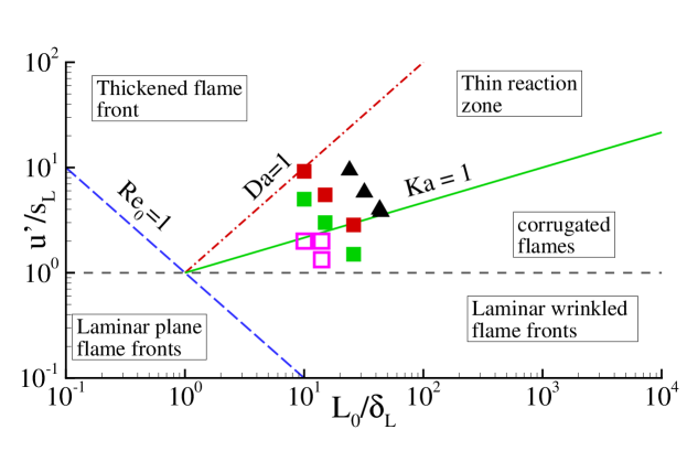
Figure 1: Right panel: Turbulent premixed flame classification diagram (Borghi) where present Experiments (closed symbols: squares round Bunsen jet at $Re=7000$ and $10000$, triangles annular jet at $Re=10000$) and DNS (open triangles $Re=4000$ and 6000) flame regimes are highlighted. In the figure, $u^{\prime}$ is the typical level of velocity fluctuations, $L_{0}$ the integral flow scale, $S_{L}$ and $\delta_{L}$ the laminar flame speed and thickness, respectively. $Ka=(\delta_{L}/\eta_{k})^{2}\sim(u^{\prime}/S_{L})^{3/2}\,(L_{0}/\delta_{L})^{-1/2}$ is the Karlovitz number ($\eta_{k}$ the Kolmogorov length) and $Da=S_{L}\,L_{0}/(u^{\prime}\,\delta_{L})$ is the Damköler number.

Flame front detection is performed instead by the acquisition of fluorescence signal emitted by OH radicals. To that end, a Nd:YAG laser beam is delivered through a tunable dye laser coupled with a second-harmonic generator crystal in order to shift the laser wavelength from $532$ nm down to $282.93$ nm, corresponding to the $Q_{1}(6)$ absorption line of OH. A suitable cylindrical lens expands the beam into a $350~{}\mu\rm{m}$ thick laser sheet. The resulting OH fluorescence emission is around $309$ nm and is then collected by a $1024\times 1024$ pixels ICCD ($2\times 2$ pixel binning) equipped with a $78$ mm Nikon quartz lens, resulting in a map of $512\times 512$ equivalent pixels with a resolution of $160~{}\mu\rm{m}$ for each equivalent pixel. Furthermore, a narrow pass-band filter, $10$ nm wide and centered at $310$ nm, isolates the relevant spectral line.

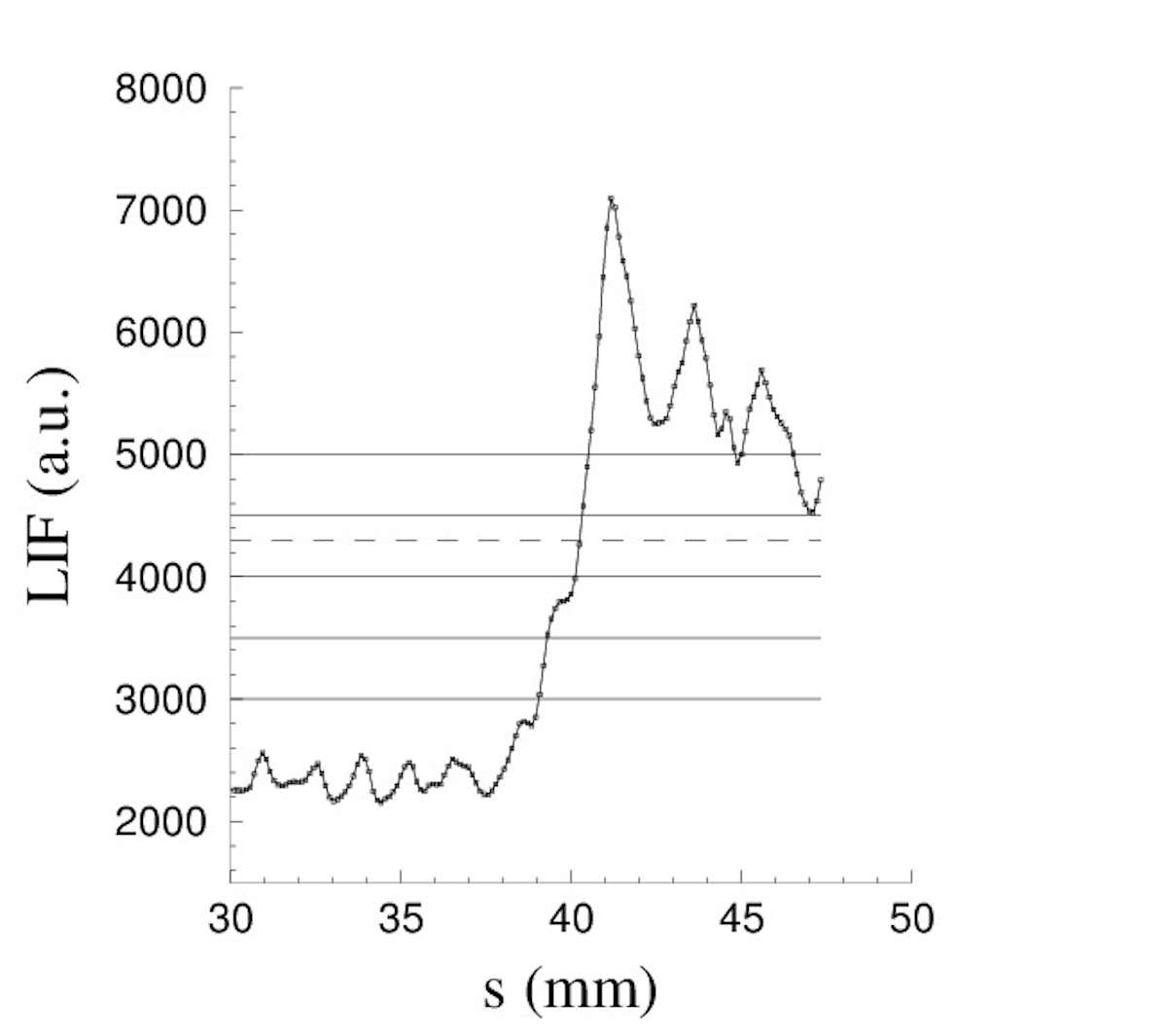
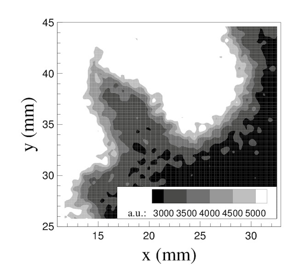
Figure 2: Left: OH fluorescence signal, $\Phi=1.03$. Dashed line corresponds to maximum gradient position. Abscissa $s$ originates at a point arbitrarily chosen in the reactants and crosses the flame front normally towards combustion products. Right: OH fluorescence map, $\Phi=1.03$. Gray levels refer to different OH threshold values, as reported in the legend.

The fluorescence signal from OH radical is proportional to its concentration and relative measurements are possible (absolute measurements of concentrations are instead prevented from non-radiative disexcitation channels that are generally active together with detectable fluorescence emission). An example of the LIF images taken with the experimental set-up described above is given in the right panel of figure 2. Here, the image portrays a detail of the whole flame and the signal level is reported in terms of CCD counts whose gray-color scale is shown in the inset appearing at the bottom. Moving from the zones in white color representative of higher level of fluorescence towards darker regions, it appears that the fluorescence signal decreases abruptly across the flame front, where the OH radicals are formed. This typical behaviour is shown in the left panel of figure 2 where a cut perpendicular to the flame front has been extracted from the image. Given that, within the products OH radicals disappear at a much slower rate than that characterising their formation in the flame, the consequent asymmetric behaviour can be used to distinguish between reactant and product zones. Based on this result, it is worth emphasising that even though in our measurements the signal-to-noise ratio is usually sufficiently large the gradient field may suffer from significant high-frequency contamination. All the same, the signal may be treated by suitable filtering techniques, e.g., the non linear filter described in [31], which provides satisfactory results in this case. Nonetheless, a variant of the threshold method [32] is adopted, which locates the front at the isoline that better correlates with the maximum gradient in the region of interest.

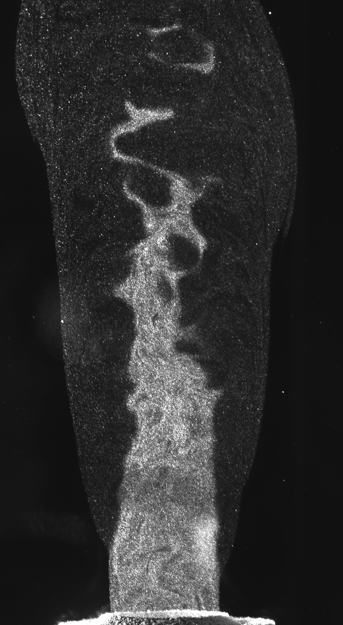
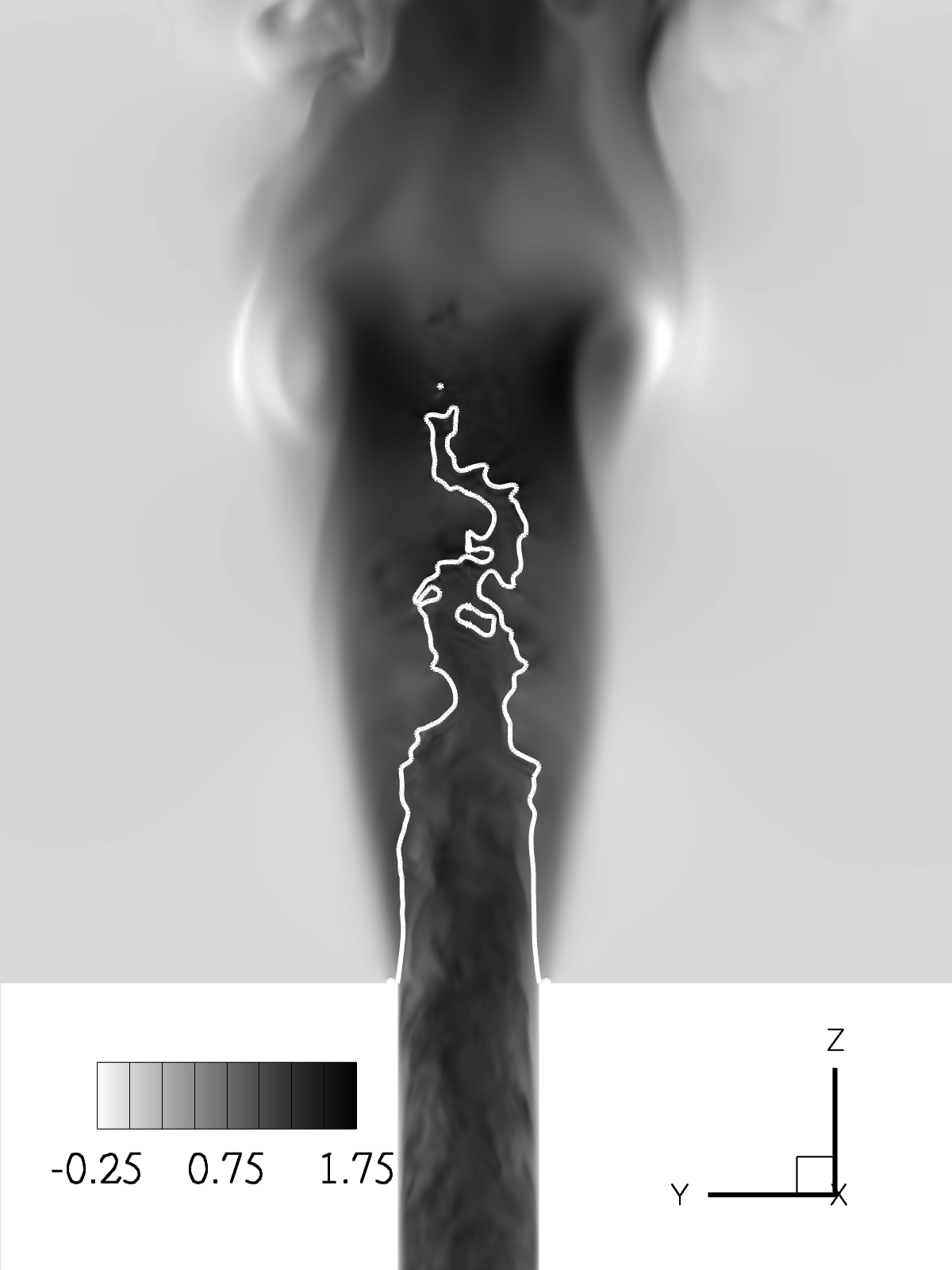
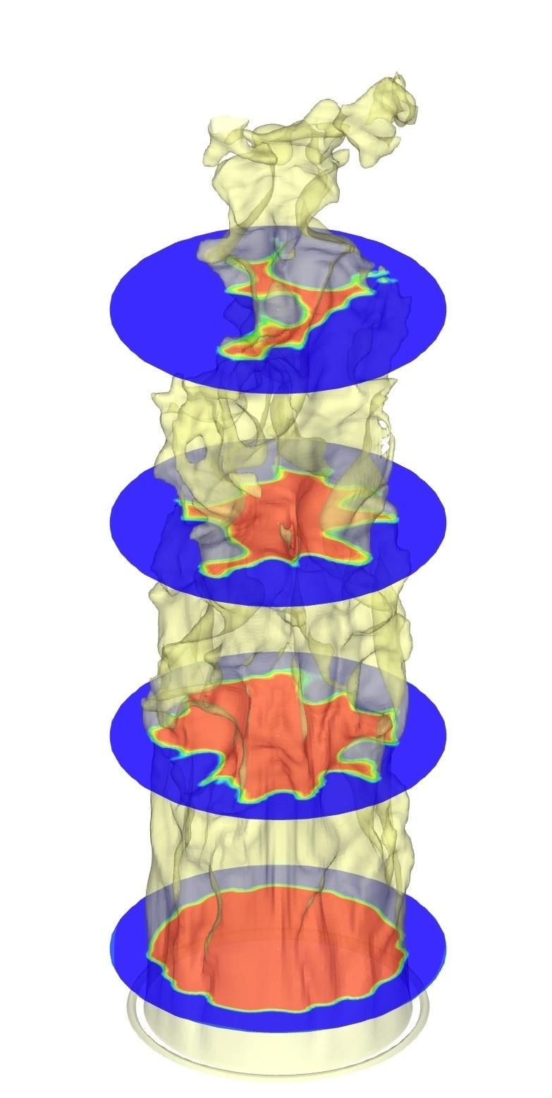
Figure 3: Snapshots. Left panel, raw mie scattering of the Bunsen flame at $Re=6000$; middle panel, DNS of a Bunsen flame at $Re=6000$: contours of axial velocity with superimposed a isolevel of $c=0.5$ in white; right panel, instantaneous 3D flame front detected by means of the reactant based progress variable isolevel $c=0.5$, four planes are superimposed to highlight the flame wrinkling.

2.1.2 Numerical Algorithm

The direct numerical simulation algorithm discretises the cylindrical formulation of the Low-Mach number asymptotic non-dimensional Navier-Stokes equations [33],

$$\frac{\partial\rho}{\partial t}+\nabla\cdot(\rho{\bf u})=0$$ (4)

$$\frac{\partial\rho\bf u}{\partial t}+\nabla\cdot({\rho\bf u\otimes\bf u})=\frac{1}{Re}\nabla\cdot{\bf\Sigma}-\nabla P+\rho{\bf g}$$ (5)

$$\frac{\partial\rho c}{\partial t}+\nabla\cdot({\rho{\bf u}c})=\frac{1}{ReSc}\nabla\cdot(\rho{\cal D}\nabla c)+\,\dot{\omega}$$ (6)

$$\nabla\cdot{\bf u}=\frac{1}{p}\left[\frac{1}{RePr}\nabla\cdot(k\nabla T)+\frac{\gamma-1}{\gamma}Ce\,\dot{\omega}\right]$$ (7)

$$T=\frac{p}{\rho}$$ (8)

where ${\bf\Sigma}=2\,\mu\,{\bf S}=\mu\,(\nabla\bf u+{\nabla\bf u}^{T})$ is the viscous stress tensor and $\mu$ is the viscosity dependence on temperature, $\rho$, $\bf u$ and $P$ are the density, the velocity and the dynamic pressure, respectively; $T$, $p$, $c=1-Y_{R}/Y_{R0}$ and $\dot{\omega}$ are the temperature, the thermodynamic pressure (constant in both space and time), the progress variable defined in terms of the local $Y_{R}$ and the inlet $Y_{R0}$ reactants concentration, and the corresponding reaction rate, respectively. ${\cal D}$ and $k$ are the progress variable diffusivity and the thermal conductivity, respectively. $Re=U_{b}D\rho_{0}/\mu_{0}$ is the Reynolds number, with $U_{b}$ the inlet bulk velocity, $D$ the nozzle diameter, and the subscript $0$ indicating the reference quantities corresponding to jet inlet conditions, $Pr=\mu_{0}/(k_{0}c_{p0})$ and $Sc=\mu_{0}/(\rho_{0}D_{0})$ are the Prandtl and the Schmidt numbers giving the ratio between thermal and mass diffusions on the viscosity $\mu_{0}$, respectively, here $c_{p0}$, $k_{0}$, and $D_{0}$ are the heat capacity at constant pressure, the thermal diffusivity and the mass diffusion evaluated at the reference state; $\gamma=c_{p}/c_{v}$ and $Ce=\rho_{0}\Delta H/p_{0}$ are the heat capacity coefficient ratio and the heat release parameter, respectively with $\Delta H$ the enthalpy of the reaction.

Spatial discretisation is obtained by central second order finite differences in conservative form on a staggered grid. The convective terms of scalar equations are discretised by a Bounded Central Difference Scheme to avoid spurious oscillations, see [34] for details. Temporal evolution is performed by a low-storage third order Runge-Kutta scheme.
Time-evolving boundary conditions are prescribed for the inflow where a fully turbulent inflow velocity is assigned at each time-step by using a cross-sectional slice of a fully developed pipe flow obtained by a companion DNS. In the middle panel of figure 3 the discharge of the fully turbulent pipe flow creating the jet is shown by contours of the fluctuating axial velocity. The density and the concentrations are kept fixed on the inflow nozzle. The outer part of the inlet region is constituted by an adiabatic wall. A convective Orlanski condition is adopted for outflow of all the variables, see also [35, 36, 37]. The artificial side boundary is modelled by an adiabatic traction-free condition to allow a correct entrainment rate. More details on the code and tests for incompressible jets can be found in [29, 37, 38, 39].

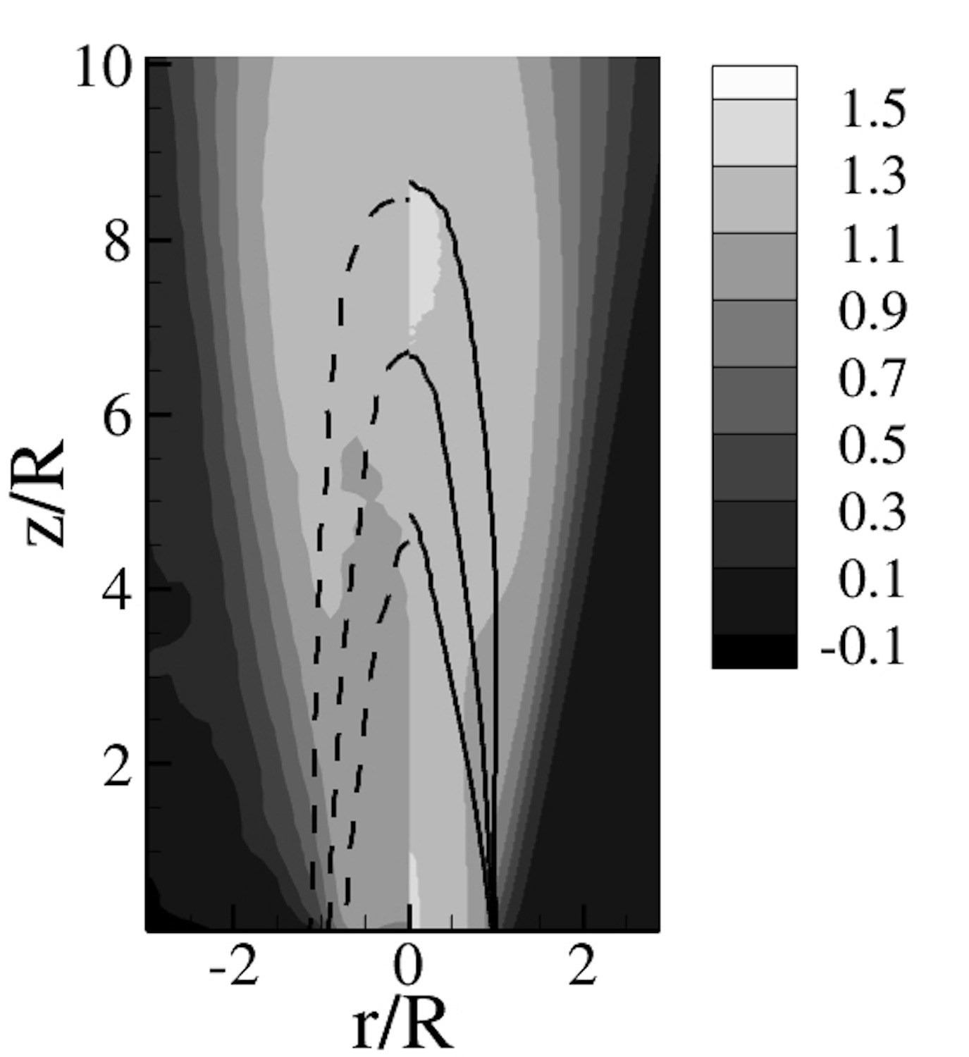
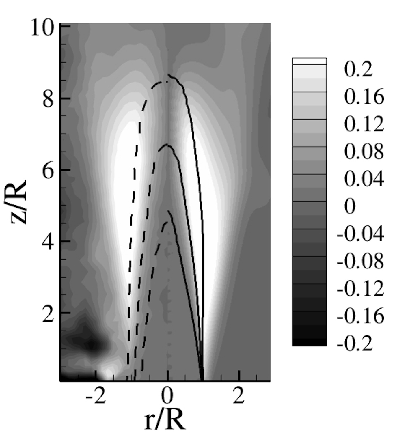
Figure 4: Mean flow field for experiments and DNS at $Re\simeq 6000$. Half-figures on the left represents experimental data, right half-figures the DNS ones. Right panel, axial mean velocity; left panel, radial mean velocity. The isolines provides three isolevels of the progress variable $c$: 0.25, 0.5, 0.75, namely.

Concerning the direct numerical simulation, the chemical kinetics is given by an Arrhenius single-step irreversible reaction which transforms the premixed fresh mixture $R$ into the exhaust gas of combustion products $P$: $\dot{\omega}=\omega^{0}(\rho Y_{R})e^{-T_{a}/T}$, with $\omega^{0}$ the reaction rate constant and $T_{a}$ the activation temperature.

Three DNS of premixed Bunsen jets are performed in order to reproduce the main features of premixed methane/air flames in conditions similar to the present experiments. The simulations replicate turbulent flames with $T_{f}/T_{0}\simeq 5.3$, and $S_{L}/U_{b}\simeq 0.05\div 0.075$ ($u^{\prime}\simeq 0.1\,U_{b}$) which can be classified according to the diagram shown in figure 1. As can be appreciated the DNSs are close to the straight line given by the Karlovitz number $Ka=1$ as usual in DNS simulations because of the constrained spatial resolution.

Concerning the input parameters assigned to the numerical code to simulate these flames, we have fixed $\gamma=1.3$ and $Ce=18.5$ in order to have a adiabatic flame temperature of $T_{f}=5.3\,T_{0}$  [40] ($T_{0}=300\,K$). The activation temperature is assumed $T_{a}\simeq 6\,T_{f}$, while the the reaction rate constant $\omega^{0}$ (made dimensionless by $U_{b}/R$) varies in the range $30000\div 67500$ together with the Reynolds number $Re=4000\div 6000$ in order to change $u^{\prime}/S_{L}$, i.e. $U_{b}/S_{L}$ and $L_{0}/\delta_{L}$ as reported in figure 1.

The flame has unitary Lewis number with $Pr=Sc=0.7$ while the diffusion coefficients depend on the temperature following the Sutherland-like law, $\mu/\mu_{0}=\rho{\cal D}/\rho_{0}{\cal D}_{0}=k/k_{0}=\,(T/T_{0})^{1/2}$.

The computational domain is given by: $[\theta_{max}\times R_{max}\times Z_{max}]=[2\pi\times 12.34\,R\times 14\,R]$ and it is discretised by $N_{\theta}\times N_{r}\times N_{z}=128\times 201\times 560$ points with stretched mesh in the radial direction to assure resolved shear layers with a radial grid spacing at the nozzle exit $\Delta R\simeq 1.5\eta_{k}$, with $\eta_{k}$ the pipe flow Kolmogorov length near the wall.
The general agreement between the instantaneous snapshots of the experimental and of the DNS flame in similar conditions ($Re=6000$, $\omega^{0}=45000$, $u^{\prime}/S_{L}\simeq 2$) is remarkable, see figure 3. A crucial issue for a correct reproduction of the experimental configuration is the accurate turbulent inflow conditions that avoid the use of synthetic turbulence or the mean advection of a frozen turbulent field. Actually, inlet conditions of the experiment and of the DNS are quite similar with the difference that a fully developed pipe is assigned to DNS, while in the experiments, inlet is generated by a pipe not long enough to provide fully developed statistics. Nonetheless, DNS with laminar inflows (not presented here) are characterised by the presence of large-scale motions influencing the whole reactive jet dynamics, whose behaviour is not observed experimentally. Figure 4 shows the mean flow behaviour for DNS and experiments in the same conditions, obtained by averaging about one-hundred instantaneous fields provided by DNS simulations and PIV-OH/LIF measurements. The general matching in terms of flame height and mean velocity is apparent.

2.2 Fractal scaling of the front

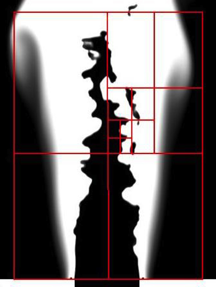
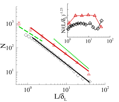
Figure 5: Left panel: Example of boxes of decreasing size used to cover the flame front. The image relates to the DNS data, but the same technique is applied to OH-LIF experimental data. Right panel: ensemble-averaged fractal scaling of 2D-cut flame front by means of box-counting. $N$ is the number of boxes at the respective measurement scale $L$. Abscissa has been made dimensionless by the laminar flame front thickness $\delta_{L}$. Symbols: Triangles, experiments on cylindrical Bunsen burner at $Re=7000$ $\Phi=1$; diamonds, DNS at $Re=6000$ and $u^{\prime}/S_{L}=2$. Thick lines are linear regressions of each ensemble-averaged data set in Log-scale ( $N\propto(L/\delta_{L})^{-1.23}$). Dash-dotted line is the theoretical fractal scaling for non-reacting scalar turbulent iso-surfaces, i.e. $N\propto(L/\delta_{L})^{-1.37}$. Long dashed line represents the viscous closure, $N\propto(L/\delta_{L})^{-1}$. Inset, compensated plot: $N/(L/\delta_{L})^{-1.23}$

The multiscale nature of the surface suggests the application of geometrical concepts from fractal theory to quantify the amount of flame wrinkling in terms of $\Xi$, see equation (3). In fractal theory, a power law relationship exists between the number of boxes needed to cover a fractal object and the box size $L$,

$$N(L)\propto L^{-D}~{},$$ (9)

where $D$ is defined as the fractal dimension of an object embedded in a three dimensional space. In our case, at least concerning the experiments, the fractal dimension $D_{2}$ is measured on two dimensional cuts of the flame front surface. Assuming isotropic properties of the flame front, the dimension of the whole 3D surface is expressed as: $D=D_{2}+1$. In real surfaces, the fractal scaling characterised by the dimension $D$ usually hold only in a limited range of scales between an inner ($\epsilon_{i}$) and an outer ($\epsilon_{o}$) cut-off lengths. Fractal characteristics of our experimental and numerical dataset have been evaluated by the box-counting technique, which consists in enumerating the squared boxes of size $L$ necessary to entirely cover the whole object that, in this case, is the flame front. If this number scales with equation (9), then the measured object is a fractal with dimension $D$ (or $D_{2}$ in 2D cuts). Right panel of figure 5 reports the fractal scaling of two flames, one measured and the other simulated. The plots show nice scalings maintained up to the inner cut-off length $\epsilon_{i}$, whose value has a direct impact on the wrinkling factor of equation (3); outer cut-offs are also apparent, though less important for LES applications. Data at different $u^{\prime}/S_{L}$ have been fitted with a power law whose exponents are reported in the left panel of figure 6. The fractal dimension $D$ shows an almost constant value of $D=2.23\pm 0.03$, well lower than $D=2.37$ which corresponds to perfectly passive scalar iso-surface fractal dimension as evaluated by [13]. It should be remarked that, for the simulation dataset, the fractal dimension $D$ directly obtained by the three-dimensional box counting method on the whole flame front ($c=0.5$) and those extracted from the 2D cuts $D=D_{2}+1$ do not show significant differences and are in very good agreement with the experimental values. Hence, for the different flame regimes here analysed, from corrugated to the beginning of thickened flames, the fractal dimension $D$ appears to be a very stable quantity that does not depend either on $u^{\prime}/S_{L}$ or on other parameters, see also [41].

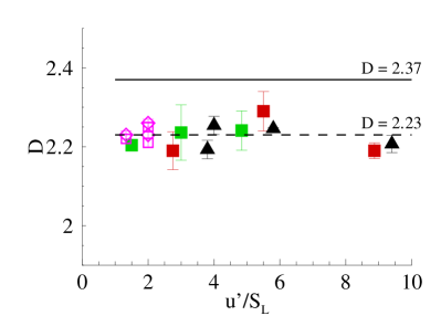
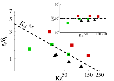
Figure 6: Left panel: fractal dimension D vs turbulent fluctuation intensity $u^{\prime}$ normalised by $S_{L}$. Error bars report the fitting error. Open symbols, DNS: $D$ directly extracted from 3D iso-surfaces ($c=0.5$) by diamond and $D=D_{2}+1$ extracted from 2D cuts of the iso-surfaces ($c=0.5$) containing the jet axis by triangles; closed symbols, experiments where $D=D_{2}+1$ is obtained by 2D cuts containing the jet axis. Thick continuous line, fractal dimension of non-reacting scalar turbulent iso-surfaces, i.e. $D=2.37$. Dashed line, $D=2.23$ present fit of the fractal dimension. Right panel: inner cut-off ($\epsilon_{i}/\delta_{L}$) vs Karlovitz number $Ka$. Only experimental values have been reported since DNSs do not cover a sufficiently wide range of $Ka$. Dotted line represents the scaling $\epsilon_{i}/\delta_{L}\propto Ka^{-1/2}$. In the inset the inner cut-off length normalized by the Kolmogorov scale, $\epsilon_{i}/\eta$, is reported against Karlovitz number. The dash-dotted line represent the constant fitting value $\epsilon_{i}/\eta=10.$

Concerning the inner cut-off length $\epsilon_{i}$, two different scaling are supposed to exist: It may scale either with the Kolmogorov dissipative length $\eta_{k}$ or with the laminar flame thickness $\delta_{L}$. Normalising the inner cut-off length by the laminar flame thickness $\delta_{L}$, it holds:

$${\epsilon_{i}}/{\delta_{L}}\propto Ka^{\beta},$$ (10)

where $\beta=0$ indicates $\epsilon_{i}\propto\delta_{L}$, while $\beta=-1/2$ denotes the scaling of the inner cut-off proportional to the Kolmogorov length. In the right panel of figure 6 we report the scaling of ${\epsilon_{i}}/{\delta_{L}}$ for the experimental dataset. The scaling with $\beta=-1/2$ appears to best fit the data. In particular, the curve $Ka^{-1/2}$ almost perfectly correlates to homogeneous data denoted by the same symbol. These groups correspond to the same experimental conditions concerning the turbulence features $\eta$, $u^{\prime}$ and $Re$, but differ for the equivalence ratio which controls $S_{L}$ and $\delta_{L}$. Hence, even with $Ka=(\delta_{L}/\eta)^{2}>1$, we found a cut-off length proportional to the Kolmogorov scale $\eta$, i.e. $\epsilon_{i}\propto\eta$, but showing values of the order or larger than the corresponding flame thickness, i.e. $\epsilon_{i}\geq\delta_{L}$. This is cleared in the inset of the right panel of figure 6 where the inner cut-off rescaled by the Kolmogorov length $\epsilon_{i}/\eta$ appears almost constant for all the cases with a value around $\epsilon_{i}/\eta\simeq 10$.
This peculiar behaviour can be explained considering that the fractal wrinkling of the flame front is produced by the turbulent self-similar eddies characterising the Kolmogorov inertial range (-5/3 law). Hence it is expected that the fractal features of the flame wrinkling are lost at the end of the inertial range. As shown by the data reported in [42] (see fig. 9 of the paper) the Kolmogorov’s universal scaling of the inertial range (-5/3 law) is actually lost at a scale $\ell$, here referred as ‘limit scale’, proportional to the Kolmogorov length $\eta$, although significantly larger. Specifically, from the power spectra reported in [42] we can estimate this ‘limit scale’ as $2\pi\eta/\ell=0.3\div 0.6$, i.e. $\ell\simeq 10\div 20\eta$, meaning that the self-similar inertial range is actually lost at about $10\div 20$ Kolmogorov length. Concerning our dataset, we found that up to the highest Karlovitz number here investigated, i.e. $Ka=150$, the inner cut-off of the fractal flame front is lost when $\epsilon_{i}\simeq 10\eta\simeq\ell$. It should be noted, that the present dataset cannot shed light on what happens at very high $Ka$ where the typical velocity structures of the inertial range can directly interact with the flame front. It is known that increasing even more the Karlovitz number, i.e. $Ka\gg 100$, the local structure of the flame front becomes strongly altered hence thickened, broken or distributed turbulent flames take place [43]. Since the present modelling relies on a local flame structure similar to the laminar flame (flamelet approximation), we guess that in the very high $Ka$ regime the present framework cannot be directly applied.

3 Large-Eddy-Simulations

The results previously discussed on the fractal dimension $D$ and on the inner cut-off $\epsilon_{i}$ will be exploited to perform LES of reactive flows in order to determine the a-posteriori performance of this simple and fast model.

3.1 LES algorithm

The same numerical algorithm previously used for DNS solves the Favre-filtered Low-Mach Navier-Stokes equations,

$$\frac{\partial\bar{\rho}}{\partial t} +\nabla\cdot\left(\bar{\rho}\tilde{\boldsymbol{u}}\right)=0,$$ (11)

$$\frac{\partial\bar{\rho}\tilde{\boldsymbol{u}}}{\partial t} +\nabla\cdotp\left(\bar{\rho}\tilde{\boldsymbol{u}}\otimes\tilde{\boldsymbol{u}}\right)=\nabla\cdot{\boldsymbol{R}}_{sgs}-\nabla\bar{P}+\frac{1}{Re}\boldsymbol{\nabla}\cdot\overline{\Sigma}+\bar{\rho}{\boldsymbol{g}},$$ (12)

$$\frac{\partial\overline{\rho}\tilde{c}}{\partial t} +{\bf\nabla}\cdot(\overline{\rho}\tilde{\bf{u}}\tilde{c})=\nabla\cdot{\boldsymbol{D}}_{sgs}+\rho_{u}S_{L}\Xi|\nabla\tilde{c}|$$ (13)

$$\nabla\cdot\tilde{\bf u} =\frac{1}{p_{0}}\left\{\nabla\cdot{\boldsymbol{T}}_{sgs}+\frac{\gamma-1}{\gamma}Ce\rho_{u}S_{L}\Xi\,|\nabla\tilde{c}|\right.$$ (14)

$$+\left.\frac{1}{Re}\left(\frac{1}{Pr}\nabla\cdot(\overline{k}\nabla\tilde{T})-\frac{Ce}{Sc}\frac{\gamma-1}{\gamma}\nabla\cdot(\overline{\rho{\cal D}}\nabla\tilde{c})\right)\right\}$$ (15)

$$\overline{\rho}=\frac{p_{0}}{1+Ce\frac{\gamma-1}{\gamma}\,\tilde{c}}$$ (16)

where we assumed $Pr=Sc=0.7$ ($Le=1$). The following extra-stress term is originated by applying the filter to the momentum equation (5):

$${\boldsymbol{R}}_{sgs}=-\bar{\rho}\left(\widetilde{\boldsymbol{u}\otimes\boldsymbol{u}}-\tilde{\boldsymbol{u}}\otimes\tilde{\boldsymbol{u}}\right)=-2\overline{\rho}\boldsymbol{I}\left(\frac{k_{sgs}}{3}+\boldsymbol{\nabla}\cdot\tilde{\boldsymbol{u}}\right)+2\,\overline{\rho}\nu_{T}\,\widetilde{\boldsymbol{S}},$$ (17)

with $2k_{sgs}=\widetilde{|{\boldsymbol{u}}|^{2}}-|\tilde{\boldsymbol{u}}^{2}|$. It was modelled by using the Smagorinsky model with shear-improved formulation by [44], rearranged to take into account the variations of density. $\tilde{S}=0.5\left(\nabla\tilde{\boldsymbol{u}}+(\nabla\tilde{\boldsymbol{u}})^{T}\right)$ is the resolved rate of strain tensor and $\nu_{T}=(C_{S}\Delta)^{2}\cdot(|\tilde{S}({\boldsymbol{x}},t)|-|\langle\tilde{S}({\boldsymbol{x}},t)\rangle|)$ is the eddy-viscosity with the constant $C_{S}=0.12$ and the typical cell size $\Delta=\sqrt[3]{r\Delta\theta\Delta r\Delta z}$, for details see [44]. Sub-grid extra-diffusion terms of scalar quantities read,

$${\boldsymbol{D}}_{sgs}=-\bar{\rho}\left(\widetilde{{\boldsymbol{u}}\,c}-\tilde{\boldsymbol{u}}\tilde{c}\right)=-\bar{\rho}D_{T}\nabla\tilde{c}$$ (18)

$${\boldsymbol{T}}_{sgs}=-\bar{\rho}\left(\widetilde{{\boldsymbol{u}}\,T}-\tilde{\boldsymbol{u}}\tilde{T}\right)=-\bar{\rho}\alpha_{T}\nabla\tilde{T}$$ (19)

and the sub-grid diffusivity is assumed proportional to the Smagorinsky eddy-viscosity: $D_{T}=\alpha_{T}=0.7\nu_{T}$, constant turbulent Schmidt and Prandtl numbers. The wrinkling factor in the (13) is modelled using the fractal features here extracted by the numerical and experimental investigation,

$$\Xi(\Delta)=\alpha(\Delta/\epsilon_{i})^{D-2},$$

where $\alpha=1.7$ is assumed together with $D=2.23$ and $\epsilon_{i}=10\eta=10(\nu^{3}/\varepsilon)^{1/4}$ with $\varepsilon$ the turbulent kinetic energy dissipation. The Kolmogorov scale $\eta$ is calculated using filter observables and assuming K41 theory. If the LES filter scale $\Delta$ falls inside the inertial range, the dissipation can be estimated as $\varepsilon\simeq\tilde{u}_{\Delta}^{3}/\Delta$, where the characteristic velocity at scale $\Delta$ is $\tilde{u}_{\Delta}=\tilde{S}\Delta$ with $\tilde{S}$ the filtered strain rate.

Several Large Eddy Simulations concerning premixed round jets at different Reynolds numbers and $U_{b}/S_{L}$ have been performed in order to test the model in different conditions. Firstly, an accurate comparison between DNS and LES data at the Reynolds number $Re=6000$ and corresponding numerical conditions will be presented. The mesh of the LES is obtained reducing by a factor $4$ in each direction the grid points of the corresponding DNS mesh, $N_{\theta}\times N_{r}\times N_{z}=32\times 51\times 140$.
Successively, keeping fixed the model parameters, two LES’ at higher Reynolds numbers and $U_{b}/S_{L}$, i.e. $u^{\prime}/S_{L}$, have been performed in order test the model at conditions close to real applications. In this case LES’ reproduce the experimental configurations of [26] with $Re=U_{b}D/\nu=16000$ (M3) and $Re=24000$ (M2), respectively. Computational domain and mesh coincide in the two cases and are given by: $[\theta_{max}\times R_{max}\times Z_{max}]=[2\pi\times 6.2D\times 17.5D]$ and $N_{\theta}\times N_{r}\times N_{z}=64\times 101\times 700$, respectively. Similarly to the DNS procedure, fully turbulent inflow conditions are provided by a companion LES of a periodic turbulent pipe flow at the same Reynolds number. The adopted resolution is estimated to be 80 and 180 times smaller than what needed for a resolved DNS. However it is expected to be sufficient to well simulate incompressible jets even at higher Reynolds number, i.e. $Re=400000$, where the minimum requirement for mesh size has been found to be the shear length $L_{s}=\sqrt{\varepsilon/{\cal S}^{3}}$ (where ${\cal S}$ is the shear-rate modulus), see [45] for more details on LES of incompressible jets and on their resolution issue. These aspects assure that the turbulence model should properly simulate the turbulent jet dynamics and allow to test the LES performance for combustion.

3.2 LES results

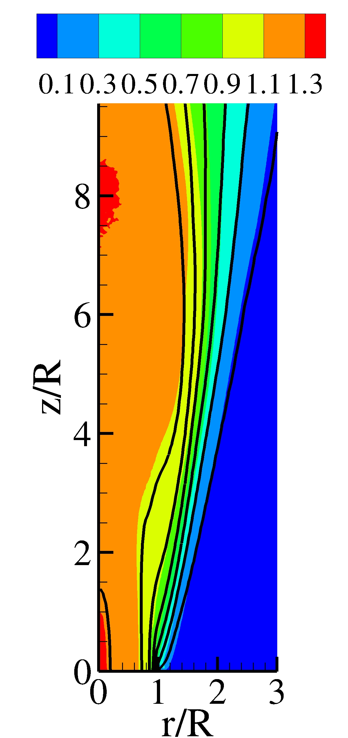
Figure 7: Favre-averaged mean fields of axial velocity $U_{z}/U_{b}$ (left panel), $Y_{R}/Y_{R}^{0}$ (middle panel) and dimensional T (right panel). Contours, DNS with $Re=6000$ and $u^{\prime}/S_{L}=2$; Thick black lines corresponding LES with mesh 4 times coarser in each direction.

A detailed analysis of the LES model performance is carried out replicating the corresponding configuration of the DNS of the premixed Bunsen flame at $Re=6000$ and $u^{\prime}/S_{L}=2$ with a mesh $4^{3}$ times coarser. A general overview of the mean fields is provided in figure 7 where contours represent DNS data and thick black lines the corresponding levels from LES. In the velocity field, the effect of the expansion due to the heat release induces a spread of the mean axial velocity not associated with the typical decay of incompressible jets [37, 45]. The LES model appears to well reproduce this behaviour implying a correct representation of the heat release. In the middle panel the reactant concentration has been presented. The prediction of the flame brush $0<Y_{R}/Y_{R}^{0}<1$, i.e. the region spanned by the instantaneous flame front, is quite remarkable since both the flame height and width are precisely estimated by the LES model. It means that the wrinkling factor $\Xi$ is correctly approximated by the fractal model with $D=2.23$ and $\epsilon_{i}\propto\eta$. The right panel of figure 7, shows the dimensional temperature field ($T_{0}=300\,K$). It should be noted that this Bunsen flame reacts in an open environment, so the temperature iso-levels coincides with the reactant concentration iso-levels only in the inner part of the flame brush where the mixing with the cold environment is negligible. However, further away from the maximum temperature that almost coincides with the adiabatic one, the mixing with the ambient air (entrainment) occurs leading to an additional mixing layer not present in the reactant concentration. As apparent from the plot, the flame brush is correctly captured by the LES model, while small differences are present in the outer mixing layer.

To better analyze the performance of the LES in reproducing DNS data, we report in figure 8 the radial profiles of the same Favre-averaged quantities at four axial stations, $z/D=1;\,2;\,3;\,4$, for DNS and LES. The mean axial velocity $U_{z}/U_{b}$, left column, shows an excellent matching in the whole domain. Profiles of the mean reactant concentration $Y_{R}/Y_{R}^{0}$ –middle column of figure 8– also shows a good agreement. As can be appreciated in figure 7, further downstream, e.g. at $z/D=5$, the mean concentration of reactant is vanishing both for DNS and LES indicating that the flame brush and height are accurately captured by the LES model.

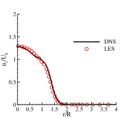
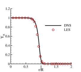
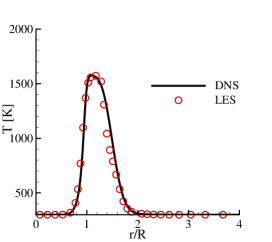
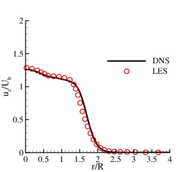
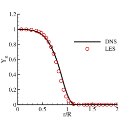
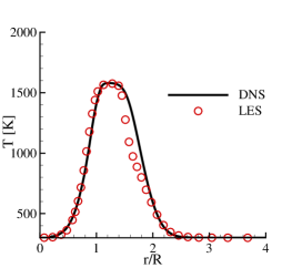
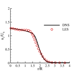
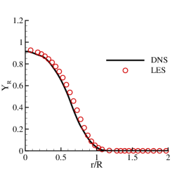
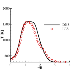
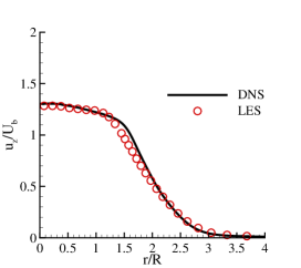
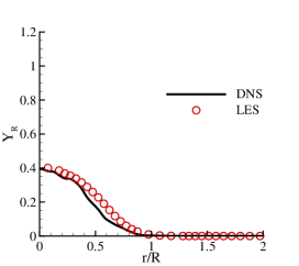
Figure 8: Comparison between LES and DNS at $Re=6000$ and $u^{\prime}/S_{L}=2$. Left column: Favre-averaged axial velocity profiles $U_{z}/U_{b}$; middle column: Favre-averaged reactant profiles normalised by inlet concentration of reactants $Y_{R}/Y_{R}^{0}=1-C/C^{0}$; right column: mean temperature profiles $T$ (dimensional). Rows corresponds to sections at four axial distances, from top: $z/D=1$, $z/D=2$, $z/D=3$, $z/D=4$.

Right-most panels of figure 8 report the mean temperature profiles $T$ (dimensional with $T_{0}=300K$). In each section the temperature shows a maximum almost matching the adiabatic flame temperature ($T_{f}\simeq 1550\,K$) in a region where only burnt gases are present, while for larger radial distances the ambient temperature is approached. Also for this observable, we find a good accordance with DNS data, with small differences present in the mixing region between hot gases and surrounding air where chemical reactions are not present anymore. Actually, the mixing properties in this region show peculiar features that turbulence models often fail to correctly reproduce [46]. In this zone the entrainment of ambient air takes place across a fluctuating intermittent layer which separates the turbulent jet core and the irrotational environment. The non fully turbulent behaviour may be responsible for the deviations we observe in this region.

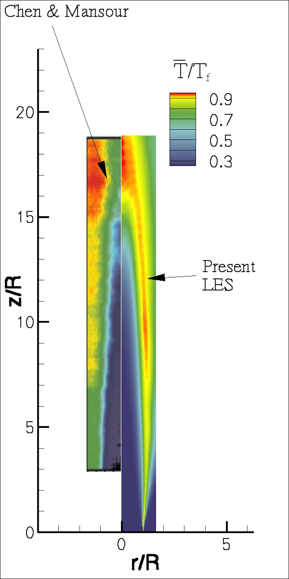
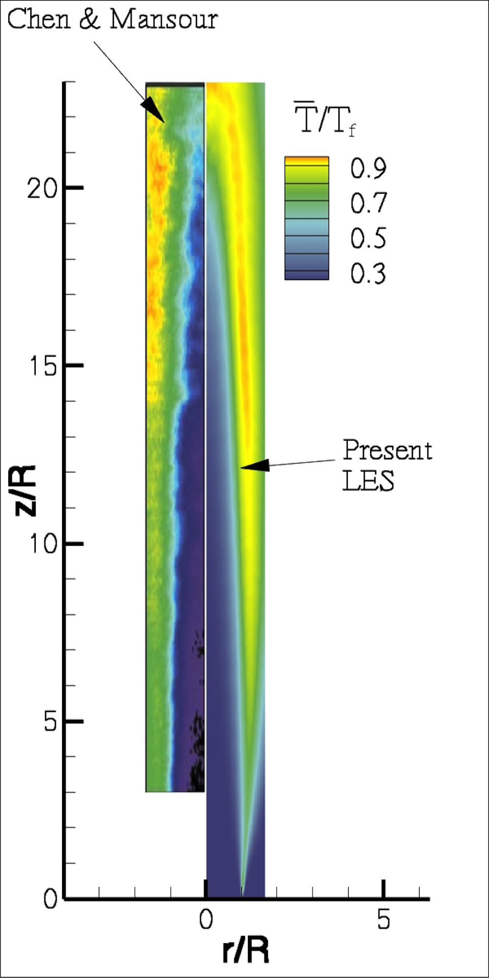
Figure 9: Mean temperature field normalised with the adiabatic flame temperature. Left half-figure: experiments of Chen and Mansour [26]. Right half-figure: present LES computations. Right panel, $Re=16000$, $S_{L}/U_{b}=0.019$; Left panel, $Re=24000$, $S_{L}/U_{0}=0.013$.

To assess the behaviour of the LES at higher Reynolds number we have simulated two turbulent premixed jet flames at $Re=24000$ and $Re=16000$, whose data have been taken from the experiments of [26] on $CH_{4}/Air$ flames (M2 and M3). The ratios between laminar unstretched flame speed and bulk jet velocity are $S_{L}/U_{b}=0.013$ and $S_{L}/U_{b}=0.019$ for the two flames, respectively.
In figure 9, the mean temperature field normalised by the adiabatic flame temperature $T/T_{f}$ is presented (left mid-figures) and compared to that obtained experimentally (right mid-figures). The flame height and width appear correctly estimated by LES. It should be considered that model parameters and mesh size have been kept fixed for the two cases indicating that the present model is sufficiently stable to change of physical conditions. We remark that the present LES mesh is about $80$ and $180$ times smaller than that needed for a resolved DNS at $Re=16000$ and $Re=24000$, respectively. Some differences between experiments and LES are present in the lower part of the shear layer and especially at the flame tip, where the experimental temperatures are lower than those estimated by LES. We attribute these phenomena to local flame stretch and curvature effects induced by the high shear rate, which may modify flame propagation and even lead to local flame extinction, i.e. quenching. This issue has been discussed in details in the work [26] and attributed to the high shear rate typical of these high-Reynolds number flames. Actually, the present LES does not incorporate any ‘sub-model’ able to reproduce the quenching due to a high local value of the shear rate. In the present LES model, a local high shear rate induces a small local Kolmogorov length and hence a high wrinkling factor $\Xi$. It should be noted that it is straightforward to incorporate directly in $\Xi$ a model for the local quenching, e.g. $\Xi=0$ if the local shear rate exceeds a threshold. The issue is out of the scope of the present work, being still under investigation by the present authors.

4 Final remarks

In the present study we investigate the fractal characteristics of turbulent premixed jet flames via a combined approach using DNS and laboratory experiments up to a Karlovitz number $Ka=150$. Experiments on Methane/Air flames consider different inflow geometries, i.e. annular and round Bunsen jets, Reynolds numbers and equivalence ratios. Concerning numerical simulations, a Methane/Air lean mixture has been reproduced by a simple one-step reaction reproducing the fundamental behaviour of a round Bunsen flame. The main flame characteristics as well as its multi-scale fractal structure have been found in good accordance with the experiments.

The fractal dimensions extracted by DNS and experiments has been found almost independent of either the flow configuration or the turbulence features. Its value, $D=2.23$, appears lower than that found for passive scalar isosurfaces (2.37). The fractal scaling is lost at the inner cut-off length, $\epsilon_{i}$ which we observe to scale with the dissipative Kolmogorov length, $\eta$. In particular, we found that the inner cut-off length, $\epsilon_{i}\simeq 10\eta\simeq\ell$, matches with $\ell\sim 10\eta$ which corresponds to the scale where the Kolmogorov’s universal scaling of the inertial range is actually lost [42].

The fractal features, in accordance with previous literature, e.g. [26, 41], have been introduced in a model for LES of turbulent premixed flame in order to estimate the amount of the unresolved flame. Several LES have been performed and compared with reference data. A detailed comparison between LES and corresponding DNS at $Re=6000$ demonstrated the good performance of the model in reproducing the mean flow fields of velocity, temperature and reactants concentration. The LES model has been also tested at higher Reynolds numbers in order to reproduce the mean temperature field of two experiments. Mean flame height and width are remarkably estimated, reflecting a good reproduction of the mean flame evolution. Some differences emerged in the lower part of the shear layer and at the flame tip, pointing out the need for the consideration of flame quenching due to hydrodynamic strain rates and flame stretching, issues which are currently under investigation. Actually the method can be easily extended to account local quenching making null the wrinkling factor $\Xi$ if the local shear rate exceeds a threshold value which depends on the particular fuel mixture. This issue is out of the scope of the present work, being still under investigation, but we aim to show its performance in future works on this topic. In conclusion, the present model shows good performances in a wide range of turbulent flame regimes allowing relatively fast simulations of premixed flames, given its simplicity (algebraic model). It also represents a good framework to incorporate new extensions for accounting more detailed phenomenologies such as local quenching.

References

- [1] J. Driscoll, Turbulent premixed combustion: Flamelet structure and its effect on turbulent burning velocities, Progress in Energy and Combustion Science 34 (1) (2008) 91–134.
- [2] A. Lipatnikov, Fundamentals of premixed turbulent combustion, CRC Press, 2012.
- [3] C. Meneveau, T. Poinsot, Stretching and quenching of flamelets in premixed turbulent combustion, Combust. Flame 86 (1991) 311–332.
- [4] O. Colin, F. Ducros, D. Veynante, T. Poinsot, A thickened flame model for large eddy simulations of turbulent premixed combustion, Physics of Fluids 12 (2000) 1843.
- [5] F. Williams, Turbulent combustion, the Mathematics of combustion (1985) 97–131.
- [6] N. Peters, The turbulent burning velocity for large-scale and small-scale turbulence, Journal of Fluid Mechanics 384 (1999) 107–132.
- [7] H. Pitsch, A consistent level set formulation for large-eddy simulation of premixed turbulent combustion, Combustion and Flame 143 (4) (2005) 587–598.
- [8] E. Knudsen, H. Pitsch, A dynamic model for the turbulent burning velocity for large eddy simulation of premixed combustion, Combustion and Flame 154 (4) (2008) 740–760.
- [9] V. Moureau, B. Fiorina, H. Pitsch, A level set formulation for premixed combustion LES considering the turbulent flame structure, Combustion and Flame 156 (4) (2009) 801–812.
- [10] F. Nicolleau, J. Mathieu, Eddy break-up model and fractal theory: comparisons with experiments, International journal of heat and mass transfer 37 (18) (1994) 2925–2933.
- [11] R. Knikker, D. Veynante, C. Meneveau, A priori testing of a similarity model for large eddy simulations of turbulent premixed combustion, Proceeding of Combustion Institute 29 (2002) 2105–2111.
- [12] B. Mandelbrot, The fractal geometry of nature, Wh Freeman, 1982.
- [13] K. Sreenivasan, C. Meneveau, The fractal facets of turbulence, Journal of Fluid Mechanics 173 (1986) 357–386.
- [14] D. Veynante, L. Vervisch, Turbulent combustion modeling, Progress in Energy and Combustion Science 28 (3) (2002) 193–266.
- [15] M. Boger, D. Veynante, H. Boughanem, A. Trouvé, Direct numerical simulation analysis of flame surface density concept for large eddy simulation of turbulent premixed combustion, in: International Symposium On Combustion, Vol. 1, 1998, pp. 917–926.
- [16] R. Knikker, D. Veynante, C. Meneveau, A dynamic flame surface density model for large eddy simulation of turbulent premixed combustion, Physics of Fluids (1994-present) 16 (11) (2004) L91–L94.
- [17] C. Cohé, F. Halter, C. Chauveau, I. Gökalp, O. L. Gülder, Fractal characterisation of high-pressure and hydrogen-enriched CH4–air turbulent premixed flames, Proceedings of the Combustion Institute 31 (1) (2007) 1345–1352. doi:10.1016/j.proci.2006.07.181.
- [18] O. Chatakonda, E. R. Hawkes, A. J. Aspden, A. R. Kerstein, H. Kolla, J. H. Chen, On the fractal characteristics of low Damköhler number flames, Combustion and Flame 160 (11) (2013) 2422–2433. doi:10.1016/j.combustflame.2013.05.007.
- [19] K. R. Sreenivasan, C. Meneveau, The fractal facets of turbulence, Journal of Fluid Mechanics 173 (1986) 357–386.
- [20] K. R. Sreenivasan, R. Ramshankar, C. Meneveau, Mixing, Entrainment and Fractal Dimensions of Surfaces in Turbulent Flows, Proceeding of the Royal Society of London. Series A, Mathematical and Physical Sciences 421 (1860) (1989) 79–108.
- [21] Ö. L. Gülder, Turbulent premixed combustion modelling using fractal geometry, in: Symposium (International) on Combustion, Vol. 23, Elsevier, 1991, pp. 835–842.
- [22] O. Gülder, G. J. Smallwood, R. Wong, D. R. Snelling, R. Smith, B. Deschamps, J.-C. Sautet, Flame front surface characteristics in turbulent premixed propane/air combustion, Combustion and Flame 120 (4) (2000) 407–416. doi:10.1016/S0010-2180(99)00099-1.
- [23] Ö. L. Gülder, G. J. Smallwood, Inner cutoff scale of flame surface wrinkling in turbulent premixed flames, Combustion and flame 103 (1) (1995) 107–114.
- [24] Y.-C. Chen, M. S. Mansour, Geometric interpretation of fractal parameters measured in turbulent premixed Bunsen flames, Experimental Thermal and Fluid Science 27 (4) (2003) 409–416. doi:10.1016/S0894-1777(02)00254-6.
- [25] R. Knikker, D. Veynante, C. Meneveau, A dynamic flame surface density model for large eddy simulation of turbulent premixed combustion, Physics of Fluids 16 (11) (2004) 91–94. doi:10.1063/1.1780549.
- [26] Y. Chen, M. Mansour, Topology of turbulent premixed flame fronts resolved by simultaneous planar imaging of lipf of oh radical and rayleigh scattering, Experiments in Fluids 26 (1-4) (1999) 277–287.
- [27] G. Troiani, Effect of velocity inflow conditions on the stability of a CH4/air jet-flame, Combustion and Flame 156 (2) (2009) 539–542.
- [28] G. Troiani, M. Marrocco, S. Giammartini, C. Casciola, Counter-gradient transport in the combustion of a premixed CH4/air annular jet by combined PIV/OH-LIF, Combustion and Flame 156 (3) (2009) 608–620.
- [29] F. Picano, F. Battista, G. Troiani, C. Casciola, Dynamics of PIV seeding particles in turbulent premixed flames, Experiments in Fluids 50 (1) (2011) 75–88.
- [30] G. Troiani, F. Battista, F. Picano, Turbulent consumption speed via local dilatation rate measurements in a premixed bunsen jet, Combustion and Flame 160 (10) (2013) 2029–2037.
- [31] P. Perona, J. Malik, Scale-space and edge detection using anisotropic diffusion, Pattern Analysis and Machine Intelligence, IEEE Transactions on 12 (7) (1990) 629–639.
- [32] P. A. M. Kalt, Y.-C. Chen, R. W. Bilger, Experimental investigation of turbulent scalar flux in premixed stagnation-type flames, Combustion and flame 129 (4) (2002) 401–415.
- [33] A. Majda, J. Sethian, The derivation and numerical solution of the equations for zero mach number combustion, Combustion science and technology 42 (3) (1985) 185–205.
- [34] N. Waterson, H. Deconinck, Design principles for bounded higher-order convection schemes–a unified approach, Journal of Computational Physics 224 (1) (2007) 182–207.
- [35] I. Orlanski, A simple boundary condition for unbounded hyperbolic flows, Journal of computational physics 21 (3) (1976) 251–269.
- [36] B. Boersma, G. Brethouwer, F. Nieuwstadt, A numerical investigation on the effect of the inflow conditions on the self-similar region of a round jet, Physics of fluids 10 (1998) 899.
- [37] F. Picano, C. Casciola, Small-scale isotropy and universality of axisymmetric jets, Physics of Fluids 19 (11) (2007) 118106.
- [38] F. Picano, G. Sardina, C. Casciola, Spatial development of particle-laden turbulent pipe flow, Physics of Fluids 21 (2009) 093305.
- [39] F. Battista, F. Picano, G. Troiani, C. Casciola, Intermittent features of inertial particle distributions in turbulent premixed flames, Physics of Fluids 23 (2011) 123304.
- [40] T. Poinsot, D. Veynante, Theoretical and numerical combustion, RT Edwards, Inc., 2005.
- [41] Ö. L. Gülder, G. J. Smallwood, Inner cutoff scale of flame surface wrinkling in turbulent premixed flames, Combustion and flame 103 (1) (1995) 107–114.
- [42] S. G. Saddoughi, S. V. Veeravalli, Local isotropy in turbulent boundary layers at high reynolds number, Journal of Fluid Mechanics 268 (1994) 333–372.
- [43] N. Peters, Turbulent combustion, Cambridge university press, 2000.
- [44] E. Lévêque, F. Toschi, L. Shao, J.-P. Bertoglio, Shear-improved smagorinsky model for large-eddy simulation of wall-bounded turbulent flows, Journal of Fluid Mechanics 570 (2007) 491–502.
- [45] F. Picano, K. Hanjalić, Leray- regularization of the smagorinsky-closed filtered equations for turbulent jets at high reynolds numbers, Flow, turbulence and combustion 89 (4) (2012) 627–650.
- [46] C. B. da Silva, The behavior of subgrid-scale models near the turbulent/nonturbulent interface in jets, Physics of Fluids (1994-present) 21 (8) (2009) 081702.