Observability and controllability of the 1–d wave equation in domains with moving boundary
Abstract.
By mean of generalized Fourier series and Parseval’s equality in weighted –spaces, we derive a sharp energy estimate for the wave equation in a bounded interval with a moving endpoint. Then, we show the observability, in a sharp time, at each of the endpoints of the interval. The observability constants are explicitly given. Using the Hilbert Uniqueness Method we deduce the exact boundary controllability of the wave equation.
Key words and phrases:
Wave equation, non-cylindrical domains, observability, controllability, Hilbert uniqueness method, generalized Fourier series.2010 Mathematics Subject Classification:
35L05, 93B051. Introduction
In this work, we will consider transverse oscillations of a uniform string whose length varies linearly with time. For , we first denote
which is an interval with the right endpoint depending on time. We assume that
| (1.1) |
i.e. the length of is increasing with a constant speed less then . The case of a fixed interval, i.e. and intervals with a fast moving endpoint, , will not be considered here. We prefer to follow Balazs [2] and take the initial time We can take the initial time to be and an initial domain , but this will complicate the mathematics and the Fourier formulas obtained below.
Let and consider the following non-cylindrical domain, and its lateral boundary,
Off course (1.1) ensure the so-called time-likeness condition onfor where is the unit outward normal on the lateral boundary . Let us now consider the following wave equation with homogeneous Dirichlet boundary conditions
| (1.2) |
where is the transverse displacement of the string and the subscripts and stand for the derivatives with respect to time and space, respectively. This is an example of evolution problems in non-cylindrical domains arising in many important applications (such as biology, engineering, quantum mechanics,…), see the survey paper by Knobloch and Krechetnikov [6].
Under the assumption (1.1), it is by now well known that for every initial data
there exists a unique solution to Problem (1.2) such that
see [3, 9]. We define the ”energy” of the above problem as
which is not a conserved quantity in time, in contrast with the wave equation in cylindrical domains.
Let and denote The problem of observability of (1.2) at the boundary can be formulated as follows: To give sufficient conditions on such that there exists for which the following inequality holds for all solutions of (1.2):
| (1.3) |
This is the so-called observability inequality, which allows estimating the energy of solutions in terms of the energy localized at the boundary . The best value of is the observability constant. Due to the finite speed of propagation (here equal to ), the time should be sufficiently large and one expects that it depends on the initial length of and also on the speed of expansion
On the other hand, we consider the following boundary controllability problem: Given
find a control function acting at the boundary such that the solution of
| (1.4) |
satisfies
| (1.5) |
Problem (1.4) admits a unique solution in the sense of transposition, see [12, 11],
To show the controllability, we use the Hilbert Uniqueness Method (HUM) introduced in the seminal work of Lions [10], see also Komornik [7]. The method reduces the controllability problem to the observability of the homogeneous problem (1.2).
The controllability of the wave equation in non-cylindrical domains was considered by several authors. Using the multiplier method, Bardos and Chen [3] derived some decay estimates for the wave equation in time-like domains, then show the exact internal controllability of the wave equation by a stabilization approach. Using a suitable change of variables, Miranda [12] transforms the non-cylindrical domain to a cylindrical one, obtaining a new operator with variable coefficients, then he shows the exact boundary controllability by HUM. Recently, there has been a renewed interest in such controllability problems. In particular, Problem (1.4) was considered, for instance, by [5, 4, 14] where the controllability is established by the multiplier method. Although this is a one-dimensional problem, no one so far, to my knowledge, gave the minimal time of controllability or observability and specified the constant of observability.
Going back to problems in cylindrical domains, the first results of observability and controllability of evolution problems was obtained by Fourier series, see Komornik and Loreti [8], Russell [13] and the references cited therein. This is not the case for non-cylindrical domains. To the author’s knowledge, this paper is the first attempt to apply Fourier series techniques to establish observability and controllability results for the wave equation in non-cylindrical domains. Further results will be presented elsewhere.
In this work, we first express the solution of Problem (1.2) by a Fourier formula, then an estimate of the energy is derived by using Parseval’s equality in a weighted space. In agreement with precedent works, for instance [14], the energy decays as Next, we show that Problem (1.2) is observable at the fixed endpoint of the interval as well as at the moving one. The observability constants are explicitly given and obviously depend on The sharp time of observability, turn out to be the same for both endpoints. Using HUM we obtain the exact boundary controllability, at one of the endpoints, of Problem (1.4) for . This improves some recent results on the controllability of (1.4) obtained by the multiplier method. In particular, taking the initial length and assuming that (1.1) holds,
Sun et al. [14] showed the controllability of (1.4), at the moving endpoint, for . However, they did not address the limiting case and its optimality. Cui et al. [4] obtained a larger time of controllability
The remainder of this paper is organized as follows. In section 2, we give the exact solution of Problem (1.2) then derive a sharp estimate for the energy. Next, the boundary observability and controllability at the fixed endpoint and at the moving endpoint are shown in the third and fourth section, respectively.
2. Energy estimates
2.1. Exact solution
Let such that and consider a nonnegative (weight) function . In the sequel, we denote by the weighted Hilbert space of measurable complex valued functions on endowed by the scalar product
and its associated norm, see for instance Asmar [1]. As usual, we drop in the space notation if .
A well known result in analysis is that the set of functions is a complete orthonormal set in the space By making the change of variable
where , we obtain the set of function which is still a complete orthonormal set in the weighted Hilbert space . Note that (1.1) ensures that the weight function is positive. By consequence, every can be written as
where the coefficients are given by
Moreover, the following Parseval’s equality holds
Arguing as in [2], we can show that the exact solution of Problem (1.2), is the restriction to the interval of the following function given by the generalized Fourier formulas
Note that is an odd function of which ensure that the condition is satisfied for every The coefficients are complex numbers, independent of , given by
where the initial conditions and are also considered as odd functions on defined on the interval .
2.2. Energy estimates
The following lemma gives the decay rate of the energy.
Lemma 1.
Proof.
First, we deduce from the exact formula of the solution that
| (2.3) | |||||
| (2.4) |
which are respectively an odd and an even functions of for every . In particular we deduce that
Thanks to the Parseval’s equality, applied to as a function in the Hilbert space , we have
i.e.
| (2.5) |
Both sides are finite since . Changing by in the last formula, we also obtain
| (2.6) |
Summing up (2.5) and (2.6), we infer that
Since all the functions under the integral signs are even of then
and (2.1) follows. To show (2.2), we use the inequality to obtain
Taking into account (2.1), it comes that
| (2.7) |
This implies (2.2) and the lemma is proved. ∎
3. Observability and controllability at the fixed endpoint.
In this section, we show the observability of (1.2) at , then by applying HUM we deduce the exact controllability of (1.4). First, we can state the following Lemma.
Lemma 2.
Proof.
Remark 2.
From (3.2) we infer that
Then, for any we can always choose an integer such that and since the integrated function is nonnegative, we deduce the following (so-called direct) inequality
| (3.4) |
Noting that , inequality (1.3) reads
hence Lemma 2 is very useful to establish the observability of (1.2) at .
Theorem 1.
Under the assumption (1.1), if Problem (1.2) is observable at the fixed endpoint and it holds that
| (3.5) |
Conversely, if (1.2) is not observable at .
Proof.
Noting that and taking in (3.2), then we get
and thus inequality (3.5) holds for and therefore for any as well.
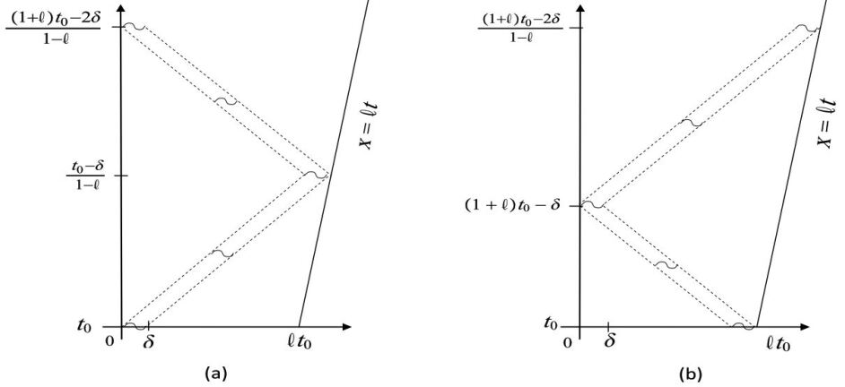
To show that the observability does not hold for , we adapt a proof found in [15] where the wave equation is considered in a fixed interval. Set for some sufficiently small, then solve
| (3.6) |
with data at time with support in the subinterval (see Figure 1a). Let us check that the solution of (3.6) is unique. In one hand, is unique for as it satisfy a wave equation, in an interval expanding at a speed , with initial data at . On the other hand, setting
then is unique as it satisfy a wave equation, in an interval contracting at a speed , with initial data (see [3])
Thus is uniquely determined for This solution is such that for since the segment remains outside the domain of influence of the segment . This means that
and the observability inequality (3.5) does not hold. ∎
Remark 3.
An initial disturbance concentrated near may propagate to the right, as increases, and bounce back on the moving boundary, when is close to then travel to the left to reach the fixed boundary, when is close to , (see Figure 1a). Thus the needed time to complete this journey is close to which is the critical time of observability.
Remark 4.
Let us fix the initial length (by choosing ). Then, as we recover the critical time of observability of the wave equation in the fixed interval
The idea of HUM is based on the equivalence between the observability at of the homogeneous problem (1.2) and the exact controllability at of the non-homogeneous problem (1.4). The proof of this equivalence for the wave equation in an interval with fixed ends (see, for instance, pages 53–57 of [7]) can be carried out without much difficulty to yield the same result for an interval with moving ends. Whence we have the following controllability result.
4. Observability and controllability at the moving endpoint.
In this section, we show the observability and the controllability at . Let us start with the following lemma.
Lemma 3.
Proof.
Remark 6.
Since then In this case, inequality (1.3) reads
Thus Lemma 3 can be used to show the observability at .
Theorem 2.
Under the assumption (1.1), if Problem (1.2) is observable at the moving endpoint and it holds that
| (4.4) |
Conversely, if (1.2) is not observable at .
Proof.
To show that (4.4) does not hold for we argue as above. Consider again for some sufficiently small. Solve Problem (3.6) with data at time with support in the subinterval (see Figure 1b). This solution is such that for since the segment remains outside the domain of influence of the space segment hence
This ends the proof. ∎
Remark 7.
Arguing as in the precedent section, we have the following controllability result.
References
- [1] N. Asmar. Partial differential equations with Fourier series and boundary value problems. Prentice Hall, 2005.
- [2] N. Balazs. On the solution of the wave equation with moving boundaries. J. Math. Anal. Appl., 3:472–484, 1961.
- [3] C. Bardos and G. Chen. Control and stabilization for the wave equation. III: Domain with moving boundary. SIAM J. Control Optim., 19:123–138, 1981.
- [4] L. Cui, X. Liu, and H. Gao. Exact controllability for a one-dimensional wave equation in non-cylindrical domains. J. Math. Anal. Appl., 402:612–625, 2013.
- [5] L. Cui, Y. Jiang, and Y. Wang. Exact controllability for a one-dimensional wave equation with the fixed endpoint control. Bound. Value Probl., 2015(1):1–10, 2015.
- [6] E. Knobloch and R. Krechetnikov. Problems on time-varying domains: Formulation, dynamics, and challenges. Acta Applicandae Math., 137(1):123–157, dec 2014.
- [7] V. Komornik. Exact Controllability and Stabilization. The multiplier method, volume 36 of RMA. Masson–John Wiley & Sons, 1994.
- [8] V. Komornik and P. Loreti. Fourier series in control theory. Springer, 2005.
- [9] J. L. Lions. Quelques méthodes de résolution des problèmes aux limites non linéaires. Dunod-Gautier Villars, 1969.
- [10] J.-L. Lions. Contrôlabilité exacte, stabilisation et perturbations de systemes distribués. Tome 1. Contrôlabilité exacte, volume 8 of RMA. Masson, 1988.
- [11] L. A. Medeiros, M. M. Miranda, and A. T. Lourêdo. Introduction to exact control theory: Method HUM. Editora da Univ. Estadual da Paraيba, 2013.
- [12] M. M. Miranda. Exact controllability for the wave equation in domains with variable boundary. Rev. Mat. Complut., 9(2), 1996.
- [13] D. L. Russell. Controllability and stabilizability theory for linear partial differential equations: recent progress and open questions. SIAM Rev., 20(4):639–739, 1978.
- [14] H. Sun, H. Li, and L. Lu. Exact controllability for a string equation in domains with moving boundary in one dimension. Electron. J. Diff. Equations, 98:1–7, 2015.
- [15] E. Zuazua. Propagation, observation, and control of waves approximated by finite difference methods. SIAM Rev., 47(2):197–243, 2005.