A Model for Paired-Multinomial Data and Its Application to Analysis of Data on a Taxonomic Tree

Abstract

In human microbiome studies, sequencing reads data are often summarized as counts of bacterial taxa at various taxonomic levels specified by a taxonomic tree. This paper considers the problem of analyzing two repeated measurements of microbiome data from the same subjects. Such data are often collected to assess the change of microbial composition after certain treatment, or the difference in microbial compositions across body sites. Existing models for such count data are limited in modeling the covariance structure of the counts and in handling paired multinomial count data. A new probability distribution is proposed for paired-multinomial count data, which allows flexible covariance structure and can be used to model repeatedly measured multivariate count data. Based on this distribution, a test statistic is developed for testing the difference in compositions based on paired multinomial count data. The proposed test can be applied to the count data observed on a taxonomic tree in order to test difference in microbiome compositions and to identify the subtrees with different subcompositions. Simulation results indicate that proposed test has correct type 1 errors and increased power compared to some commonly used methods. An analysis of an upper respiratory tract microbiome data set is used to illustrate the proposed methods.

Keywords: Dirichlet-Multinomial; Microbiome; Paired Multivariate count data; Subcomposition; Subtrees

1 Introduction

The human microbiome includes all microorganisms in and on the human body (Gill et al., 2006). These microbes play important roles in human metabolism in order to maintain human health. Dysbiosis of gut microbiome has been shown to be associated with many human diseases such as obesity, diabetes and inflammatory bowel disease (Turnbaugh et al., 2006; Qin et al., 2012; Manichanh et al., 2012). Next generation sequencing technologies make it possible to quantify the relative composition of microbes in high-throughout. Two high-throughput sequencing approaches have been used in microbiome studies. One approach is based on sequencing the 16S ribosomal RNA (rRNA) amplicons, where the resulting reads provide information about the bacterial taxonomic compositions. Another approach is based on shotgun metagenomic sequencing, which sequences all the microbial genomes presented in the sample, rather than just one marker gene. Both 16S rRNA and shotgun sequencing approaches provide bacterial taxonomic composition information and have been widely applied to human microbiome studies, including the Human Microbiome Project (Turnbaugh et al., 2007) and the Metagenomics of the Human Intestinal Tract project (Qin et al., 2010).

Compared to shotgun metagenomics, 16S rRNA sequencing is an amplicon-based approach, which makes the detection of rare taxa easier and requires less starting genomic material than the metagenomic approaches. One important step in analysis of such 16S amplicon sequencing reads data is to assign them to a taxonomy tree. Several computational methods are available for accurate taxonomy assignments, including BLAST (Altschul et al., 1990), the online Greengenes (DeSantis et al., 2006) and RDP (Cole et al., 2007) classifiers, and several tree-based methods. Liu et al. (2008) compared several of these methods and recommended use of Greengenes or RDP classifier. Each taxonomy assignment method produces lineage assignments at the levels of domain, phylum, class, order, family and genus. The final data can be summarized as counts of reads that are assigned to nodes of a known taxonomic tree.

Given the multivariate nature of the count data measured on the taxonomic tree, methods for analysis of multivariate count data are greatly needed in the microbiome research. Researchers are interested in testing multivariate hypotheses concerning the effects of treatments or experimental factors on the whole assemblages of bacterial taxa. These types of analyses are useful for studies aiming at assessing the impact of microbiota on human health and on characterizing the microbial diversity in general. Multivariate methods for testing the differences in bacterial taxa composition between groups of metagenomic samples have been developed. The commonly used methods include permutation test such as Mantel test (Mantel, 1967), Analysis of Similarity (ANOSIM) (Clarke, 1993), and distance-based MANOVA (PERMANOVA) (Anderson, 2001). An alternative test is based on the Dirichlet multinomial (DM) distribution to model the counts of sequence reads from microbiome samples (La Rosa et al., 2012; Chen and Li, 2013). However, this family of DM probability models may not be appropriate for microbiome data because, intrinsically, such models impose a negative correlation among every pair of taxa. The microbiome data, however, display both positive and negative correlations (Mandal et al., 2015). Models that allow for flexible covariance structures are therefore needed.

Many microbiome studies involve collection of 16S amplicon sequencing data over time or over different body sites in order to assess the dynamics of the microbial communities. Such studies generate paired-multinomial count data, where the repeatedly observed microbiomes and the corresponding taxonomic count data are dependent. Modeling such paired-multinomial count data is the focus of our paper. To the best of our knowledge, there is no flexible model for such paired-multinomial data. In this paper, a probability distribution for paired multinomial count data, which allows flexible covariance structure, is introduced. The model can be used to model repeatedly measured multivariate counts. Based on this paired-multinomial distribution, a test statistic is developed to test the difference of compositions from paired multivariate count data. An application of the test to the analysis of count data observed on a taxonomic tree is developed in order to test difference in paired microbiome compositions and to identify the subtrees with differential subcompositions.

The paper is organized as follows. In Section 2, the Dirichlet multinomial model and the test of compositional equality based on this model are briefly reviewed. A paired multinomial (PairMN) model for paired count data is defined. In Section 3, a statistical test of equal composition based on the paired multinomial model is developed and is applied to count data observed on a taxonomic tree to test for overall compositional difference and to identify the subtrees that show different subcompositions. Results from simulation studies are reported in Section 5 and application to an analysis of gut microbiome data is given in Section 6. A brief discussion is given in Section 7.

2 Paired Multinomial Distribution of Paired Multivariate Count Data

2.1 Dirichlet multinomial distribution for multivariate count data and the associated two-sample test

Consider a set of microbiome samples measured on $n$ subjects, where for each sample, the 16S rRNA sequencing reads are aligned to the nodes of an existing taxonomic tree (Liu et al., 2008) (see Figure 1 (a)). Consider a subtree defined by one internal node of the tree with $d-1$ child nodes. Let $\mathbf{X}_{1},\dots,\mathbf{X}_{n}\in\mathbb{N}^{d}$ denote the $d$-dimensional count data of these $n$ samples, where the $j$th entry of $\mathbf{X}_{i}$ is the number of the sequencing reads aligned to the $j$th child node from the $i$th sample and the last element of $\mathbf{X}_{i}$ is the number of the sequencing reads aligned to the internal node. The following model is developed assuming that $d<n$. Section 4 presents further details on how the model and the test proposed in this Section can be applied to data from the whole taxonomic tree.

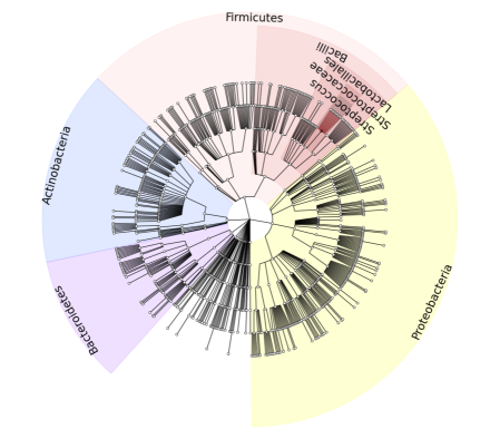
(a)

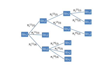
(b)

Figure 1: (a) Taxonomic tree in microbiome studies (generated using GraPhlAn (Asnicar et al., 2015)), where circles from outer to inner are genus, family, order, class, phylum, and kingdom. In our simulations with sparse differential pattern, the count of genus Streptococcus is perturbed to generate the samples from the alternative distribution. As a result, the subtrees with differential subcompositions are the ones with parent node of Kingdom Bacteria, Phylum Firmicutes, Class Bacilli, Order Lactobacillales, Family Streptococcaceae and Genus Streptococcus. (b) An illustration of the probability model of the counts on taxonomic tree, where $\mathbf{X}_{it}^{(1)}=(\mathbf{Q}_{it}(v_{2}),\mathbf{Q}_{it}(v_{3}),\mathbf{Q}_{it}(v_{4}),\mathbf{Q}_{it}(v_{1})-\sum_{j=2}^{4}\mathbf{Q}_{it}(v_{j})),\mathbf{X}_{it}^{(2)}=(\mathbf{Q}_{it}(v_{5}),\mathbf{Q}_{it}(v_{6}),\mathbf{Q}_{it}(v_{2})-\mathbf{Q}_{it}(v_{5})-\mathbf{Q}_{it}(v_{6})),N_{it}^{(1)}=\mathbf{Q}_{it}(v_{1})=\textbf{1}^{\top}\mathbf{X}_{it}^{(1)},N_{it}^{(2)}=\mathbf{Q}_{it}(v_{2})=\textbf{1}^{\top}\mathbf{X}_{it}^{(2)}.$

In order to account for overdispersion of the count data in microbiome studies, $\mathbf{X}_{1},\dots,\mathbf{X}_{n}$ are often assumed to follow a Dirichlet multinomial distribution (La Rosa et al., 2012; Chen and Li, 2013), $DM(N_{i},\boldsymbol{\alpha},\theta),i=1,\cdots,n$, where $N_{i}$ is the total number of the reads from the $i$th sample that are mapped to these $d$ taxa, $\boldsymbol{\alpha}=(\alpha_{1},\cdots,\alpha_{d})$, $0\leq\alpha_{j}\leq 1$, $\sum_{j}\alpha_{j}=1$ is a vector of the true subcomposition of the taxa of a given subtree, and $\theta$ is an overdispersion parameter.

Consider the two-group comparison problem, where the count data of two groups of microbiome samples, denoted by $\mathbf{X}_{11},\dots,\mathbf{X}_{n_{1}1}$ for the $n_{1}$ samples in group 1 and $\mathbf{X}_{12},\dots,\mathbf{X}_{n_{2}2}$ for the $n_{2}$ samples in group 2 are given. Assuming $n_{1},n_{2}>d$, La Rosa et al. (2012) assume each independently follows a DM distribution with

$$\begin{split}&\mathbf{X}_{i1}\sim DM(N_{i1},\boldsymbol{\alpha}_{1},\theta_{1}),i=1,\dots,n_{1},\\ &\mathbf{X}_{i2}\sim DM(N_{i2},\boldsymbol{\alpha}_{2},\theta_{2}),i=1,\dots,n_{2},\end{split}$$ (1)

and propose a test for the following hypothesis of equal subcomposition:

$$H_{0}:\boldsymbol{\alpha}_{1}=\boldsymbol{\alpha}_{2}\mbox{ vs }H_{a}:\boldsymbol{\alpha}_{1}\neq\boldsymbol{\alpha}_{2}.$$ (2)

Define

$$\hat{\boldsymbol{\pi}}_{t}=(\sum_{i=1}^{n_{t}}\mathbf{X}_{it})/(\sum_{i=1}^{n_{t}}N_{it}),t=1,2,$$ (3)

which is a consistent estimator for $\boldsymbol{\alpha}_{t}$ for $t=1,2$. Wilson (1989) and La Rosa et al. (2012) proposed to reject the null hypothesis when

$$\sum_{k=1}^{d}\dfrac{(\hat{\pi}_{1k}-\hat{\pi}_{2k})^{2}}{C_{1}\hat{\pi}_{1k}+C_{2}\hat{\pi}_{2k}}>{\chi^{2}_{d-1}}^{-1}(1-\alpha),$$ (4)

where

$$C_{t}=\dfrac{1}{N_{\cdot t}^{2}}\Big{(}\hat{\theta}_{\alpha_{t}}\big{(}\sum_{i=1}^{n_{t}}N_{it}^{2}-N_{\cdot t}\big{)}+N_{\cdot t}\Big{)},\quad t=1,2$$

and $\hat{\theta}_{t}$ is a consistent estimator of $\theta_{t},t=1,2$.

In many microbiome studies, microbiome data are often observed for the same subjects over two different time points or different body sites. If the microbiome of each subject is measured several times, these repeated measurements are not independent to each other and cannot be handled by the independent DM model. Thus, a new model is developed in the next section to take into account the within subject correlations.

2.2 Paired Multinomial Distribution for Paired Multinomial Data

Any model for paired multinomial data such as those observed in microbiome studies with repeated measures needs to account for the dependency of the data. For a paired multinomial random variable $\mathbf{X}_{i}=(\mathbf{X}_{i1},\mathbf{X}_{i2})\in\mathbb{N}^{d\times 2},i=1,\dots,n$, a paired multinomial (PairMN) distribution can be defined as

$$\mathbf{X}_{i}\sim\mbox{PairMN}\big{(}N_{i1},N_{i2},\boldsymbol{\pi}_{1},\boldsymbol{\pi}_{2},\boldsymbol{\Sigma}_{1},\boldsymbol{\Sigma}_{2},\boldsymbol{\Sigma}_{12}\big{)},$$

where

$$\begin{split}\mathbf{X}_{it}|\mathbf{P}_{it}&\sim~{}\mbox{Multinomial}(N_{it},\mathbf{P}_{it})\in\mathbb{R}^{d},\\ \mathbb{E}\mathbf{P}_{it}&=~{}\boldsymbol{\pi}_{t},\\ \text{Var}\mathbf{P}_{it}&=~{}\boldsymbol{\Sigma}_{t},\\ \text{Cov}(\mathbf{P}_{i1},\mathbf{P}_{i2})&=~{}\boldsymbol{\Sigma}_{12},\end{split}$$ (5)

for $t=1,2$. Here, the group-specific subcomposition is represented by $\boldsymbol{\pi}_{t}$. The joint distribution of $(\mathbf{P}_{i1},\mathbf{P}_{i2})$ is only defined up to its first and second moments so that it includes a wide range of distributions.

Under this probability model, the moments of $\mathbf{X}_{it}$ are given as follow:

$$\begin{split}\mathbb{E}\mathbf{X}_{it}&=~{}N_{it}\boldsymbol{\pi}_{t},\\ \text{Var}\mathbf{X}_{it}&=~{}N_{it}\big{(}diag(\boldsymbol{\pi}_{t})-\boldsymbol{\pi}_{t}\boldsymbol{\pi}_{t}^{\top}\big{)}+N_{it}(N_{it}-1)\boldsymbol{\Sigma}_{t},\\ \text{Cov}(\mathbf{X}_{i1},\mathbf{X}_{i2})&=~{}N_{i1}N_{i2}\boldsymbol{\Sigma}_{12}.\end{split}$$ (6)

Compared to the DM model in (1), this model has several important features. First, for a given $t$, the model allows a more flexible covariance structure for the observed counts that is characterized by $\boldsymbol{\Sigma}_{t}$. Second, this model uses $\boldsymbol{\Sigma}_{12}$ to quantify the correlation between the repeated samples of the same subject. If $\mathbf{P}_{it}$ is assumed to follow a Dirichlet distribution, the proposed model in (5) becomes the DM distribution in (1). However, a parametric assumption is not needed to achieve the flexible covariance structure.

3 Statistical Test Based on Paired Multinomial Samples

For a given subtree of $d$ taxa, in order to test if there is any difference in microbiome subcompositions between two correlated samples, consider the following hypotheses:

$$H_{0}:\boldsymbol{\pi}_{1}=\boldsymbol{\pi}_{2}\mbox{ vs }H_{a}:\boldsymbol{\pi}_{1}\neq\boldsymbol{\pi}_{2}.$$ (7)

Define

$$\hat{\boldsymbol{\pi}}_{t}=\dfrac{\sum_{i=1}^{n}\mathbf{X}_{it}}{\sum_{i=1}^{n}N_{it}},$$

then $\mathbb{E}\hat{\boldsymbol{\pi}}_{t}=\boldsymbol{\pi}_{t}$. A Hotelling’s $T^{2}$ type of statistic based on $\hat{\boldsymbol{\pi}}_{1}-\hat{\boldsymbol{\pi}}_{2}$ can then be developed.

Assume that the sample size $n$ is greater than the number of bacterial taxa $d$ considered. A consistent estimator for $\boldsymbol{\Sigma}_{\hat{\pi}}=\text{Var}\left(\hat{\boldsymbol{\pi}}_{1}-\hat{\boldsymbol{\pi}}_{2}\right)$ is given in the following Lemma.

Lemma 1

Define

$$\begin{split}N_{\cdot t}&=\sum_{i=1}^{n}N_{it}\\ N_{ct}&=\dfrac{1}{(n-1)N_{\cdot t}}\left(N_{\cdot t}^{2}-\sum_{i=1}^{n}N_{it}^{2}\right)\\ \mathbf{S}_{t}&=\dfrac{1}{n-1}\sum_{i=1}^{n}N_{it}(\hat{\boldsymbol{\pi}}_{it}-\hat{\boldsymbol{\pi}}_{t})(\hat{\boldsymbol{\pi}}_{it}-\hat{\boldsymbol{\pi}}_{t})^{\top}\\ \mathbf{G}_{t}&=\dfrac{1}{N_{\cdot t}-n}\sum_{i=1}^{n}N_{it}\big{(}diag(\hat{\boldsymbol{\pi}}_{it})-\hat{\boldsymbol{\pi}}_{it}\hat{\boldsymbol{\pi}}_{it}^{\top}\big{)}\\ \widehat{\boldsymbol{\Sigma}}_{12}&=\dfrac{1}{(n-1)}\sum_{i=1}^{n}\dfrac{N_{i1}+N_{i2}}{N_{c1}+N_{c2}}(\hat{\boldsymbol{\pi}}_{i1}-\hat{\boldsymbol{\pi}}_{1})(\hat{\boldsymbol{\pi}}_{i2}-\hat{\boldsymbol{\pi}}_{2})^{T}\end{split}$$

where $\hat{\boldsymbol{\pi}}_{it}=\mathbf{X}_{it}/N_{it}$. Assuming $N_{it}$’s are bounded by a common fixed number $N$ for all $i$ and $t$, then

$$\begin{split}\widehat{\boldsymbol{\Sigma}}_{\hat{\pi}}=&\sum_{t=1}^{2}\left\{\dfrac{\mathbf{S}_{t}+(N_{ct}-1)\mathbf{G}_{t}}{N_{ct}N_{\cdot t}}+\dfrac{\sum_{i=1}^{n}N_{it}^{2}-N_{\cdot t}}{N_{ct}N_{\cdot t}^{2}}(\mathbf{S}_{t}-\mathbf{G}_{t})\right\}\\ &-\dfrac{\sum_{i=1}^{n}N_{i1}N_{i2}}{N_{\cdot 1}N_{\cdot 2}}\big{(}\widehat{\boldsymbol{\Sigma}}_{12}+\widehat{\boldsymbol{\Sigma}}_{12}^{\top}\big{)}\end{split}$$ (8)

is a consistent estimator of $\boldsymbol{\Sigma}_{\hat{\pi}}=\text{Var}\left(\hat{\boldsymbol{\pi}}_{1}-\hat{\boldsymbol{\pi}}_{2}\right)$. In other words,

$$||\widehat{\boldsymbol{\Sigma}}_{\hat{\pi}}-\boldsymbol{\Sigma}_{\hat{\pi}}||_{\max}\rightarrow 0\mbox{ in probability as }n\rightarrow\infty$$ (9)

where $||\cdot||_{\max}$ is the max norm of a matrix.

Since $\widehat{\boldsymbol{\Sigma}}_{\hat{\pi}}$ is singular due to the unit sum constraint on $\mathbf{P}_{it}$, a statistic to test $H_{0}$ vs $H_{a}$ specified in (7) is defined as

$$F=\dfrac{n-d+1}{(n-1)(d-1)}(\hat{\boldsymbol{\pi}}_{1}-\hat{\boldsymbol{\pi}}_{2})\widehat{\boldsymbol{\Sigma}}_{\hat{\pi}}^{\dagger}(\hat{\boldsymbol{\pi}}_{1}-\hat{\boldsymbol{\pi}}_{2})^{\top},$$ (10)

where $\widehat{\boldsymbol{\Sigma}}_{\hat{\pi}}^{\dagger}$ is the Moore-Penrose pseudoinverse of $\widehat{\boldsymbol{\Sigma}}_{\hat{\pi}}$. The Moore-Penrose pseudoinverse is chosen over other forms of pseudoinverse because of its simple expression related to the singular values of the original matrix and inverted matrix. Since $\widehat{\boldsymbol{\Sigma}}_{\hat{\pi}}$ is not guaranteed to be non-negative definite, the negative eigenvalues of $\widehat{\boldsymbol{\Sigma}}_{\hat{\pi}}$ are truncated to 0 in the computation, however, the truncation does not affect the convergence of $\widehat{\boldsymbol{\Sigma}}_{\hat{\pi}}$.

The following theorem shows that under the null, the test statistic defined in (10) follows an asymptotic $F$-distribution with degrees of freedom of $d-1$ and $n-d-1$.

Theorem 1

With test statistic $F$ defined in (10), an asymptotic level $\alpha$ test for testing (7) is to reject $H_{0}$ when

$$F>F_{d-1,n-d+1}^{-1}(1-\alpha).$$ (11)

The $p$-value for testing (7) is

$$p=1-F_{d-1,n-d+1}(F).$$ (12)

Remark 1

Lemma 1 and the proposed test statistic in (10) can be easily extended to unpaired multivariate count data with unequal sample sizes. Specifically, $\widehat{\boldsymbol{\Sigma}}_{\hat{\pi}}$ in (8) can be replaced by

$$\widehat{\boldsymbol{\Sigma}}_{\hat{\pi}}=\sum_{t=1}^{2}\left\{\dfrac{\mathbf{S}_{t}+(N_{ct}-1)\mathbf{G}_{t}}{N_{ct}N_{\cdot t}}+\dfrac{\sum_{i=1}^{n}N_{it}^{2}-N_{\cdot t}}{N_{ct}N_{\cdot t}^{2}}(\mathbf{S}_{t}-\mathbf{G}_{t})\right\}$$

and $\mathbf{S}_{t}$, $\mathbf{G}_{t}$, $N_{\cdot t}$ and $N_{ct}$ within each group $t$ can be calculated in the same fashion as Lemma 1.

4 Analysis of Microbiome Count Data Measured on the Taxonomic Tree

This section presents details of applying the proposed F-test in Theorem 1 for paired-multinomial data to analysis of 16 S data. Our goal is to identify the subtrees of a given taxonomic tree that show differential subcomposition between two repeated measurements and to perform a global test of overall microbiome composition between two conditions. A global probability model for count data on a taxonomic tree is first introduced.

4.1 A global probability model for count data on a taxonomic tree

A rooted taxonomic tree $T$ with nodes $v_{1},\dots,v_{K_{0}}$ representing for the taxonomic units of $T$ is often available based on 16S sequencing data. For each microbiome sample, the 16S reads can be aligned to the nodes of $T$ to output the count of reads assigned to each node. Without loss of generality, assume that the first $K$ nodes $v_{1},\dots,v_{K}$ are all the internal non-leaf nodes and $v_{1}$ is the root node. Also, denote $\tau(v_{k})$ as the set of all direct child nodes of $v_{k},k=1,\dots,K$. Figure  1 (b) presents a tree to illustrate the setup.

For a given internal node $v_{k}$, let $\mathbf{Q}(v_{k})$ be the sum of number of reads assigned to $v_{k}$ and the number of reads assigned to all its descending nodes. For example, if $v_{k}$ corresponds to the phylum Firmicutes, $\mathbf{Q}(v_{k})$ is the count of all reads assigned to Firmicutes and all classes that belong to Firmicutes. For convenience, denote $\mathbf{Q}(S)=\big{(}\mathbf{Q}(v_{k_{1}}),\dots,\mathbf{Q}(v_{k_{j}})\big{)}$ for any set of nodes $S=\{v_{k_{1}},\dots,v_{k_{j}}\}$. For each split from a parental node to the child nodes, the reads on the parent node are either assigned to a child node or remain unassigned. For each parent node $v_{k}$, let the vector $\mathbf{Q}(\tau(v_{k}))$ denote the counts of reads assigned to its direct child nodes and $\mathbf{Q}(v_{k})-\sum_{j\in\tau(v_{k})}\mathbf{Q}(v_{j})$ be the count of reads that can only be assigned to $v_{k}$. For a subject $i$ with measurement index $t$, at a given internal node $v_{k}$, $k=1,\dots,K$, denote

$$\begin{split}\mathbf{X}_{it}^{(k)}&=\big{(}\mathbf{Q}_{it}(\tau(v_{k})),\mathbf{Q}_{it}(v_{k})-\sum_{j:v_{j}\in\tau(v_{k})}\mathbf{Q}_{it}(v_{j})\big{)}^{\top},\\ N_{it}^{(k)}&=\mathbf{Q}_{it}(v_{k})=\textbf{1}^{\top}\mathbf{X}_{it}^{(k)},\end{split}$$ (13)

where $N_{it}^{(k)}$ is the sum of these read counts.

For a repeated microbiome study, $\mathbf{Q}_{i1}(T)$ and $\mathbf{Q}_{i2}(T)$ represent the counts assigned to the nodes of the tree $T$. These count data are assumed to be generated hierarchically, conditioning on the total read count of each internal node. At each internal node $v_{k}$, $k=1,\dots,K$, given the total counts $(\mathbf{Q}_{i1}(v_{k}),\mathbf{Q}_{i2}(v_{k}))=(N_{i1}^{(k)},N_{i2}^{(k)})$, the paired vectors of read counts

$$(\mathbf{X}_{i1}^{(k)},\mathbf{X}_{i2}^{(k)})=$$

$$\Big{(}\big{(}\mathbf{Q}_{i1}(\tau(v_{k})),\mathbf{Q}_{i1}(v_{k})-\sum_{j:v_{j}\in\tau(v_{k})}\mathbf{Q}_{i1}(v_{j})\big{)}^{\top},\big{(}\mathbf{Q}_{i2}(\tau(v_{k})),\mathbf{Q}_{i2}(v_{k})-\sum_{j:v_{j}\in\tau(v_{k})}\mathbf{Q}_{i2}(v_{j})\big{)}^{\top}\Big{)}$$

is assumed to follow a PairMN distribution

$$\begin{split}(\mathbf{X}_{i1}^{(k)},\mathbf{X}_{i2}^{(k)})|(N_{i1}^{(k)},N_{i2}^{(k)})\sim\mbox{PairMN}\big{(}N_{i1}^{(k)},N_{i2}^{(k)},\boldsymbol{\pi}^{(k)}_{1},\boldsymbol{\pi}^{(k)}_{2},\boldsymbol{\Sigma}^{(k)}_{1},\boldsymbol{\Sigma}^{(k)}_{2},\boldsymbol{\Sigma}_{12}^{(k)}\big{)}.\end{split}$$ (14)

As an illustration, for the tree in Figure 1 (b), the parameters associated with subtree under node $v_{1}$ are $\boldsymbol{\pi}_{t}^{(1)}=\mathbb{E}\left[\mathbf{X}_{it}^{(1)}/N_{it}^{(1)}\big{|}N_{it}^{(1)}\right]$, which represent the subcomposition of nodes $v_{2}$ to $v_{4}$ and taxa can not be further assigned. Similarly $\boldsymbol{\pi}_{t}^{(2)}=\mathbb{E}\left[\mathbf{X}_{it}^{(2)}/N_{it}^{(2)}\big{|}N_{it}^{(2)}\right]$ characterizes the subcomposition of nodes $v_{5}$ and $v_{6}$ under the subtree of node $v_{2}$.

4.2 Identification of subtrees of with differential subcompositions based on the proposed test

In order to identify the subtrees with differential subcompositions between the two measurements, the following hypotheses are tested using the F-test in Theorem 1,

$$H_{0}^{(k)}:\boldsymbol{\pi}_{1}^{(k)}=\boldsymbol{\pi}_{2}^{(k)},\quad k=1,\dots,K.$$ (15)

Define $p_{k}$ as the $p$-value from testing $H_{0}^{(k)}$. Theorem 1 shows that under the null hypotheses, $p_{k}$’s are asymptotically uniformly distributed. In fact, they are also asymptotically independent under the null. Take Figure 1 (b) as an example, under the $H_{0}^{(1)}$ and $H_{0}^{(2)}$,

$$\begin{split}\mathbb{P}(p_{1}\leq\alpha,p_{2}\leq\beta)&=\int\mathbb{P}(p_{1}\leq\alpha|\mathbf{Q}(v_{2}),p_{2}\leq\beta)\mathbb{P}(p_{2}\leq\beta|\mathbf{Q}(v_{2}))dF(\mathbf{Q}(v_{2}))\\ &=\int\mathbb{P}(p_{1}\leq\alpha|\mathbf{Q}(v_{2}))\mathbb{P}(p_{2}\leq\beta|\mathbf{Q}(v_{2}))dF(\mathbf{Q}(v_{2}))\\ &\stackrel{{\scriptstyle a}}{{=}}\beta\int\mathbb{P}(p_{1}\leq\alpha|\mathbf{Q}(v_{2}))dF(\mathbf{Q}(v_{2}))\\ &=\beta\mathbb{P}(p_{1}\leq\alpha)\stackrel{{\scriptstyle a}}{{=}}\mathbb{P}(p_{1}\leq\alpha)\times\mathbb{P}(p_{2}\leq\beta),\end{split}$$

where $\stackrel{{\scriptstyle a}}{{=}}$ represents equation that holds asymptotically. Therefore, to control for multiple comparisons, the false discovery rate (FDR) procedure (Benjamini and Hochberg, 1995) can be used to identify the subtrees with different subcompositions between two repeated measurements.

4.3 Global test for differential overall compositions on taxonomic tree

The goal for testing the global difference in taxonomic composition between a pair of measurements can be formulated as the following composite hypothesis,

$$H_{0}:\boldsymbol{\pi}_{1}^{(k)}=\boldsymbol{\pi}_{2}^{(k)},k=1,\cdots,K\quad\mbox{vs}\quad H_{a}:\boldsymbol{\pi}_{1}^{(k)}\neq\boldsymbol{\pi}_{2}^{(k)},\mbox{for at least one $k$}.$$ (16)

As shown in previous section, under the $H_{0}$, $p$-values for testing $H_{0}^{(k)}$ for $k=1,\cdots,K$ are independent. In addition, the number of tests $K$ is determined by the prior taxonomic tree and does not depend on the sample size $n$. To test this composite hypothesis (16), a combined $p$-value can be obtained using the Fisher’s method,

$$p_{combined}=1-(\chi^{2}_{2K})^{-1}\left(-2\sum_{k=1}^{K}\log p_{k}\right).$$ (17)

Alternatively, let $p_{(2)}$ be the $2^{nd}$ smallest $p$-value of $p_{1},\dots,p_{K}$, a statistic based on this $2^{nd}$ smallest $p$-value,

$$p_{combined}=1-\big{[}1+(K-1)p_{(2)}\big{]}(1-p_{(2)})^{K-1}$$ (18)

can also be used, where (18) is a special case of Wilkinson’s method of $p$-value combination (Wilkinson, 1951) summarized by Zaykin et al. (2002). Under the null, the $p_{combined}$ computed using either method is asymptotically uniformly distributed. Test (18) is more powerful if only a small number of subtrees show differential subcomposition between the two measurements, while test (17) is more suitable if the differences occur in a large number of subtrees.

5 Simulation Studies

5.1 Comparison with test based on the DM model

To compare the performance of our pairMN test statistic in (11) with the original unpaired statistic (4), two data generating models within the class of PairMN are considered. The first model generates $\mathbf{P}_{it},i=1,\dots,n$ based on a mixture of Dirichlet distributions:

$$\begin{split}&\mathbf{P}_{it}=(1-\rho)\mathbf{P}_{it}^{\prime}+\rho\mathbf{P}_{i}^{\prime\prime},\quad t=1,2,\\ &\mathbf{P}_{it}^{\prime}\sim\mbox{Dir}(\boldsymbol{\alpha}_{t},\theta_{\alpha_{t}}),\quad t=1,2,\\ &\mathbf{P}_{i}^{\prime\prime}\sim\mbox{Dir}(\boldsymbol{\ell},\theta_{\ell}).\end{split}$$ (19)

Under this setting,

$$\begin{split}\boldsymbol{\pi}_{t}&=~{}(1-\rho)\boldsymbol{\alpha}_{t}+\rho\boldsymbol{\ell},\quad 0<\rho<1,\quad t=1,2\\ \boldsymbol{\Sigma}_{t}&=~{}(1-\rho)^{2}\theta_{\alpha_{t}}\big{(}diag(\boldsymbol{\alpha}_{t})-\boldsymbol{\alpha}_{t}\boldsymbol{\alpha}_{t}^{\top}\big{)}+\rho^{2}\theta_{\ell}\big{(}diag(\boldsymbol{\ell})-\boldsymbol{\ell}\boldsymbol{\ell}^{\top}\big{)},\quad t=1,2\\ \boldsymbol{\Sigma}_{12}&=~{}\rho^{2}\theta_{\ell}\big{(}diag(\boldsymbol{\ell})-\boldsymbol{\ell}\boldsymbol{\ell}^{\top}\big{)}.\\ \end{split}$$ (20)

In our simulation, the dimension is set as $d=8$. The parameter $\rho$ is used to control the degree of correlation in $\boldsymbol{\Sigma}_{12}$, where $\rho$ ranges from 0 to 0.6. Other parameters are set as $\theta_{\ell}=1$, $\theta_{\alpha_{1}}=3$, $\theta_{\alpha_{2}}=5$, $\boldsymbol{\ell}=(0.12,0.06,0.08,0.43,0.02,0.14,0.1,0.05)$, $\boldsymbol{\alpha}_{1}$ and $\boldsymbol{\alpha}_{2}$ such that $\boldsymbol{\pi}_{1}=(0.15,0.05,0.22,0.3,0.03,0.1,0.07,0.08)$, and under the alternative hypothesis $\boldsymbol{\pi}_{2}=(0.1,0.1,0.22,0.3,0.03,0.1,0.07,0.08)$. The number of total counts $N_{it}$ are simulated from a Poisson distribution with a mean 1000. When $\rho=0$, this model degenerates to the Dirichlet-multinomial distribution.

The second model generates $\mathbf{P}_{it},i=1,\dots,n$ based on a log-normal distribution. Specifically,

$$\mathbf{P}_{it}=\dfrac{e^{\mathbf{Z}_{it}}}{\boldsymbol{1}^{\top}e^{\mathbf{Z}_{it}}},\quad t=1,2,$$ (21)

where

$$\begin{split}(Z_{i1j},Z_{i2j})&\sim~{}N\left(\left[\begin{array}[]{c}\mu_{j1}\\ \mu_{j2}\end{array}\right],\left[\begin{array}[]{cc}\sigma_{j1}^{2}&\rho\sigma_{j1}\sigma_{j2}\\ \rho\sigma_{j1}\sigma_{j2}&\sigma_{j2}^{2}\end{array}\right]\right),\quad j=1,\dots,d,\\ \mathbf{Z}_{it}&=~{}(Z_{it1},\dots,Z_{itd})^{\top},\quad t=1,2.\end{split}$$

Under this setting, no explicit expressions for $\boldsymbol{\pi}_{t}$, $\boldsymbol{\Sigma}_{t}$ and $\boldsymbol{\Sigma}_{12}$ are available, but the correlation can be quantified using $\rho$, and the difference in $\boldsymbol{\pi}_{t}$ can be quantified by the difference in $\boldsymbol{\mu}_{t}=(\mu_{1t},\dots,\mu_{dt})^{\top},t=1,2$. In our simulation, the dimension of sample is $d=8$, $\rho$ ranges from 0 to 0.6, $\boldsymbol{\sigma}_{t}=(\sigma_{1t},\dots,\sigma_{dt})^{\top}=(1,\dots,1)$ for $t=1,2$, $\boldsymbol{\mu}_{1}=(3,1,0.5,1,0,1,1,0)$, and $\boldsymbol{\mu}_{2}=(3,1,1,0.5,0,1,1,0)$ under the alternative. The number of total counts $N_{it}$ are also simulated from a Poisson distribution with a mean 1000.

For both data generating models, sample sizes of $n=20,50$ and $100$ are considered. The dimension of parameters is chosen to be eight in all simulations to mimic the fact that most of the nodes on the taxonomic tree in our study have less than ten child nodes. The simulations are repeated 5,000 times for each specific setting and the null hypothesis is rejected at level of $\alpha=0.05$. The type I error and the empirical power of the various tests are shown in Figure 2. It shows that both tests have test size under the nominal level in all settings. For data simulated from the paired multinomial-Dirichlet distribution (19), the power of the unpaired test is slightly better than the paired test only when $\rho$ is very small, that is, when there is a weak within-subject correlation (Figure 2 (a)). This is expected since the unpaired test (4) is developed specifically for the Dirichlet-multinomial distribution, i.e. PairMN model with $\rho=0$. When $\rho$ increases from 0 to 0.6, the paired test has a steadily increasing power with the test size still around the nominal level, while the size and power of the unpaired test gradually decrease. The results suggest that compared with the paired test, the unpaired test tends to be conservative and therefore has reduced power in detecting the difference in compositions when the within-subject correlation is large.

For data simulated from log-normal-based PairMN model (21), the power of our paired test is much larger than the power of the unpaired test for all values of $\rho$, while the type 1 errors are well controlled (Figure 2 (b)). These results show that the proposed paired test performs well in both data generating models, suggesting that our test is very flexible and robust to different distributions of $\mathbf{P}_{it}$.

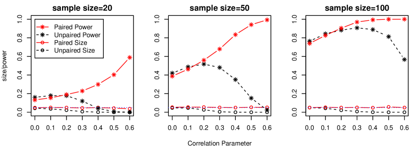
(a) Mixed Dirichlet $P_{it}$.

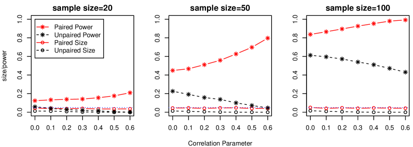
(b) Log-normal based $P_{it}$.

Figure 2: Simulation results: size and power of the paired and unpaired tests for data simulated under the PairMN model (a) and the correlated log-normal model (b) for sample size $n=20,50$ and 100. x-axis is the correlation parameter $\rho$.

5.2 Simulating count data on a taxonomic tree

The proposed tests in (17) and (18) are further compared with PERMANOVA test (Anderson, 2001) using $L^{1}$ Kantorovich-Rubinstein (K-R) distance (Evans and Matsen, 2012) with unit branch length and with each pair of samples as a stratum. Using the notations in Section 4.3, the $L^{1}$ K-R distance between two trees $\mathbf{Q}_{i_{1}t_{1}}$ and $\mathbf{Q}_{i_{2}t_{2}}$ is given by

$$d(\mathbf{Q}_{i_{1}t_{1}},\mathbf{Q}_{i_{2}t_{2}})=\sum_{k=1}^{K_{0}}\left|\mathbf{p}_{i_{1}t_{1}}(v_{k})-\mathbf{p}_{i_{2}t_{2}}(v_{k})\right|$$ (22)

where

$$\mathbf{p}_{it}(v_{k})=\big{(}\mathbf{Q}_{it}(v_{k})-\sum_{j:v_{j}\in\tau(v_{k})}\mathbf{Q}_{it}(v_{j})\big{)}/\mathbf{Q}_{it}(v_{1})\quad k=1,\dots,K_{0}$$

is the proportion of reads that are assigned to node $v_{k}$ but cannot be further specified to its child nodes. This is sum of the $l_{1}$ distances between two compositional vectors over each branch of the taxonomic tree.

In order to simulate data that mimic real microbiome count data, count data on the taxonomic tree are generated based on sampling from a real 16S microbiome dataset from Flores et al. (2014), where the gut (feces), palm and tongue microbial samples of 85 college-age adults were taken in a range of three months and were characterized using 16S rRNA sequencing. Within the gut microbiome samples, counts of reads are summarized on a taxonomic tree that has 1050 nodes from kingdom to species (see Figure 1(a)). Since no large change is expected in gut microbiome during a three-month period, these samples are assumed to have the same null distribution, which results in a total of 638 gut microbial samples. Using the notation in Section 4.2, these samples are denoted as $\mathbf{Q}^{o}_{1},\dots,\mathbf{Q}^{o}_{638}$. The composition matrix matrix $\textbf{P}^{o}\in(0,1)^{638\times 1050}$ with

$$\textbf{P}^{o}(i,k)=\bigg{(}\mathbf{Q}^{o}_{i}(v_{k})-\sum_{j:v_{j}\in\tau(v_{k})}\mathbf{Q}^{o}_{i}(v_{j})\bigg{)}/\mathbf{Q}^{o}_{i}(v_{1}),\quad i=1,\dots,638,\quad k=1,\dots,1050$$

is first calculated, which is the composition of all nodes for each of the 638 gut microbial samples. The total counts of reads of all samples are also calculated and recorded as $\textbf{N}^{o}\in\mathbb{N}^{638}$.

To simulate a pair of correlated microbiome sample $\mathbf{Q}_{i1}$ and $\mathbf{Q}_{i2}$, three compositions $\mathbf{P}^{o}_{i1}$, $\mathbf{P}^{o}_{i2}$ and $\mathbf{P}^{o}_{i3}$ from $\textbf{P}^{o}$ are randomly sampled and two total counts $N^{o}_{i1}$ and $N^{o}_{i2}$ are randomly resampled from $\textbf{N}^{o}$. Read counts $\mathbf{W}_{i1}$ and $\mathbf{W}_{i2}$ are then sampled from multinomial distributions $(N^{o}_{i1},(\mathbf{P}^{o}_{i1}+\mathbf{P}^{o}_{i3})/2)+\mathbf{E}_{i1}$ and $(N^{o}_{i2},(\mathbf{P}^{o}_{i2}+\mathbf{P}^{o}_{i3})/2)+\mathbf{E}_{i2}$, respectively, where $\mathbf{E}_{i1}$ and $\mathbf{E}_{i2}$ are small perturbations to certain nodes of the tree to generate $\mathbf{W}_{i1}$ and $\mathbf{W}_{i2}$ that have different distributions. Two differential abundance patterns are considered:

1. Sparse differential abundance: $\mathbf{E}_{i1}=0$ and $\mathbf{E}_{i2}$ is drawn from Binomial$(N^{o}_{i2},p_{\epsilon})$ at the coordinate corresponding to the genus of Streptococcus and zero otherwise.

2. Dense differential abundance: $\mathbf{E}_{i1}$ is drawn from Binomial$(N^{o}_{i2},p_{\epsilon})$ at the coordinates corresponding to the genera of Streptococcus, Eubacterium, Parabacteroides, and zero otherwise, and $\mathbf{E}_{i2}$ is drawn from Binomial$(N^{o}_{i2},p_{\epsilon})$ at the coordinates corresponding to the genera of Porphyromonas, Moraxella, Ruminococcus, and zero otherwise.

The count vector $\mathbf{Q}_{it}$ is then iteratively computed such that $\mathbf{Q}_{it}(v_{k})-\sum_{j:v_{j}\in\tau(v_{k})}\mathbf{Q}_{it}(v_{j})=\mathbf{W}_{itk}$ for $t=1,2$ and $i=1,\dots,n$, where $n$ is the number of pairs simulated and is set to be 20, 50 and 100 in our simulation. The percent of perturbation $p_{\epsilon}$ is chosen to range from 0 to 2%. For each scenario, the simulations are repeated 100 times. For the global test of (16), the null hypothesis is rejected at the $\alpha$-level of 0.05. For the identification of subtrees with differential subcompositions in multiple testing (15), the FDR is controlled at the 0.05 level.

Figure 3 compares the rejection rate of PERMANOVA with our method using (17) or (18) for the global test (16). For the method (18) that ombines $p$-values using the $2^{nd}$ smallest $p$-value, our paired test based on PairMN in (10) is also compared with the unpaired test based on DM in (4). In the sparse differential abundance setting, when the sample size is small, none of the methods is able to detect the perturbation to Streptococcus. As the sample size increases, the rejection rate of our method using the $2^{nd}$ smallest $p$-value combination of the paired-tests gradually increases, especially when the percent of perturbation gets closer to 2%. Fisher’s method combining $p$-values does not perform as well because the perturbation only occurs to a very small number of subtrees. The method using $2^{nd}$ smallest $p$-value combination of the unpaired tests also performs worse than the paired tests.

In the dense differential abundance setting, all methods are able to detect the perturbations. The test based on DM has the largest power, but also has inflated type I error. Among the other tests, our test based on PairMN with $2^{nd}$ smallest $p$-value performs the best with type I error under control.

(a) Sparse differential pattern setting.

(b) Dense differential pattern setting.

Figure 3: Comparison of rejection rate of the proposed method with PERMANOVA with the level of test at $\alpha=0.05$. x-axis is the perturbation percentage $p_{\epsilon}$, where $p_{\epsilon}=0$ corresponds to the null hypothesis.

Figure 4 (a) shows the percent of discoveries of the differential subtrees with sparse differential pattern and FDR controlled at 0.05. The observed FDR is close to the nominal level of 0.05. Since the count of genus Streptococcus is set to be different, the counts on all the ancestor nodes of Streptococcus are also changed. Therefore, the differential subtrees denoted by their root nodes are: (a) Kingdom Bacteria, (b) Phylum Firmicutes, (c) Class Bacilli, (d) Order Lactobacillales, (e) Family Streptococcaceae and (f) Genus Streptococcus (see Figure 1 (a)). Among these, (c) and (e) are not identified in any scenario because these subtrees have counts mostly mapped in one child node and thus make any changes nearly impossible to detect. The test does not have power to identify (a) because the perturbation is too small to detect given the large counts on the child nodes of (a). All the other three subtrees are identified by our method when the percent of perturbation and sample size get larger.

Figure 4 (b) shows the percent of discoveries of the differential subtrees with dense differential abundance and FDR controlled at 0.05. The observed FDR is also close to the nominal level of 0.05. Similar to the setting of sparse differential abundance, all the ancestor nodes of the perturbed nodes have subcompositions that are different between the two groups. The total number of differential subtrees is 24, but only a subset of these are shown in this figure since the other subtrees have undetectable differential subcompositions either because they allocate most counts to one child node, or because the perturbation is too small compared to their base counts.

(a) Sparse differential pattern setting.

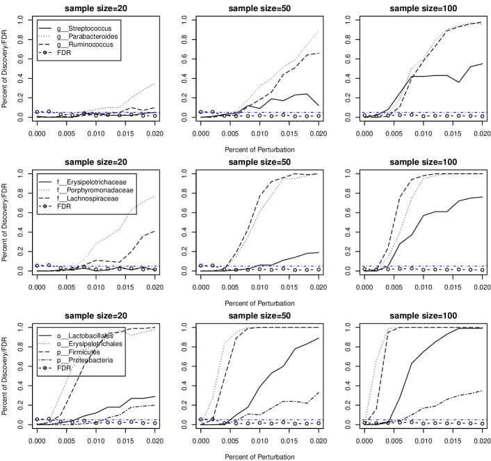
(b) Dense differential pattern setting.

Figure 4: Identification of subtrees with differential subcompositions with FDR set to 0.05. y-axis shows the percent of discovery of the corresponding subtree in 100 simulations with FDR controlled at 0.05. The empirical FDR is close to 0.05. In this series of figures, only some of the subtrees with parent node that has detectable differential subcompositions are shown. In figure legend, g_, f_, o_, p_ represent genus, family, order and phylum, respectively.

6 Analysis of Microbiome Data in the Upper Respiratory Tract

The human nasopharynx and oropharynx are two body sites located very close to each other in the upper respiratory tract. The nasopharynx is the ecological niche for many commensal bacteria. It is interesting to understand whether these nearby sites have similar microbiome composition and how smoking perturbs their compositions. Charlson et al. (2010) collected the left and right nasopharynx and oropharynx microbiome samples from 32 current smokers and 36 nonsmokers. The samples were sequenced using 16S rRNA sequencing, and the count of reads are aligned onto a taxonomic tree with 213 nodes from kingdom to species. One nonsmoker and one smoker had missing left nasopharynx sample, and one smoker had missing right oropharynx sample.

Several comparisons of the overall microbiome compositions were compared and the results are summarized in Table 1. As expected, no significant differences were observed between left and right nasopharynx or oropharynx. However very significant differences were observed between nasopharynx and oropharynx both in the left and right sides, further confirming the niche-specific colonization at discrete anatomical sites. In addition, smoking had strong effects on microbiome composition in both nasopharynx and oropharynx

Table 1: $p-$values of different comparisons between two body sites and between smokers and non-smokers based on the proposed tests using the Fisher’s method or the 2nd smallest p value and PERMANOVA.

	PairMN (Fisher $||$ 2nd)	PERMANOVA
Nasopharynx and Oropharynx (Left Side)	0 $||$ 0	$<$0.001
Nasopharynx and Oropharynx (Right Side)	0 $||$ 0	$<$0.001
Smoker vs Nonsmoker (nasopharynx)	2.1e-07 $||$ 8.6e-05	0.003
Smoker vs Nonsmoker (oropharynx )	1.2e-07 $||$ 6.2e-04	0.005
Left vs Right (nasopharynx)	0.16 $||$ 0.65	0.053
Left vs Right (oropharynx )	0.37 $||$ 0.79	0.99

6.1 Comparison of nasopharynx and oropharynx microbiome for nonsmokers

Since a large overall microbiome composition difference was observed, it is interesting to identify which subtrees and their corresponding subcompositions led to such a difference. The proposed subtree identification procedure in Section 4.3 using the pairNM test in (11) was applied to identify the subtrees with differential subcompositions between the two body sites at an FDR=0.05. The identified parental nodes, their child nodes and the corresponding subcompositions are shown in Figure 5 (a). One advantage of the proposed method is to identify these subtrees at various taxonomic levels. For example, at the phylum level, nasopharynx clearly had more Firmicutes, however, oropharynx had more Bacteroidetes. At the genus level, Streptococcus appeared more frequently in oropharynx, but Lactococcus occurred more in nasopharynx.

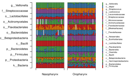
(a) Comparison between left nasopharynx and left oropharynx among nonsmokers.

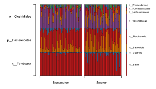
(b) Comparison between smokers and nonsmokers in nasopharynx.

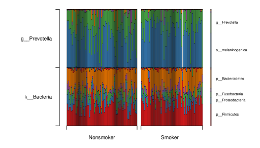
(c) Comparison between smokers and nonsmokers in oropharynx.

Figure 5: Analysis of upper respiratory tract microbiome data. Parental nodes and the child nodes that showed differential subcomposition are presented. In taxon labels, g_, f_, o_, p_ represent genus, family, order and phylum, respectively. For (a), the sample size is 35. The number of parameters within each subtree ranges from 2 to 6. For (b), the sample size is 71 for nonsmokers and 63 for smokers. The number of parameters to test within each subtree ranges from 2 to 6. For (c), the sample size is 72 for nonsmokers and 63 for smokers. The number of parameters to test within each subtree ranges from 2 to 10.

6.2 Comparison of microbiome between smokers and non-smokers

The proposed procedure was also applied to identify the differential subtrees with differential subcompositions between smokers and nonsmokers in nasopharynx and oropharynx and the results are shown in Figures 5 (b) and (c) for an FDR=0.05. For nasopharynx, the subcompositions of classes under Phylum Firmicutes, classes under Phylum Bacteroidetes and families under Order Clostridiale were different, with fewer Bacilli in Firmicutes, more Bacteroidia in Bacteroidetes, and fewer Veillonellaceae in Clostridiales being observed in smokers (Figure 5 (b)).

For oropharynx, differences in the subcomposition of phyla and species under Genus Prevotalla were observed, with more Firmicuates in Kingdom Bacteria and more Melaninogenica in Genus Prevotella observed in smokers (Figure 5 (c)).

7 Discussion

This paper has introduced a flexible model for paired multinomial data. Based on this model, a $T^{2}$-type of test statistic has been developed for testing equality of the overall taxa composition between two repeatedly measured multinomial data. The test can be used for analysis of count data observed on a taxonomic tree to identify the subtrees that show differential subcompositions in repeated measures. Our simulations have shown that the proposed test has correct type 1 errors and much increased power than the commonly used tests based on DM model or the PERMANOVA test. The test proposed in this paper can be applied to both independent and repeated measurement data. For independent data, the proposed test allows more flexible dependency structure among the taxa than the Dirichlet-multinomial model, which only allows negative correlations among the taxa. The proposed test statistics are also computationally more efficient than the commonly used permutation-based procedures such as PERMANOVA, which enables their applications in large-scale microbiome studies.

As demonstrated in our simulations, the proposed overall test of composition is more powerful than PERMANOVA type of tests when the overall composition difference is due to a few subcompositions since our test considers each subtree and subcomposition separately and then combines the $p$-values. Since the tests for differential subcomposition condition on the total counts of the parental nodes, all the $p$-values are independent, which facilitates simple combination of $p$-values and identification of the subtrees based on FDR controlling. In general, test based on the $2^{nd}$ smallest $p$-value for overall composition difference is more sensitive than the Fisher’s method, as is shown in simulations in Section 5.2. However, the Fisher’s method is expected to have higher power when most of the subtrees show differential compositions. When the differential pattern is not known, one possible solution is to take the smallest of these two $p$-values and to use permutations to assess its significance.

Although the paper has focused on using existing taxonomic tree and 16S sequencing data, the tests proposed in this paper can also be applied to shotgun metagenomic sequencing data. One possible approach is to build phylogenetic trees based on a small set of universal marker genes (Sunagawa et al., 2013) and to align the sequencing reads to these phylogenetic trees. The proposed methods can be applied to each of these trees and the results can be combined. This deserves further investigation.

Appendix - Proofs

Proof of Lemma 1

By (6), we have

$$\text{Var}\hat{\boldsymbol{\pi}}_{t} = \dfrac{\sum_{i=1}^{n}N_{it}^{2}-N_{\cdot t}}{N_{\cdot t}^{2}}\boldsymbol{\Sigma}_{t}+\dfrac{1}{N_{\cdot t}}\big{(}diag(\boldsymbol{\pi}_{t})-\boldsymbol{\pi}_{t}\boldsymbol{\pi}_{t}^{\top}\big{)},$$

$$\text{Cov}(\hat{\boldsymbol{\pi}}_{1},\hat{\boldsymbol{\pi}}_{2}) = \dfrac{\sum_{i=1}^{n}N_{i1}N_{i2}}{N_{\cdot 1}N_{\cdot 2}}\boldsymbol{\Sigma}_{12}.$$

It can also be shown that

$$\mathbb{E}(\mathbf{S}_{t}-\mathbf{G}_{t}) = N_{ct}\boldsymbol{\Sigma}_{t},$$

$$\mathbb{E}\big{(}\mathbf{S}_{t}+(N_{ct}-1)\mathbf{G}_{t}\big{)} = N_{ct}\big{(}diag(\boldsymbol{\pi}_{t})-\boldsymbol{\pi}_{t}\boldsymbol{\pi}_{t}^{\top}\big{)},$$

$$\mathbb{E}\widehat{\boldsymbol{\Sigma}}_{12} = \boldsymbol{\Sigma}_{12}.$$

Thus,

$$\begin{split}\boldsymbol{\Sigma}_{\hat{\pi}}~{}=~{}&\text{Var}(\hat{\boldsymbol{\pi}}_{1}-\hat{\boldsymbol{\pi}}_{2})\\ ~{}=~{}&\sum_{t=1}^{2}\left\{\dfrac{\sum_{i=1}^{n}N_{it}^{2}-N_{\cdot t}}{N_{\cdot t}^{2}}\boldsymbol{\Sigma}_{t}+\dfrac{1}{N_{\cdot t}}\big{(}diag(\boldsymbol{\pi}_{t})-\boldsymbol{\pi}_{t}\boldsymbol{\pi}_{t}^{\top}\big{)}\right\}-\dfrac{2\sum_{i=1}^{n}N_{i1}N_{i2}}{N_{\cdot 1}N_{\cdot 2}}\boldsymbol{\Sigma}_{12}\\ ~{}=~{}&\sum_{t=1}^{2}\left\{\dfrac{\sum_{i=1}^{n}N_{it}^{2}-N_{\cdot t}}{N_{ct}N_{\cdot t}^{2}}\mathbb{E}(\mathbf{S}_{t}-\mathbf{G}_{t})+\dfrac{1}{N_{ct}N_{\cdot t}}\mathbb{E}\big{(}\mathbf{S}_{t}+(N_{ct}-1)\mathbf{G}_{t}\big{)}\right\}\\ &~{}-~{}\dfrac{\sum_{i=1}^{n}N_{i1}N_{i2}}{N_{\cdot 1}N_{\cdot 2}}\mathbb{E}\big{(}\widehat{\boldsymbol{\Sigma}}_{12}+\widehat{\boldsymbol{\Sigma}}_{12}^{\top}\big{)}.\end{split}$$ (23)

By law of large numbers, the following convergences hold in probability as $n\rightarrow\infty$.

$$\begin{split}||(\mathbf{S}_{t}-\mathbf{G}_{t})-\mathbb{E}(\mathbf{S}_{t}-\mathbf{G}_{t})||_{\max}~{}\rightarrow~{}&0,\\ ||\big{(}\mathbf{S}_{t}+(N_{ct}-1)\mathbf{G}_{t}\big{)}-\mathbb{E}\big{(}\mathbf{S}_{t}+(N_{ct}-1)\mathbf{G}_{t}\big{)}||_{\max}~{}\rightarrow~{}&0,\\ ||\boldsymbol{\Sigma}_{12}-\mathbb{E}\widehat{\boldsymbol{\Sigma}}_{12}||_{\max}~{}\rightarrow~{}&0.\end{split}$$ (24)

Combining (8), (23) and (24), we have

$$||\widehat{\boldsymbol{\Sigma}}_{\hat{\pi}}-\boldsymbol{\Sigma}_{\hat{\pi}}||_{\max}\rightarrow 0\quad\mbox{ in probability as }n\rightarrow\infty$$

Proof of Theorem 1

Define $S^{d-1}=\{x\in\mathbb{R}^{p}:\boldsymbol{1}^{\top}x=0\}$. Then $\boldsymbol{\pi}_{1}-\boldsymbol{\pi}_{2},\hat{\boldsymbol{\pi}}_{1}-\hat{\boldsymbol{\pi}}_{2}\in S^{d-1}$. Therefore

$$(\hat{\boldsymbol{\pi}}_{1}-\hat{\boldsymbol{\pi}}_{2})^{\top}\boldsymbol{\Sigma}_{\hat{\pi}}^{\dagger}(\hat{\boldsymbol{\pi}}_{1}-\hat{\boldsymbol{\pi}}_{2})\rightarrow\chi_{d-1}^{2}.$$

We show next that $\widehat{\boldsymbol{\Sigma}}_{\hat{\pi}}^{\dagger}\rightarrow\boldsymbol{\Sigma}_{\hat{\pi}}^{\dagger}$ in probability. Then by Slutsky Theorem, for fixed $d$ and $n\rightarrow\infty$,

$$F=\dfrac{n-d+1}{(n-1)(d-1)}(\hat{\boldsymbol{\pi}}_{1}-\hat{\boldsymbol{\pi}}_{2})^{\top}\widehat{\boldsymbol{\Sigma}}_{\hat{\pi}}^{\dagger}(\hat{\boldsymbol{\pi}}_{1}-\hat{\boldsymbol{\pi}}_{2})\rightarrow\chi_{d-1}^{2}/(d-1)$$

Since $F_{d-1,n-d+1}\rightarrow\chi^{2}_{d-1}/(d-1)$ for fixed $d$ and $n\rightarrow\infty$, $F>F_{d-1,n-d+1}^{-1}(1-\alpha)$ is an asymptotic level $\alpha$ test.

Let $\boldsymbol{\Gamma}$ be an orthogonal matrix in the form of $[\mathbf{V},\boldsymbol{1}^{\top}_{d}/\sqrt{d}]$. Then, because $\boldsymbol{1}_{d}^{\top}\widehat{\boldsymbol{\Sigma}}_{\hat{\pi}}=\boldsymbol{1}_{d}^{\top}\boldsymbol{\Sigma}_{\hat{\pi}}=0$, by Lemma 1, we have

$$\begin{split}||\mathbf{V}^{\top}(\widehat{\boldsymbol{\Sigma}}_{\hat{\pi}}-\boldsymbol{\Sigma}_{\hat{\pi}})\mathbf{V}||_{2}/d\leq||\mathbf{V}^{\top}(\widehat{\boldsymbol{\Sigma}}_{\hat{\pi}}-\boldsymbol{\Sigma}_{\hat{\pi}})\mathbf{V}||_{\max}=||\mathbf{\Gamma}^{\top}(\widehat{\boldsymbol{\Sigma}}_{\hat{\pi}}-\boldsymbol{\Sigma}_{\hat{\pi}})\mathbf{\Gamma}||_{\max}\rightarrow 0\quad\mbox{in probability}\end{split}$$

where $||\cdot||_{2}$ is the spectral norm of matrix. Define $\boldsymbol{\Delta}=\mathbf{V}^{\top}(\widehat{\boldsymbol{\Sigma}}_{\hat{\pi}}-\boldsymbol{\Sigma}_{\hat{\pi}})\mathbf{V}$. Using Neumann series expansion,

$$\begin{split}(\mathbf{V}^{\top}\widehat{\boldsymbol{\Sigma}}_{\hat{\pi}}\mathbf{V})^{-1}-(\mathbf{V}^{\top}\boldsymbol{\Sigma}_{\hat{\pi}}\mathbf{V})^{-1}&=(\mathbf{V}^{\top}\boldsymbol{\Sigma}_{\hat{\pi}}\mathbf{V})^{-1}\sum_{i=1}^{\infty}\big{(}-(\mathbf{V}^{\top}\boldsymbol{\Sigma}_{\hat{\pi}}\mathbf{V})\boldsymbol{\Delta}\big{)}^{i},\end{split}$$

therefore,

$$||(\mathbf{V}^{\top}\widehat{\boldsymbol{\Sigma}}_{\hat{\pi}}\mathbf{V})^{-1}-(\mathbf{V}^{\top}\boldsymbol{\Sigma}_{\hat{\pi}}\mathbf{V})^{-1}||_{2}\leq\sum_{i=0}^{\infty}||\mathbf{V}^{\top}\boldsymbol{\Sigma}_{\hat{\pi}}\mathbf{V}||_{2}^{i}||\boldsymbol{\Delta}||_{2}^{i+1}.$$

Because $||\mathbf{V}^{\top}\boldsymbol{\Sigma}_{\hat{\pi}}\mathbf{V}||_{2}$ is fixed, we have $||\mathbf{V}^{\top}\boldsymbol{\Sigma}_{\hat{\pi}}\mathbf{V}||_{2}||\boldsymbol{\Delta}||_{2}\rightarrow 0$ in probability, which implies $\mathbb{P}\big{(}||\mathbf{V}^{\top}\boldsymbol{\Sigma}_{\hat{\pi}}\mathbf{V}||_{2}||\boldsymbol{\Delta}||_{2}<1\big{)}\rightarrow 1.$ Therefore, with probability one,

$$\sum_{i=0}^{\infty}||\mathbf{V}^{\top}\boldsymbol{\Sigma}_{\hat{\pi}}\mathbf{V}||_{2}^{i}||\boldsymbol{\Delta}||_{2}^{i+1}=\dfrac{||\boldsymbol{\Delta}||_{2}}{1-||\mathbf{V}^{\top}\boldsymbol{\Sigma}_{\hat{\pi}}\mathbf{V}||_{2}||\boldsymbol{\Delta}||_{2}}$$

holds. As a result,

$$\begin{split}||(\mathbf{V}^{\top}\widehat{\boldsymbol{\Sigma}}_{\hat{\pi}}\mathbf{V})^{-1}-(\mathbf{V}^{\top}\boldsymbol{\Sigma}_{\hat{\pi}}\mathbf{V})^{-1}||_{\max}&\leq||(\mathbf{V}^{\top}\widehat{\boldsymbol{\Sigma}}_{\hat{\pi}}\mathbf{V})^{-1}-(\mathbf{V}^{\top}\boldsymbol{\Sigma}_{\hat{\pi}}\mathbf{V})^{-1}||_{2}\\ &\leq\dfrac{||\boldsymbol{\Delta}||_{2}}{1-||\mathbf{V}^{\top}\boldsymbol{\Sigma}_{\hat{\pi}}\mathbf{V}||_{2}||\boldsymbol{\Delta}||_{2}}\rightarrow 0\quad\mbox{in probability},\end{split}$$

which leads to

$$||\mathbf{V}(\mathbf{V}^{\top}\widehat{\boldsymbol{\Sigma}}_{\hat{\pi}}\mathbf{V})^{-1}\mathbf{V}^{\top}-\mathbf{V}(\mathbf{V}^{\top}\boldsymbol{\Sigma}_{\hat{\pi}}\mathbf{V})^{-1}\mathbf{V}^{\top}||_{\max}\rightarrow 0\quad\mbox{in probability}.$$ (25)

Suppose we have the eigenvalue decomposition of $\boldsymbol{\Sigma}_{\hat{\pi}}$ as $\boldsymbol{\Sigma}_{\hat{\pi}}=\mathbf{U}\boldsymbol{\Lambda}\mathbf{U}^{\top}$, where $\mathbf{U}\in\mathbb{R}^{d\times(d-1)}$ and $\boldsymbol{\Lambda}\in\mathbb{R}^{(d-1)\times(d-1)}$. Then $\boldsymbol{1}_{d}^{\top}\mathbf{U}=0$. Also, $\mathbf{U}^{\top}\mathbf{V}$ is orthogonal because

$$\mathbf{U}^{\top}\mathbf{V}\mathbf{V}^{\top}\mathbf{U}=\mathbf{U}^{\top}(\textbf{I}_{d}-\boldsymbol{1}_{d}\boldsymbol{1}_{d}^{\top}/d)\mathbf{U}=\mathbf{U}^{\top}\mathbf{U}=\textbf{I}_{d-1}$$

Therefore,

$$\begin{split}&\mathbf{V}(\mathbf{V}^{\top}\boldsymbol{\Sigma}_{\hat{\pi}}\mathbf{V})^{-1}\mathbf{V}^{\top}=\mathbf{V}(\mathbf{V}^{\top}\mathbf{U}\boldsymbol{\Lambda}\mathbf{U}^{\top}\mathbf{V})^{-1}\mathbf{V}^{\top}\\ &=\mathbf{V}(\mathbf{U}^{\top}\mathbf{V})^{-1}\boldsymbol{\Lambda}^{-1}(\mathbf{V}^{\top}\mathbf{U})^{-1}\mathbf{V}^{\top}=\mathbf{V}(\mathbf{U}^{\top}\mathbf{V})^{\top}\boldsymbol{\Lambda}^{-1}(\mathbf{V}^{\top}\mathbf{U})^{\top}\mathbf{V}^{\top}\\ &=(\textbf{I}_{d}-\boldsymbol{1}_{d}\boldsymbol{1}_{d}^{\top}/d)\mathbf{U}\boldsymbol{\Lambda}^{-1}\mathbf{U}^{\top}(\textbf{I}_{d}-\boldsymbol{1}_{d}\boldsymbol{1}_{d}^{\top}/d)=\mathbf{U}\boldsymbol{\Lambda}^{-1}\mathbf{U}^{\top}\\ &=\boldsymbol{\Sigma}_{\hat{\pi}}^{\dagger}.\end{split}$$

Similarly, we have

$$\widehat{\boldsymbol{\Sigma}}_{\hat{\pi}}^{\dagger}=\mathbf{V}(\mathbf{V}^{\top}\widehat{\boldsymbol{\Sigma}}_{\hat{\pi}}\mathbf{V})^{-1}\mathbf{V}^{\top}.$$

The proof of this statement is similar to the proof of $\boldsymbol{\Sigma}_{\hat{\pi}}^{\dagger}=\mathbf{V}(\mathbf{V}^{\top}\boldsymbol{\Sigma}_{\hat{\pi}}\mathbf{V})^{-1}\mathbf{V}^{\top}$. Because $n>d$, we still have the eigenvalue decomposition of $\widehat{\boldsymbol{\Sigma}}_{\hat{\pi}}$ as $\widehat{\boldsymbol{\Sigma}}_{\hat{\pi}}=\mathbf{U}\boldsymbol{\Lambda}\mathbf{U}^{\top}$, where $\mathbf{U}\in\mathbb{R}^{d\times(d-1)}$ and $\boldsymbol{\Lambda}\in\mathbb{R}^{(d-1)\times(d-1)}$. Then $\boldsymbol{1}_{d}^{\top}\mathbf{U}=0$. Also, $\mathbf{U}^{\top}\mathbf{V}\in\mathbb{R}^{(d-1)\times(d-1)}$ is orthogonal because $\mathbf{U}^{\top}\mathbf{V}\mathbf{V}^{\top}\mathbf{U}=\mathbf{U}^{\top}(\textbf{I}_{d}-\boldsymbol{1}_{d}\boldsymbol{1}_{d}^{\top}/d)\mathbf{U}=\mathbf{U}^{\top}\mathbf{U}=\textbf{I}_{d-1}.$

Further, we show that $\widehat{\boldsymbol{\Sigma}}_{\hat{\pi}}^{\dagger}$ is indeed a generalized inverse of $\widehat{\boldsymbol{\Sigma}}_{\hat{\pi}}$, because

$$\begin{split}\widehat{\boldsymbol{\Sigma}}_{\hat{\pi}}^{\dagger}\widehat{\boldsymbol{\Sigma}}_{\hat{\pi}}\widehat{\boldsymbol{\Sigma}}_{\hat{\pi}}^{\dagger}&=\mathbf{V}(\mathbf{V}^{\top}\mathbf{U}\mathbf{\Lambda}\mathbf{U}^{\top}\mathbf{V})^{-1}\mathbf{V}^{\top}\mathbf{U}\mathbf{\Lambda}\mathbf{U}^{\top}\mathbf{V}(\mathbf{V}^{\top}\mathbf{U}\mathbf{\Lambda}\mathbf{U}^{\top}\mathbf{V})^{-1}\mathbf{V}^{\top}\\ &=\mathbf{V}(\mathbf{U}^{\top}\mathbf{V})^{-1}\mathbf{\Lambda}^{-1}(\mathbf{V}^{\top}\mathbf{U})^{-1}\mathbf{V}^{\top}\mathbf{U}\mathbf{\Lambda}\mathbf{U}^{\top}\mathbf{V}(\mathbf{U}^{\top}\mathbf{V})^{-1}\mathbf{\Lambda}^{-1}(\mathbf{V}^{\top}\mathbf{U})^{-1}\mathbf{V}^{\top}\\ &=\mathbf{V}(\mathbf{U}^{\top}\mathbf{V})^{-1}\mathbf{\Lambda}^{-1}(\mathbf{V}^{\top}\mathbf{U})^{-1}\mathbf{V}^{\top}\\ &=\mathbf{V}(\mathbf{U}^{\top}\mathbf{V})^{\top}\mathbf{\Lambda}^{-1}(\mathbf{V}^{\top}\mathbf{U})^{\top}\mathbf{V}^{\top}=(\mathbf{V}\mathbf{V}^{\top})\mathbf{U}\mathbf{\Lambda}^{-1}\mathbf{U}^{\top}(\mathbf{V}\mathbf{V}^{\top})\\ &=(\textbf{I}_{d}-\textbf{1}_{d}\textbf{1}_{d}/d)\mathbf{U}\mathbf{\Lambda}^{-1}\mathbf{U}^{\top}(\textbf{I}_{d}-\textbf{1}_{d}\textbf{1}_{d}/d)\\ &=\mathbf{U}\mathbf{\Lambda}^{-1}\mathbf{U}^{\top}=\widehat{\boldsymbol{\Sigma}}_{\hat{\pi}}^{\dagger}.\end{split}$$

Based on (25), we have

$$||\widehat{\boldsymbol{\Sigma}}_{\hat{\pi}}^{\dagger}-\boldsymbol{\Sigma}_{\hat{\pi}}^{\dagger}||_{\max}\rightarrow 0\mbox{ in probability}.$$

References

- Altschul et al. (1990) Altschul, S., Gish, W., Miller, W., Myers, E., and Lipman, D. (1990). Basic local alignment search tool. Journal of Molecular Biology, 215:403–401.
- Anderson (2001) Anderson, M. J. (2001). A new method for non-parametric multivariate analysis of variance. Austral Ecology, 26:32–46.
- Asnicar et al. (2015) Asnicar, F., Weingart, G., Tickle, T., Huttenhower, C., and Segata, N. (2015). Compact graphical representation of phylogenetic data and metadata with graphlan. PeerJ, 3:e1029.
- Benjamini and Hochberg (1995) Benjamini, Y. and Hochberg, Y. (1995). Controlling the false discovery rate: a practical and powerful approach to multiple testing. J. R. Statis. Soc. B, 57:289–300.
- Charlson et al. (2010) Charlson, E., Chen, J., Custers-Allen, R., Bittinger, K., Li, H., Sinha, R., Hwang, J., Bushman, F., and Collman, R. (2010). Disordered microbial communities in the upper respiratory tract of cigarette smokers. PloS one, 5:e15216.
- Chen and Li (2013) Chen, J. and Li, H. (2013). Variable selection for sparse dirichlet-multinomial regression with an application to microbiome data analysis. Annals of Applied Statistics, 7:418–442.
- Clarke (1993) Clarke, K. (1993). Non-parametric multivariate analysis of changes in community structure. Australian Journal of Ecology, 18:117–143.
- Cole et al. (2007) Cole, J., Chai, B., Farris, R., Wang, Q., Kulam-Syed-Mohideen, A., McGarrell, D., Bandela, A., Cardenas, E., Garrity, G., and Tiedje, J. (2007). The ribosomal database project (rdp-ii): introducing myrdp space and quality controlled public data. Nucleic Acids Res., 35:D169–D172.
- DeSantis et al. (2006) DeSantis, T., Hugenholtz, P., Larsen, N., Rojas, M., Brodie, E., Keller, K., Huber, T., Dalevi, D., Hu, P., and Andersen, G. (2006). Greengenes, a chimera-checked 16s rrna gene database and workbench compatible with arb. Applied Environmental Microbiology, 72:5059–5072.
- Evans and Matsen (2012) Evans, S. N. and Matsen, F. A. (2012). The phylogenetic kantorovich-rubinstein metric for environmental sequence samples. J. R. Statist. Soc. B, 74:569–592.
- Flores et al. (2014) Flores, G., Caporaso, J., Henley, J., Rideout, J., Domogala, D., Chase, J., Leff, J., Vázquez-Baeza, Y., Gonzalez, A., Knight, R., Dunn, R., and Fierer, N. (2014). Temporal variability is a personalized feature of the human microbiome. Genome Biology, 15:531.
- Gill et al. (2006) Gill, S., Pop, M., DeBoy, R., Eckburg, P., Turnbaugh, P., Samuel, B., Gordon, J., Relman, D., Fraser-Liggett, C., and Nelson, K. (2006). Metagenomic analysis of the human distal gut microbiome. Science, 312(5778):1355–1359.
- La Rosa et al. (2012) La Rosa, P. S., Brooks, J. P., Deych, E., L., B. E., Edwards, D. J., Wang, Q., Sodergren, E., Weinstock, G., and Shannon, W. D. (2012). Hypothesis testing and power calculations for taxonomic-based human microbiome data. PLoS ONE, 7:e52078.
- Liu et al. (2008) Liu, J., DeSantis, T., Anderson, G., and Knight, R. (2008). Accurate taxonomy assignments from 16s rrna sequences produced by highly parallel pyrosequencers. Nucleic Acids Research, 36:e120.
- Mandal et al. (2015) Mandal, S., Van Treuren, W., White, R., Eggesbo, M., Knight, R., and Peddada, S. (2015). Analysis of composition of microbiomes: a novel method for studying microbial composition. Microbial Ecology in Health and Disease, 26:27663.
- Manichanh et al. (2012) Manichanh, C., Borruel, N., Casellas, F., and Guarner, F. (2012). The gut microbiota in ibd. Nature Reviews Gastroenterology and Hepatology, 9(10):599–608.
- Mantel (1967) Mantel, N. (1967). The detection of disease clustering and a generalized regression approach. Cancer Research, 27:209–220.
- Qin et al. (2010) Qin, J., Li, R., Raes, J., Arumugam, M., Burgdorf, K., Manichanh, C., Nielsen, T., Pons, N., Levenez, F., Yamada, T., et al. (2010). A human gut microbial gene catalogue established by metagenomic sequencing. Nature, 464(7285):59–65.
- Qin et al. (2012) Qin, J., Li, Y., Cai, Z., Li, S., Zhu, J., Zhang, F., Liang, S., Zhang, W., Guan, Y., Shen, D., et al. (2012). A metagenome-wide association study of gut microbiota in type 2 diabetes. Nature, 490(7418):55–60.
- Sunagawa et al. (2013) Sunagawa, S., Mende, D., Zeller, G., Izquierdo-Carrasco, F., Berger, S., Kultima, J., Coelho, L., Arumugam, M., Tap, J., Nielsen, H., Rasmussen, S., Brunak, S., Pedersen, O., Guarner, F., de Vos, W., Wang, J., Li, J., Doré, J., Ehrlich, S., Stamatakis, A., and Bork, P. (2013). Metagenomic species profiling using universal phylogenetic marker genes. Nature Methods, 10:1196–1199.
- Turnbaugh et al. (2007) Turnbaugh, P., Ley, R., Hamady, M., Fraser-Liggett, C., Knight, R., and Gordon, J. (2007). The human microbiome project. Nature, 449(7164):804–810.
- Turnbaugh et al. (2006) Turnbaugh, P., Ley, R., Mahowald, M., Magrini, V., Mardis, E., and Gordon, J. (2006). An obesity-associated gut microbiome with increased capacity for energy harvest. Nature, 444(7122):1027–131.
- Wilkinson (1951) Wilkinson, B. (1951). A statistical consideration in psychological research. Psychological bulletin, 48(2):156.
- Wilson (1989) Wilson, J. R. (1989). Chi-square tests for overdispersion with multiparameter estimates. J. R. Statist. Soc. C, 38:441–453.
- Zaykin et al. (2002) Zaykin, D. V., Zhivotovsky, L. A., Westfall, P. H., and Weir, B. S. (2002). Truncated product method for combining p-values. Genetic epidemiology, 22(2):170–185.