Analysis of Tsallis’ classical partition function’s poles

Abstract

When one integrates the q-exponential function of Tsallis’ so as to get the partition function $Z$, a gamma function inevitably emerges. Consequently, poles arise. We investigate here here the thermodynamic significance of these poles in the case of $n$ classical harmonic oscillators (HO). Given that this is an exceedingly well known system, any new feature that may arise can safely be attributed to the poles’ effect. We appeal to the mathematical tools used in [EPJB 89, 150 (2016) and ArXiv:1702.03535 (2017)], and obtain both bound and unbound states. In the first case, we are then faced with a classical Einstein crystal. We also detect what might be interpreted as pseudo gravitational effects.

Keywords: q-Statistics, divergences, partition function, dimensional regularization, specific heat.

1 Introduction

Tsallis’ q-statistical mechanics yielded variegated applications in the last 25 years [1, 2, 3, 4, 5, 6, 7, 8, 9, 10, 11, 12]. This statistics is of great importance for astrophysics, in what respects to self-gravitating systems [13, 14, 15]. Further, it was shown to be useful in diverse scientific fields. It has to its credit several thousands of papers and authors [2]. Investigating its structural characteristics should be important for astronomy, physics, neurology, biology, economic sciences, etc. [1]. Paradigmatic example is found in its application to high energy physics, where the q-statistics seems to describe well the transverse momentum distributions of different hadrons [16, 17, 18].

In this work we use standard mathematical tools described in [19, 20] to investigate interesting properties of the Tsallis statistics of n harmonic oscillators.

The central point is the fact that the integrals used to evaluate the partition function $Z$ and the mean energy $<U>$ diverge for specific q-values. These divergences can be overcome as described in [19, 20]

A basic result to be obtained here is that the number of classical oscillators, $n$, is strongly limited by the dimensionality $\nu$ and the Tsallis parameter q. For $<U>>0$ and $Z>0$, i.e., the conventional theory, $n$ must be finite and bounded.

A different panorama emerges by recourse to analytical extension in $\nu$. Then it is possible to have a situation in which $Z>0$, $<U><0$, $C<0$, with n finite and bounded. Thus, our systems are here bound, representing a ”classical crystal”, and also self-gravitating [15]. Finally, we will study the theory’s poles by recourse to dimensional regularization [19, 20]. We find at the poles, that i) the specific heat $C$ is temperature ($T$) dependent (classically!), and, ii) again, gravitational effects. Note the $C$ can be $T-$dependent only due to internal degrees of freedom, and that this is a quantum effect. We detect this dependence here at a purely classical level.

We are motivated by the need of trying to determine what kind of hidden correlations are entailed by the non additivity of Tsallis’ entropy $S_{q}$ for two independent systems A, B, i.e.,

$$S_{q}(A,B)=S_{q}(A)+S_{q}(B)+(1-q)S_{q}(A)S:q(B);\,\,\,q\in{\cal R}.$$

This is conveniently done by appeal to quite simple systems, whose physics is well known. Any divergence from this physics will originate in the hidden correlations. This is why we employ a system of $n$ HOs here.

Divergences constitute an important theme of theoretical physics. The study and elimination of these divergences may be one of the most relevant tasks of theoretical endeavor. The typical example is the (thus far failed, alas) attempt to quantify the gravitational field. Examples of divergences-elimination can be found in references [21, 22, 23, 24, 25].

We use here an quite simplified version (see [26]), of the methodology of [21, 22, 23, 24, 25] with regards to Tsallis statistics [1, 2], focusing on its applicability to self-gravitation [13, 14, 15]. Divergence’s removal will be seen to yield quite interesting insights.

These emerge using mathematics well known for the last 40 years ago. Their development allowed M. Veltman and G. t’Hooft to be awarded with the Nobel prize of physics in 1999. Comfortable acquaintance with these mathematics is not a prerequisite to follow this paper. However, one must accept that their physical significance is not now to kin doubt. In fact, one just needs i) analytical extensions and ii) dimensional regularization [21, 22, 23, 24, 25].

We will here analyze the behavior of $Z$ and $<U>$ in connection with three zones of possible arguments of the $\Gamma$-function thay appears in $Z$ and $<U>$. These arguments of the $\Gamma$-function rule the $Z$ - $<U>$ behavior, that in turn produces three distinct zones, for a given spatial dimension $\nu$, Tsallis’ index $q$ and number of particles $N$. The zone’s specifics are:
$(1)\;\;\;\frac{1}{1-q}-n\nu-1>0$
$(2)\;\;\;\frac{1}{1-q}-n\nu<0\;\;\;\Gamma\left(\frac{1}{1-q}-n\nu\right)>0$
$(3)\;\;\;\frac{1}{1-q}-n\nu=-p\;\;\;p=0,1,2,3,4.....$
Normal behavior is found in zone (1). Something resembling what might constitute gravitational effects (GE) are encountered in zone (2). In zone (3) we find both normal behavior and also GE (Also known as gravotermal effects).

Remark than in instance (3) we are performing a regularization of the corresponding theory, not a renormalization.

2 The Harmonic Oscillator

It has to be noted, from the beginning, that we use in this contribution normal (linear in the probability) expectation values. For simplicity reasons, we do not appeal to the weighted ones, customarily attached to Tsallis-related papers [1]. In this case one restricts oneself to the interval $[0<q\leq 1]$, and, consequently, the so-called Tsallis cut-off problem [1] is avoided.

For the q-partition function one has

$$Z=V^{n}\int\limits_{-\infty}^{\infty}\left[1+\beta(1-q)(p_{1}^{2}+\cdot\cdot\cdot p_{n}^{2}+q_{1}^{2}+\cdot\cdot\cdot q_{n}^{2})\right]^{\frac{1}{q-1}}\otimes$$

$$d^{\nu}p_{1}\cdot\cdot\cdot d^{\nu}p_{n}d^{\nu}q_{1}\cdot\cdot\cdot d^{\nu}q_{n},$$ (2.1)

Or

$$Z=\frac{2\pi^{\nu n}}{\Gamma\left(\nu n\right)}\int\limits_{-\infty}^{\infty}\left[1+\beta(1-q)p^{2}\right]^{\frac{1}{q-1}}p^{2\nu n-1}dp.$$ (2.2)

We have integrated over the angles and taken $p^{2}=p_{1}^{2}+\cdot\cdot\cdot p_{n}^{2}+q_{1}^{2}+\cdot\cdot\cdot q_{n}^{2}$. Changing variables in the fashion $x=p^{2}$, the last integral becomes

$$Z=\frac{\pi^{\nu n}}{\Gamma\left(\nu n\right)}\int\limits_{-\infty}^{\infty}\left[1+\beta(1-q)x\right]^{\frac{1}{q-1}}x^{\nu n-1}dx,$$ (2.3)

that evaluated, yields

$$Z=\left[\frac{\pi}{\beta(1-q)}\right]^{\nu n}\frac{\Gamma\left(\frac{1}{1-q}-\nu n\right)}{\Gamma\left(\frac{1}{1-q}\right)}.$$ (2.4)

Similarly we have

$$Z<U>=\int\limits_{-\infty}^{\infty}\left[1+\beta(1-q)(p_{1}^{2}+\cdot\cdot\cdot p_{n}^{2}+q_{1}^{2}+\cdot\cdot\cdot q_{n}^{2})\right]^{\frac{1}{q-1}}$$

$$(p_{1}^{2}+\cdot\cdot\cdot p_{n}^{2}+q_{1}^{2}+\cdot\cdot\cdot q_{n}^{2})d^{\nu}p_{1}\cdot\cdot\cdot d^{\nu}q_{n}.$$ (2.5)

In spherical coordinates this becomes

$$Z<U>=\frac{2\pi^{\nu n}}{\Gamma\left(\frac{\nu n}{2}\right)}\int\limits_{-\infty}^{\infty}\left[1+\beta(1-q)p^{2}\right]^{\frac{1}{q-1}}p^{2\nu n+1}dp,$$ (2.6)

and setting $x=p^{2}$ this is now

$$Z<U>=\frac{\pi^{\nu n}}{\Gamma\left(\nu n\right)}\int\limits_{-\infty}^{\infty}\left[1+\beta(1-q)x\right]^{\frac{1}{q-1}}x^{\nu n}dx,$$ (2.7)

that evaluated yields

$$<U>=\frac{1}{Z}\frac{\nu n}{\beta(1-q)}\left[\frac{\pi}{\beta(1-q)}\right]^{\nu n}\frac{\Gamma\left(\frac{1}{1-q}-\nu n-1\right)}{\Gamma\left(\frac{1}{1-q}\right)},$$ (2.8)

or

$$<U>=\frac{\nu n}{\beta[q-\nu n(1-q)]}.$$ (2.9)

The derivative with respect to $T$ yields for the specific heat $C$ at constant volume

$$C=\frac{\nu nk}{q-\nu n(1-q)}.$$ (2.10)

3 Limitations that restrict the particle-number

We saw in Ref. [26], for an ideal q-gas, that its number of particles $N$ becomes restricted due to hidden q-correlations. Some related work by Livadiotis, McComas, and Obregon, should be mentioned [27, 28, 29].

Our original presentation begins here. We detect a similar effect below for our system of $n$ classical HOs. We analyze first the Gamma functions involved in evaluating $Z$ and $<U>$, for the zone $[0<q\leq 1]$. Starting from (3.1) we get, for a positive Gamma-argument

$$\frac{1}{1-q}-\nu n>0.$$ (3.1)

In analogous fashion we have from (3.2)

$$\frac{1}{1-q}-\nu n-1>0.$$ (3.2)

We are confronted then with two conditions that strictly limit the particle-number $n$, that is,

$$1\leq n<\frac{q}{\nu(1-q)}$$ (3.3)

There is a maximum allowable $n$. For instance, if $q=1-10^{-3},\nu=3$, we have

$$1\leq n<333,$$ (3.4)

and one can not exceed 332 particles.

4 The dimensional analytical extension of divergent integrals [21, 22, 23, 24, 25]

We study first negative Gamma arguments in (2.4). They will demand analytical extension/dimensional regularization of the integrals (1.4) and (1.8). Accordingly,

$$\frac{1}{1-q}-\nu n<0,$$ (4.1)

together with

$$\Gamma\left(\frac{1}{1-q}-\nu n\right)>0.$$ (4.2)

Utilize now

$$\Gamma(z)\Gamma(1-z)=\frac{\pi}{\sin(\pi z)},$$ (4.3)

to encounter

$$\Gamma\left(\frac{1}{1-q}-\nu n\right)=-\frac{\pi}{\sin\pi\left(\nu n-\frac{1}{1-q}\right)\Gamma\left(\nu n+1-\frac{1}{1-q}\right)}>0.$$ (4.4)

The above is true if

$$\sin\pi\left(\nu n-\frac{1}{1-q}\right)<0,$$ (4.5)

so that

$$2p+1<\nu n-\frac{1}{1-q}<2(p+1)$$ (4.6)

where $p=0,1,2,3,4,5.....$, or equivalently

$$\frac{2p+1}{\nu}+\frac{1}{\nu(1-q)}<n<\frac{2(p+1)}{\nu}+\frac{1}{\nu(1-q)}.$$ (4.7)

We note that, from (4.1), (4.2), and (4.4) we find (1) $Z>0$, (2) $<U><0$ (Einstein crystal), (3) $C<0$, which entails bound states, on account of (2) and self-gravitation according to (3) [15].

5 The poles of the Harmonic Oscillator treatment

If the Gamma’s argument is such that

$$\frac{1}{1-q}-\nu n=-p\;\;{\rm for}\;\;p=0,1,2,3,......,$$ (5.1)

$Z$ exhibits a single pole. For $\nu=1$ one has

$$\frac{1}{1-q}-n=-p\;\;{\rm for}\;\;p=0,1,2,3,.......$$ (5.2)

Given that $0\leq q<1$, the pertinent $q$ values become

$$q=\frac{1}{2},\frac{2}{3},\frac{3}{4},\frac{4}{5},......,$$ (5.3)

$n\geq 2$. For $\nu=2$

$$\frac{1}{1-q}-2n=-p\;\;{\rm for}\;\;p=0,1,2,3,......,$$ (5.4)

Once more, since $0\leq q<1$,

$$q=\frac{1}{2},\frac{2}{3},\frac{3}{4},\frac{4}{5},......,$$ (5.5)

$n\geq 1$. For $\nu=3$

$$\frac{1}{1-q}-3n=-p\;\;{\rm for}\;\;p=0,1,2,3,......,$$ (5.6)

and since $0\leq q<1$,

$$q=\frac{1}{2},\frac{2}{3},\frac{3}{4},\frac{4}{5},......,$$ (5.7)

$n\geq 1$.

We tackle now poles in $<U>$. They result from

$$\frac{1}{1-q}-\nu n-1=-p\;\;{\rm for}\;\;p=0,1,2,3,......,$$ (5.8)

for $\nu=1$.

$$\frac{1}{1-q}-n-1=-p\;\;{\rm for}\;\;p=0,1,2,3,......,$$ (5.9)

Since $0\leq q<1$, one has

$$q=\frac{1}{2},\frac{2}{3},\frac{3}{4},\frac{4}{5},......,$$ (5.10)

for $\nu=2$.

$$\frac{1}{1-q}-2n-1=-p\;\;{\rm for}\;\;p=0,1,2,3,......,$$ (5.11)

$$q=\frac{1}{2},\frac{2}{3},\frac{3}{4},\frac{4}{5},......,$$ (5.12)

For $\nu=3$

$$\frac{1}{1-q}-3n-1=-p\;\;{\rm for}\;\;p=0,1,2,3,......,$$ (5.13)

$$q=\frac{1}{2},\frac{2}{3},\frac{3}{4},\frac{4}{5},......,$$ (5.14)

6 The three-dimensional scenario

As an illustration of dimensional regularization [21, 22, 23, 24, 25] we discuss into some detail the dealing with the poles at $q=\frac{1}{2}$ and $q=\frac{2}{3}$.

6.1 Pole at $q=1/2$

One has

$$Z=\left(\frac{2\pi}{\beta}\right)^{\nu n}\Gamma\left(2-\nu n\right).$$ (6.1)

Using

$$\Gamma\left(2-\nu n\right)\Gamma\left(\nu n-1\right)=-\frac{\pi}{\sin\left(\pi\nu n\right)}$$ (6.2)

or, equivalently

$$\Gamma\left(2-\nu n\right)\Gamma\left(\nu n-1\right)=\frac{(-1)^{3n+1}\pi}{\sin\left[\pi n(\nu-3)\right]},$$ (6.3)

so that

$$Z=\left(\frac{2\pi}{\beta}\right)^{\nu n}\frac{(-1)^{3n+1}\pi}{\sin[\pi n(\nu-3)]\Gamma\left(\nu n-1\right)}.$$ (6.4)

Given that

$$\sin[\pi n(\nu-3)]=\pi n(\nu-3)\left\{1+\sum\limits_{m=1}^{\infty}\frac{(-1)^{m}}{(2m+1)!}\left[\pi n(\nu-3)\right]^{2m}\right\}=$$ (6.5)

$$=\pi n(\nu-3)X,$$ (6.6)

with

$$X=\left\{1+\sum\limits_{m=1}^{\infty}\frac{(-1)^{m}}{(2m+1)!}\left[\pi n(\nu-3)\right]^{2m}\right\},$$ (6.7)

we obtain

$$Z=\left(\frac{2\pi}{\beta}\right)^{3n}\frac{(-1)^{n+1}}{\Gamma\left(\nu n-1\right)Xn(\nu-3)}\left[1+n(\nu-3)\ln\left(\frac{2\pi}{\beta}\right)+\cdot\cdot\cdot\right]$$ (6.8)

The term independent of $\nu-3$ is, according to dimensional regularization recipes [21, 22, 23, 24, 25]

$$Z=\left(\frac{2\pi}{\beta}\right)^{3n}\frac{(-1)^{n+1}}{\Gamma\left(3n-1\right)}\ln\left(\frac{2\pi}{\beta}\right)$$ (6.9)

This $Z$ is then the physical one at the pole [21, 22, 23, 24, 25]. Now, for the mean energy one has

$$Z<U>=\frac{2n\nu}{\beta}\left(\frac{2\pi}{\beta}\right)^{\nu n}\Gamma\left(1-\nu n\right).$$ (6.10)

Employing

$$\Gamma\left(1-\nu n\right)\Gamma\left(\nu n\right)=\frac{\pi}{\sin\left(\pi\nu n\right)}$$ (6.11)

or, equivalently

$$\Gamma\left(1-\nu n\right)\Gamma\left(\nu n\right)=\frac{(-1)^{3n}\pi}{\sin\left[\pi n(\nu-3)\right]}$$ (6.12)

we encounter for $<U>$

$$Z<U>=\frac{2n\nu}{\beta}\left(\frac{2\pi}{\beta}\right)^{\nu n}\frac{(-1)^{3n}\pi}{\sin[\pi n(\nu-3)]\Gamma\left(\nu n\right)}.$$ (6.13)

$<U>$ can be rewritten in the fashion

$$Z<U>=\frac{n(\nu-3)}{\beta}\left(\frac{2\pi}{\beta}\right)^{\nu n}\frac{(-1)^{3n}\pi}{\sin[\pi n(\nu-3)]\Gamma\left(\nu n\right)}+$$

$$\frac{6n}{\beta}\left(\frac{2\pi}{\beta}\right)^{3n}\frac{(-1)^{3n}\pi}{\sin[\pi n(\nu-3)]\Gamma\left(\nu n\right)}.$$ (6.14)

Recalling the Z-procedure gives for $<U>$

$$Z<U>=\frac{2}{\beta}\left(\frac{2\pi}{\beta}\right)^{3n}\frac{(-1)^{3n}}{\Gamma\left(3n\right)}+$$

$$\frac{6n}{\beta}\left(\frac{2\pi}{\beta}\right)^{3n}\frac{(-1)^{3n}}{\Gamma\left(3n\right)}\ln\left(\frac{2\pi}{\beta}\right)$$ (6.15)

or, equivalently

$$Z<U>=\frac{2}{\beta}\left(\frac{2\pi}{\beta}\right)^{3n}\frac{(-1)^{3n}}{\Gamma\left(3n\right)}\left[1+3n\ln\left(\frac{2\pi}{\beta}\right)\right].$$ (6.16)

Remembering now (6.9) for the physical $Z$ on arrives at

$$<{\cal U}>=\frac{2}{\beta(3n-1)}\left[\frac{1}{\ln\beta-\ln 2\pi}-3n\right].$$ (6.17)

one treats first $(-1)^{3n+1}=-1$, so that $n=2,4,6,8,......$, and

$$Z=\frac{1}{\Gamma\left(3n-1\right)}\left(\frac{2\pi}{\beta}\right)^{3n}\ln\left(\frac{\beta}{2\pi}\right)$$ (6.18)

If $(-1)^{3n+1}=1$, then $n=1,3,5,7......$ and

$$Z=\frac{1}{\Gamma\left(3n-1\right)}\left(\frac{2\pi}{\beta}\right)^{3n}\ln\left(\frac{2\pi}{\beta}\right).$$ (6.19)

According to (6.17) - (6.18) and asking $Z>0$ and $<U>>0$ one finds

$$\frac{1}{2\pi ke^{\frac{1}{3n}}}<T<\frac{1}{2\pi k}.$$ (6.20)

From (6.17) - (6.19) and requiring $Z>0$ y $<U><0$ (Einstein crystal) one encounters

$$0\leq T<\frac{1}{2\pi ke^{\frac{1}{3n}}}$$ (6.21)

The specific heat is derived from (6.17) for $<U>$. We have

$$C=\frac{2k}{3n-1}\left[\frac{1}{\ln\beta-\ln 2\pi}+\frac{1}{(\ln\beta-\ln 2\pi)^{2}}-3n\right].$$ (6.22)

$C$ depends on $T$ and this is a quantum effect, since classically $C$ is a constant. Also, $C$ depends on $T$ because of the excitation of internal degrees of freedom, which the poles somehow detect.

6.2 The Pole at $q=2/3$

Now $Z$ is

$$Z=\left(\frac{3\pi}{\beta}\right)^{\nu n}\frac{\Gamma\left(3-\nu n\right)}{\Gamma\left(3\right)}.$$ (6.23)

Employing once again

$$\Gamma\left(3-\nu n\right)\Gamma\left(\nu n-2\right)=\frac{\pi}{\sin\left(\pi\nu n\right)},$$ (6.24)

or, equivalently

$$\Gamma\left(3-\nu n\right)\Gamma\left(\nu n-2\right)=\frac{(-1)^{3n}\pi}{\sin\left[\pi n(\nu-3)\right]},$$ (6.25)

so that we have

$$Z=\frac{1}{2}\left(\frac{3\pi}{\beta}\right)^{\frac{\nu n}{2}}\frac{(-1)^{3n}\pi}{\sin[\pi n(\nu-3)]\Gamma\left(\nu n-1\right)}.$$ (6.26)

One then dimensionally regularizes $Z$ - $<U>$ as done for the previous pole, to reach

$$Z=\frac{1}{2}\left(\frac{3\pi}{\beta}\right)^{3n}\frac{(-1)^{3n}}{\Gamma\left(3n-2\right)}\ln\left(\frac{3\pi}{\beta}\right),$$ (6.27)

$$<{\cal U}>=\frac{3}{2\beta(3n-2)}\left[\frac{1}{\ln\beta-\ln 3\pi}-3n\right].$$ (6.28)

We seal first with $(-1)^{\frac{3n-1}{2}}=-1$ and then $n=1,3,5,7,9......$, so that

$$Z=\frac{1}{2\Gamma\left(3n-2\right)}\left(\frac{3\pi}{\beta}\right)^{3n}\ln\left(\frac{\beta}{3\pi}\right).$$ (6.29)

For $(-1)^{3n}=1$, one has $n=2,4,6,8......$ and

$$Z=\frac{1}{2\Gamma\left(3n-2\right)}\left(\frac{3\pi}{\beta}\right)^{3n}\ln\left(\frac{3\pi}{\beta}\right).$$ (6.30)

According to (6.28) - (6.29) and asking

$Z>0$ - $<U>>0$ we encounter

$$\frac{1}{3\pi ke^{\frac{1}{3n}}}<T<\frac{1}{3\pi k}.$$ (6.31)

From (6.28)-y (6.30) and asking $Z>0$ - $<U><0$ we obtain

$$0\leq T<\frac{1}{3\pi ke^{\frac{1}{3n}}}.$$ (6.32)

As for $C$ we have

$$C=\frac{3k}{2(3n-2)}\left[\frac{1}{\ln\beta-\ln 3\pi}+\frac{1}{(\ln\beta-\ln 3\pi)^{2}}-3n\right].$$ (6.33)

7 Conclusions

Here one has appealed to an elementary regularization method to study the poles in both thae partition function $Z$ and the mean energy $<U>$ for particular, discrete values of Tsallis’ parameter q in a non additive q-scenario. After investigating the thermal behavior at the poles, we found interesting features, like what might possibly constitute self-gravitation or quantum effects. The analysis was made for one, two, three, and $N$ dimensions. We discover pole-characteristics that are unexpected but true. In particular:

• An upper bound to the temperature at the poles, in agreement with the findings of Ref. [30].

• In some circumstances, Tsallis’ entropies are positive only for a restricted temperature-range.

• Negative specific heats, which might constitute signatures of self-gravitating systems [15], are encountered.

• If the system is bound, we can regard it as a ”classical” Einstein-crystal. But we have for it a temperature dependence of the specific heat.

• Thus, we find at the poles, that i) the specific heat $C$ is temperature ($T$) dependent (classically!), and, ii) self-gravitational effects. Note that $C$ can become $T-$dependent only due to internal degrees of freedom, and that this is a quantum effect. We detect this dependence here at a purely classical level.

These physical results are collected employing just statistical consideration, not mechanical ones. This might perhaps remind one of a similar feature associated to the entropic force conjectured by Verlinde [31].

The Tsalllis’ rule

$$S_{q}(A,B)=S_{q}(A)+S_{q}(B)+(1-q)S_{q}(A)S:q(B);\,\,\,q\in{\cal R},$$

is seen here to erect a far from trivial scenario, in which strange effects take place.

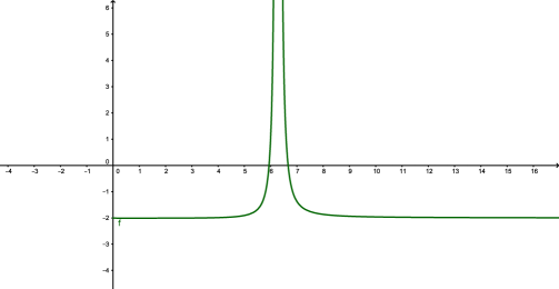
Figure 1: $c/k$ at the pole $q=1/2$ versus $\beta$ with $n=100$. The right branch corresponds to $Z>0$, i.e., the physical branch.

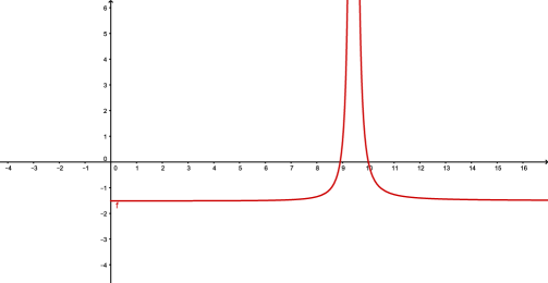
Figure 2: $c/k$ at the pole $q=2/3$ versus $\beta$, with $n=99$. The right branch corresponds to $Z>0$, i.e., the physical branch.

References

- [1] M. Gell-Mann and C. Tsallis, Eds. Nonextensive Entropy: Interdisciplinary applications, Oxford University Press, Oxford, 2004; C. Tsallis, Introduction to Nonextensive Statistical Mechanics: Approaching a Complex World, Springer, New York, 2009.
- [2] See http://tsallis.cat.cbpf.br/biblio.htm for a regularly updated bibliography on the subject.
- [3] P-Jizba, J. Korbel, V. Zatloukal, Phys. Rev. E 95, 022103 (2017); G. B. Bagci, T. Oikonomou, Phys. Rev. E 93, 022112 (2016); L. S. F. Olavo, Phys. Rev. E 64, 036125 (2001).
- [4] I. S. Oliveira: Eur. Phys. J. B 14, 43 (2000)
- [5] E. K. Lenzi , R. S. Mendes: Eur. Phys. J. B 21, 401 (2001)
- [6] C. Tsallis: Eur. Phys. J. A 40, 257 (2009)
- [7] P. H. Chavanis: Eur. Phys. J. B 53, 487 (2003)
- [8] G. Ruiz ,C. Tsallis: Eur. Phys. J. B 67, 577 (2009)
- [9] P. H. Chavanis , A. Campa: Eur. Phys. J. B 76, 581 (2010)
- [10] N. Kalogeropoulos: Eur. Phys. J. B 87, 56 (2014)
- [11] N. Kalogeropoulos: Eur. Phys. J. B 87, 138 (2014)
- [12] A. Kononovicius, J. Ruseckas: Eur. Phys. J. B 87, 169 (2014)
- [13] A. R. Plastino, A. Plastino, Phys. Lett. A 174 (1993) 384.
- [14] P. H. Chavanis, C. Sire, Physica A 356 (2005) 419; P.-H. Chavanis, J. Sommeria, Mon. Not. R. Astron. Soc. 296 (1998) 569.
- [15] D. Lynden-Bell, R. M. Lynden-Bell, Mon. Not. R. Astron. Soc. 181 (1977) 405.
- [16] C. Tsallis, Introduction to Nonextensive Statistical Mechanics (Springer, Berlin, 2009).
- [17] F. Barile et al. (ALICE Collaboration), EPJ Web Conferences 60, (2013) 13012; B. Abelev et al. (ALICE Collaboration), Phys. Rev. Lett. 111, (2013) 222301; Yu. V.Kharlov (ALICE Collaboration), Physics of Atomic Nuclei 76, (2013) 1497. ALICE Collaboration, Phys. Rev. C 91, (2015) 024609; ATLAS Collaboration, New J. Physics 13, (2011) 053033; CMS Collaboration, J. High Energy Phys. 05, (2011) 064; CMS Collaboration, Eur. Phys. J. C 74, (2014) 2847.
- [18] A. Adare et al (PHENIX Collaboration), Phys. Rev. D 83, (2011) 052004; PHENIX Collaboration, Phys. Rev. C 83, (2011) 024909; PHENIX Collaboration, Phys. Rev. C 83, (2011) 064903; PHENIX Collaboration, Phys. Rev. C 84, (2011) 044902.
- [19] A. Plastino; M. C. Rocca; G. L. Ferri: EPJB 89, 150 (2016).
- [20] A. Plastino, M. C. Rocca: arXiv:1702.03535 (2017).
- [21] C. G. Bollini and J. J. Giambiagi: Phys. Lett. B 40, (1972), 566.Il Nuovo Cim. B 12, (1972), 20.
- [22] C. G. Bollini and J.J Giambiagi : Phys. Rev. D 53, (1996), 5761.
- [23] G.’t Hooft and M. Veltman: Nucl. Phys. B 44, (1972), 189.
- [24] C. G. Bollini, T. Escobar and M. C. Rocca : Int. J. of Theor. Phys. 38, (1999), 2315.
- [25] C. G Bollini and M.C. Rocca : Int. J. of Theor. Phys. 43, (2004), 59. Int. J. of Theor. Phys. 43, (2004), 1019. Int. J. of Theor. Phys. 46, (2007), 3030.
- [26] A. Plastino, M. C. Rocca: arXiv:1701.03525
- [27] G. Livadiotis, D. J. McComas: APJ 748, 88 (2011).
- [28] G. Livadiotis: Entropy 17, 2062 (2015).
- [29] O. Obregon, International Journal of Modern Physics A 30 (2015) 1530039.
- [30] A. R. Plastino, A. Plastino, Phys. Lett. A 193 (1994) 140.
- [31] E. Verlinde, arXiv:1001.0785 [hep-th]; JHEP 04, 29 (2011).