Triad interactions and the bidirectional turbulent cascade of magnetic helicity

Abstract

Using direct numerical simulations we demonstrate that magnetic helicity exhibits a bidirectional turbulent cascade at high but finite magnetic Reynolds numbers. Despite the injection of positive magnetic helicity in the flow, we observe that magnetic helicity of opposite signs is generated between large and small scales. We explain these observations by carrying out an analysis of the magnetohydrodynamic equations reduced to triad interactions using the Fourier helical decomposition. Within this framework, the direct cascade of positive magnetic helicity arises through triad interactions that are associated with small scale dynamo action, while the occurrence of negative magnetic helicity at large scales is explained through triad interactions that are related to stretch-twist-fold dynamics and small scale dynamo action, which compete with the inverse cascade of positive magnetic helicity. Our analytical and numerical results suggest that the direct cascade of magnetic helicity is a finite magnetic Reynolds number $Rm$ effect that will vanish in the limit $Rm\to\infty$.

I Introduction

The existence of planetary and stellar magnetic fields is currently attributed to dynamo action moffatt78 ; proctorgilbert94 . One of the theoretical arguments to explain the generation and preservation of magnetic fields in spatial scales much larger than the outer scales of planets and stars is the inverse cascade of magnetic helicity in magnetohydrodynamic (MHD) turbulent flows Frischetal75 . Magnetic helicity is defined as the correlation between the magnetic field $\bm{b}\equiv\nabla\times\bm{a}$ and the magnetic potential $\bm{a}$, i.e., $H_{b}\equiv\langle{\bm{a}\cdot\bm{b}}\rangle$, with the angular brackets denoting a spatial average unless indicated otherwise. Magnetic helicity is considered to play a critical role in the long-term evolution of stellar and planetary magnetic fields brandenburg09 and hence it is important to understand its dynamics across scales in order to shed light on the saturation mechanisms of the large-scale magnetic fields of planets and stars.

Early studies using turbulent closure models Pouquet76 and mean field theory Steenbeck66 ; moffatt78 ; Krause80 have shown (within the framework of their approximations) that magnetic helicity cascades from small scales to large scales in agreement with the prediction from equilibrium statistical mechanics for the ideal MHD equations Frischetal75 . In these cases, the inverse cascade of magnetic helicity was associated with the $\alpha$ effect parker55 of large scale dynamos, where the kinetic helicity $H_{u}=\langle{\bm{u}\cdot\bm{\omega}}\rangle$ (where $\bm{u}$ denotes the velocity field and $\bm{\omega}=\nabla\times\bm{u}$ the vorticity field) generates opposite signs of magnetic helicity between large and small scales. This change in sign across scales is further supported by the magnetic helicity spectra of solar wind data Brandenburgetal11 , which show $H_{b}<0$ at small wavenumbers and $H_{b}>0$ at large wavenumbers. One way to understand this change in sign across scales is the conceptual stretch-twist-fold (STF) mechanism Childress95 ; Vainshtein72 . This mechanism proposes that the advection of magnetic field lines by a positive helical flow leads to a positive magnetic helicity at small scales and to a negative magnetic helicity at large scales since large scale magnetic field lines are twisted in the opposite direction. However, it is presently not clear if such a mechanism is directly associated with a non-linear cascade process Mininni11 .

The inverse cascade of magnetic helicity has been verified by direct numerical simulations (DNSs) meneguzzietal81 ; Brandenburg01 ; Alexakis06 at moderate values of magnetic Reynolds number $Rm$, where the small-scale magnetic helicity is dissipated quite fast. In this case, in contrast with the theory, a direct cascade of magnetic helicity with smaller magnitude was also observed. This bidirectional cascade of $H_{b}$, where an inverse and a direct cascade of magnetic helicity coexist, was observed recently even at high $Rm$ flows Mueller12 ; ld16 . In the limit of high $Rm$ concerns have been raised about the effectiveness of the $\alpha$ effect in generating large-scale magnetic fields with strong amplitude due to the detrimental feedback that fast-growing small-scale magnetic fields have on the growth rate of the large scales Vainshtein92 ; Cattaneo96 . These concerns are supported in some sense by the bidirectional cascade of magnetic helicity, because the magnitude of the inverse cascade is limited by the existence of the residual direct cascade, and by the nonlocality of the inverse cascade of magnetic helicity in the statistically stationary regime Alexakis06 ; ld16 .

In this paper, we focus on the bidirectional cascade of magnetic helicity and on the mechanism of magnetic helicity to generate opposite signs of helicity across the scales. By means of DNSs we inject mean magnetic helicity in our flows using a helical electromagnetic forcing, while the velocity field is forced by a nonhelical forcing. This is in contrast to dynamo studies, which typically force only the velocity field using a helical forcing. In dynamo studies, the kinetic helicity generates opposite signs of magnetic helicity between large and small scales. This sign change across scales makes the interpretation of statistics ambiguous. With our approach we attempt to have a dominant sign of magnetic helicity across the scales in order to avoid such ambiguities as much as possible. The interpretation of our numerical results is supported by analytical work on the triadic interactions of helical modes in MHD turbulence Linkmannetal16 ; Linkmann17b . This analysis is based on the helical decomposition of Fourier modes Craya58 ; Lesieur72 ; Herring74 , which has been an important tool to understand the cascade dynamics of helical flows in Navier-Stokes turbulence Constantin88 ; Waleffe92 ; Chen03 ; Biferale12 ; Sahoo15 ; Alexakis17 . Here, the analysis of triadic interactions of helical modes demonstrates that it can also be a useful tool to understand further (a) the presence of the direct cascade of magnetic helicity to small scales and (b) the mechanism that generates opposite signs of magnetic helicity across the scales.

This paper is organized as follows. We begin with the description of the numerical method and the resulting database in Sec. II. Sections  III and IV present the global and spectral dynamics from our numerical simulations, respectively. Our numerical results are interpreted in Sec. V in terms of the triadic interactions of helical modes, where we propose an explanation for the direct cascade of magnetic helicity and for the mechanism that generates opposite signs of magnetic helicity across the scales. We conclude in Sec. VI by summarizing our findings.

II Numerical simulations

The present work focuses on the bidirectional cascade of magnetic helicity. Thus, we consider numerical simulation of three-dimensional MHD turbulent flows forced at intermediate wavenumbers in the absence of large scales condensates. Forcing at intermediate scales and aiming for a turbulent flow with high enough scale separation poses serious computational constraints, since a very large range of scales needs to be resolved. So, to circumvent the demanding scale separation requirement and to avoid the condensation of energy at large scales, we consider high-order dissipation terms acting at the small and the large scales, respectively. These dissipation terms effectively increase the extent of the inertial range simulated for a given resolution by reducing the range of scales over which dissipation is effective. Therefore, we numerically solve the equations

$$(\partial_{t}-\nu^{-}(-1)^{m+1}\Delta^{-m}-\nu^{+}(-1)^{n+1}\Delta^{n})\bm{u} =\bm{u}\times\bm{\omega}+\bm{j}\times\bm{b}-\nabla P+\bm{f}_{u}$$

$$(\partial_{t}-\eta^{-}(-1)^{m+1}\Delta^{-m}-\eta^{+}(-1)^{n+1}\Delta^{n})\bm{b} =\nabla\times(\bm{u}\times\bm{b})\hskip 37.0pt+\bm{f}_{b}$$ (1)

where $\bm{u}$ denotes the velocity field, $\bm{b}$ the magnetic induction expressed in Alfvén units, $\bm{\omega}=\nabla\times\bm{u}$ the vorticity, $\bm{j}=\nabla\times\bm{b}$ the current density, and $P=p+|\bm{u}|^{2}/2$, with $p$ the pressure and $\bm{f}_{u}$ and $\bm{f}_{b}$ the external mechanical and electromagnetic forces, respectively. Energy is dissipated at the small scales by the terms proportional to $\nu^{+}$ and $\eta^{+}$ and at the large scales by $\nu^{-}$ and $\eta^{-}$. The indices $n$ and $m$ specify the order of the Laplacian used. In order to obtain a large inertial range, we choose $n=m=4$. In the absence of forcing and dissipation Eqs. (1) reduce to the ideal MHD equations, which conserve the total energy $E=E_{u}+E_{b}=\frac{1}{2}\langle{|\bm{u}|^{2}+|\bm{b}|^{2}}\rangle$, the magnetic helicity $H_{b}=\langle{\bm{a}\cdot\bm{b}}\rangle$ and the cross-helicity $H_{c}=\langle{\bm{u}\cdot\bm{b}}\rangle$. These conserved quantities are those that determine the turbulent cascades in our flows.

Equations (1) are solved numerically in a cubic periodic domain with sides of length $2\pi L$ using the standard pseudospectral method, which ensures that $\nabla\cdot\bm{u}=0$ and $\nabla\cdot\bm{b}=0$. Full dealiasing is achieved by the $2/3$ rule and as a result the minimum and maximum wavenumbers are $k_{box}$ = 1 and $k_{max}$ = N/3, respectively, where $N$ is the number of grid points in each Cartesian coordinate. Further details of the code can be found in Refs. Yoffe12 ; BereraLinkmann14 .

As it was mentioned above, in these simulations we choose to inject mean magnetic helicity in our flows, attempting to have a dominant sign of magnetic helicity across the scales in order to be able to interpret our results unambiguously in comparison to dynamo studies. In order to do this in a systematic way we force $\bm{b}$ using a helical forcing and $\bm{u}$ using a non-helical forcing. Here, we choose to force both $\bm{u}$ and $\bm{b}$ with the same forcing amplitude, i.e., $|\bm{f}_{u}|=|\bm{f}_{b}|$, so that both quantities are dynamically important and $\bm{b}$ has a nonlinear feedback on the flow through the Lorenz force. The forces $\bm{f}_{u}$ and $\bm{f}_{b}$ are constructed from a randomized superposition of eigenfunctions of the curl operator Brandenburg01 ; Mueller12 ; MalapakaMuller13 , resulting in Gaussian distributed and $\delta$ correlated in time forces whose helicities $\langle\bm{f}_{u,b}\cdot\nabla\times\bm{f}_{u,b}\rangle$ and correlation $\langle\bm{f}_{u}\cdot\bm{f}_{b}\rangle$ can be exactly controlled. The specific random nature of the forces ensures that at steady state the total energy input rate $\varepsilon=\varepsilon_{u}+\varepsilon_{b}=\langle\bm{u}\cdot\bm{f}_{u}\rangle+\langle\bm{b}\cdot\bm{f}_{b}\rangle\propto|\bm{f}_{u}|^{2}+|\bm{f}_{b}|^{2}$ is known a priori Novikov65 . Therefore, $\varepsilon$ can be used as a control parameter since the amplitudes of the external forces are input parameters. The external forces are chosen such that the net cross helicity in the flow is negligible by keeping the correlation $\langle{\bm{f}_{u}\cdot\bm{f}_{b}}\rangle=0$. In summary, no $H_{c}$ and no $H_{u}$ are injected into the flow, while the injection of $H_{b}$ is maximal. Here, we choose to exclude the injection of cross-helicity in the flow because we want to focus on the cascade dynamics of magnetic helicity, which can be influenced by introducing correlations between the velocity and the magnetic field Frischetal75 ; Linkmannetal16 . Finally, the initial magnetic and velocity fields are in equipartition with energy spectra peaked at the forcing wavenumber $k_{f}$ and zero helicities, i.e., $H_{b}=H_{c}=H_{u}=0$.

For all simulations, we set the magnetic Prandtl number for the small scales $Pm^{+}=\eta^{+}/\nu^{+}$ and for the large scales $Pm^{-}=\eta^{-}/\nu^{-}$ to unity, viz. $Pm^{+}=Pm^{-}=1$. The values of $\nu^{-}$ and $\eta^{-}$ are tuned such that the inverse cascade is damped before the largest scales of the system are excited while the values of $\nu^{+}$ and $\eta^{+}$ are such that $k_{max}/k_{d}\geq 1.25$ is satisfied for all the simulations, where $k_{d}\equiv(\varepsilon/(\nu^{+})^{3})^{1/(6n-2)}$ is the dissipation wavenumber BorueOrszag95 . The magnetic Reynolds number is defined based on the control parameters of the problem as $Rm_{f}\equiv Uk_{f}^{1-2n}/\eta^{+}$ with $U\equiv\left(\varepsilon/k_{f}\right)^{1/3}$.

The energy input and thus the dissipation rate $\varepsilon$ is adjusted such that $U$ is kept constant while the scale separation $k_{f}L$ increases, resulting in a set of simulations with the same Reynolds number. For simulations at $k_{f}L=10$ with different Reynolds numbers we kept the energy input constant and we varied $\nu^{+}=\eta^{+}$. All the necessary numerical parameters that make these simulations reproducible are given in Table 1 along with their total runtime $T$ of the simulations normalized by $\tau_{f}\equiv(Uk_{box})^{-1}$, a time scale defined based on the control parameters.

$k_{f}L$	$N$	$Rm_{f}$	$\nu^{+}=\eta^{+}$	$\nu^{-}=\eta^{-}$	$|\bm{f}_{u}|$	$|\bm{f}_{b}|$	$T/t_{f}$
10	128	$7\times 10^{3}$	$6.30\times 10^{-12}$	0.05	1	1	320
20	256	$7\times 10^{3}$	$4.92\times 10^{-14}$	0.05	$\sqrt{2}$	$\sqrt{2}$	130
40	512	$7\times 10^{3}$	$3.68\times 10^{-16}$	0.05	2	2	100
10	128	$7\times 10^{2}$	$6.30\times 10^{-11}$	0.05	1	1	90
10	256	$9\times 10^{4}$	$4.92\times 10^{-14}$	0.05	1	1	110

Table 1: Numerical parameters of the simulations. Note that $k_{f}$ denotes the forcing wave number, $T$ is the total runtime in simulation units, $|\bm{f}_{u}|$ and $|\bm{f}_{b}|$ are the mechanical and electromagnetic forcing magnitudes, respectively, and $t_{f}\equiv(Uk_{box})^{-1}$ a time scale defined based on the control parameters. All simulations are well resolved with $k_{cut}/k_{d}\geqslant 1.25$. The hyperdissipative Reynolds number is defined as $Rm_{f}=Uk_{f}^{1-2n}/\eta^{+}$.

III Time evolution

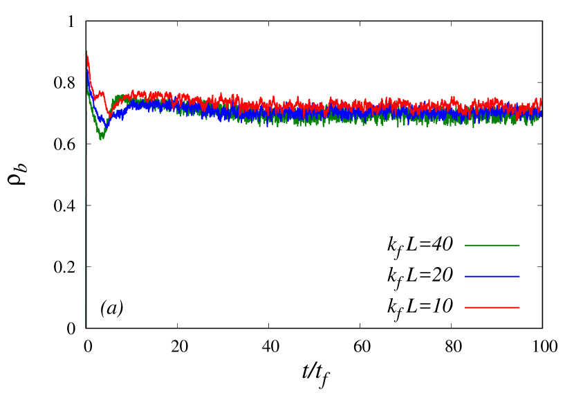
Before discussing the interaction of the helical modes in order to understand further the dynamics of magnetic helicity across scales, we provide an overview of the statistics of the flows under study. In Fig. 1(a) we have plotted the time evolution of the normalized magnetic helicity

$$\rho_{b}\equiv H_{b}/(\langle{|\bm{a}|^{2}}\rangle\langle{|\bm{b}|^{2}}\rangle)^{1/2},$$ (2)

which belongs to the range $-1\leq\rho_{b}\leq 1$. For $\rho_{b}=0$ the flows have no magnetic helicity, while for $\rho_{b}=\pm 1$ the flows are fully dominated by magnetic helicity, which means that the Lorentz force $\bm{j}\times\bm{b}$ is expected to be zero on average. At time $t=0$, we set $\rho_{b}=0$ but instantaneously it reaches high values because of the direct injection of positive $H_{b}$ by the helical electromagnetic force. At steady state $\rho_{b}$ reaches a mean value of 0.7 for all the flows with scale separations $k_{f}L=10,20,40$, indicating that the flows are dominated to a large degree by positive mean magnetic helicity.

The strength of the direct and the inverse cascade of magnetic helicity at steady state can be quantified by the rate of dissipation in large scales $\varepsilon_{H_{b}}^{-}$ and small scales $\varepsilon_{H_{b}}^{+}$ as

$$\varepsilon_{H_{b}}^{\pm}\equiv\nu^{\pm}\langle{\bm{a}\cdot\Delta^{\pm n}\bm{b}}\rangle.$$ (3)

Then, the total magnetic helicity dissipation can be computed as the sum of the dissipation at large and small scales, viz., $\varepsilon_{H_{b}}=\varepsilon_{H_{b}}^{-}+\varepsilon_{H_{b}}^{+}$. In Fig. 1(b), we plot the time-series of the ratio $\varepsilon_{H_{b}}^{-}/\varepsilon_{H_{b}}$ for the three scale separations that we simulated (see Table 1). The values of $\varepsilon_{H_{b}}^{-}/\varepsilon_{H_{b}}$ can range from 0 to 1. For $\varepsilon_{H_{b}}^{-}/\varepsilon_{H_{b}}=0$ there is no inverse cascade of magnetic helicity, while for $\varepsilon_{H_{b}}^{-}/\varepsilon_{H_{b}}=1$ there is no direct cascade of magnetic helicity.

(a)

(b)

Figure 1: Time series of (a) the normalized magnetic helicity $\rho_{b}$ and (b) the ratio $\varepsilon_{H_{b}}^{-}/\varepsilon_{H_{b}}$ for flows with scale separations $k_{f}L=10,20$ and 40.

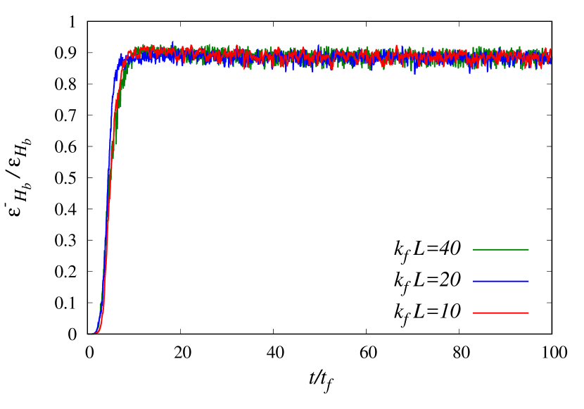
In the initial transient regime the amount of magnetic helicity that is transferred to the large scales increases monotonically until large scale dissipation takes place and the ratio $\varepsilon_{H_{b}}^{-}/\varepsilon_{H_{b}}$ saturates to the value of 0.9 (see Fig. 1(b)). This clearly shows that there is a bidirectional cascade of $H_{b}$ with 90% of the magnetic helicity cascading to the large scales at steady state while 10% of the magnetic helicity cascades towards the small scales since $\varepsilon_{H_{b}}^{+}/\varepsilon_{H_{b}}\simeq 0.1$. The bidirectional cascade of Hb had been observed qualitatively in Refs. Alexakis06 ; Mueller12 and it was quantified in Ref. ld16 . As scale separation increases the amount of magnetic helicity that cascades to the large and small scales remains fixed in contrast to the cascade of the total energy, where $\varepsilon^{-}/\varepsilon\propto(k_{f}L)^{-1}$ as it was shown in ld16 , with the total energy dissipation rate being $\varepsilon=\varepsilon^{-}+\varepsilon^{+}$ and $\varepsilon^{\pm}\equiv\eta^{\pm}\langle{|\nabla^{\pm n}\bm{b}|^{2}}\rangle+\nu^{\pm}\langle{|\nabla^{\pm n}\bm{u}|^{2}}\rangle$. Thus, for $k_{f}L\gg 1$ we expect the ratio $\varepsilon^{-}/\varepsilon\rightarrow 0$, implying that the total energy will cascade only toward the small scales while the direct cascade of magnetic helicity will not vanish because $\varepsilon_{H_{b}}^{+}/\varepsilon_{H_{b}}$ is expected to remain finite as our numerical simulations suggest.

However, for fixed $k_{f}L$ it is plausible that the direct cascade of magnetic helicity vanishes in the high-magnetic-Reynolds-number limit. This can be inferred by considering the following upper bound derived in Ref. da15 for the magnitude of the total dissipation rate of magnetic helicity at small scales for the MHD equations that involve dissipation terms with Laplacian operators (i.e., the exponent $n=1$)

$$|\varepsilon_{H_{b}}|\equiv\eta|\langle\bm{a}\cdot\Delta\bm{b}\rangle|=\eta|\langle{\bm{b}\cdot\bm{j}}\rangle|\leq\eta\langle{|\bm{b}|^{2}}\rangle^{1/2}\langle{|\bm{j}|^{2}}\rangle^{1/2}\leq\eta^{1/2}\langle{|\bm{b}|^{2}}\rangle^{1/2}\varepsilon^{1/2}\ ,$$ (4)

where $\varepsilon=\eta\langle{|\bm{j}|^{2}}\rangle+\nu\langle{|\bm{\omega}|^{2}}\rangle$ is the total energy dissipation rate in this case, $\eta$ is the magnetic resistivity, and $\nu$ is the kinematic viscosity. In high-Reynolds-number MHD turbulence, $\varepsilon$ becomes finite and independent of $\eta$ and $\nu$ Mininni09 ; Dallas14b ; Linkmann17a . Thus, in the limit of $\eta\to 0$ Eq. (4) suggests that $|\varepsilon_{H_{b}}|\to 0$, unless $\langle{|\bm{b}|^{2}}\rangle\propto 1/\eta$, implying infinite magnetic energy.

A similar inequality for the dissipation rate of magnetic helicity at small scales for Eqs. (1), which involve higher-order dissipation terms, can be derived as

$$|\varepsilon_{H_{b}}^{+}|\equiv\eta^{+}|\langle\bm{a}\cdot\Delta^{n}\bm{b}\rangle|=\eta^{+}|\langle\bm{b}\cdot\Delta^{n-1}\bm{j}\rangle|\leqslant\eta^{+}\langle{|\bm{b}|^{2}}\rangle^{1/2}\langle|\Delta^{n-1}\bm{j}|^{2}\rangle^{1/2}.$$ (5)

Note that for $n=1$ we recover Eq. (4), however, for $n>1$ the term $\langle{|\Delta^{n-1}\bm{j}|^{2}}\rangle$ cannot be directly related to the small-scale dissipation rate of magnetic energy $\varepsilon_{b}^{+}\equiv\eta^{+}\langle{\bm{b}\cdot\Delta^{n}\bm{b}}\rangle=\eta^{+}\langle{|\nabla^{n-1}\bm{j}|^{2}}\rangle$. Therefore, to make any conclusions, if any, for the behavior of $|\varepsilon_{H_{b}}^{+}|$ in the limit of $\eta^{+}\rightarrow 0$, we need to compute the scaling of $\varepsilon_{H_{b}}^{+}$ with $\eta^{+}$ as we cannot make any a priori statements like in Eq. (4). For this purpose, we performed three simulations with the same scale separation $k_{f}L=10$ but different $Rm_{f}$. These preliminary results are plotted in Fig. 2, which shows that $\varepsilon_{H_{b}}^{+}$ normalized by the total dissipation of magnetic helicity $\varepsilon_{H_{b}}$ has a weak power-law behavior in terms of $Rm_{f}$, i.e. $\varepsilon_{H_{b}}^{+}/\varepsilon_{H_{b}}\propto Rm_{f}^{-0.22}$. This scaling suggests that the direct cascade of magnetic helicity may not persist in the limit of $Rm_{f}\to\infty$. However, further investigation into this issue is necessary in order to understand this scaling law and the small-scale dynamics of the magnetic helicity.

Figure 2: Dependence of $\varepsilon_{H_{b}}^{+}/\varepsilon_{H_{b}}$ on the magnetic Reynolds number $Rm_{f}$ for the flows with scale separation $k_{f}L=10$.

IV Spectral dynamics

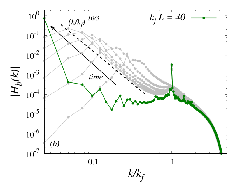
After considering the global dynamics and the time evolution of our flows, we now elaborate on the spectral dynamics of magnetic helicity in order to have a clear picture of the dynamics across scales. This is best demonstrated by looking at the spectrum of magnetic helicity $H_{b}(k)$ and its normalized flux $\Pi_{H_{b}}(k)/\varepsilon_{H_{b}}$ for the flow with scale separation $k_{f}L=40$ (see Fig. 3). The magnetic helicity flux is defined as

$$\Pi_{H_{b}}(k)=\sum_{k^{\prime}=1}^{k}\sum_{|\bm{k}|=k^{\prime}}\hat{\bm{b}}_{\bm{k}}^{*}\cdot\widehat{(\bm{u}\times\bm{b})}_{\bm{k}}\ ,$$ (6)

and the magnetic helicity spectrum as $H_{b}(k)=\sum_{|\bm{k}|=k}\hat{\bm{a}}_{\bm{k}}^{*}\cdot\hat{\bm{b}}_{\bm{k}}$, where the caret denotes the Fourier modes of the corresponding real vector fields and the asterisk the complex conjugate.

(a)

(b)

Figure 3: (a) Magnetic helicity flux $\Pi_{H_{b}}(k)$ normalized by $\varepsilon_{H_{b}}$ and (b) absolute value of the magnetic helicity spectrum $|H_{b}(k)|$ for a flow with scale separation $k_{f}L=40$. The light gray curves denote instantaneous quantities at the transient regime of the flow for $0.5\leqslant t/t_{f}\leqslant 3$, while the green (dark gray) curve denotes the time-averaged profile in the steady-state regime.

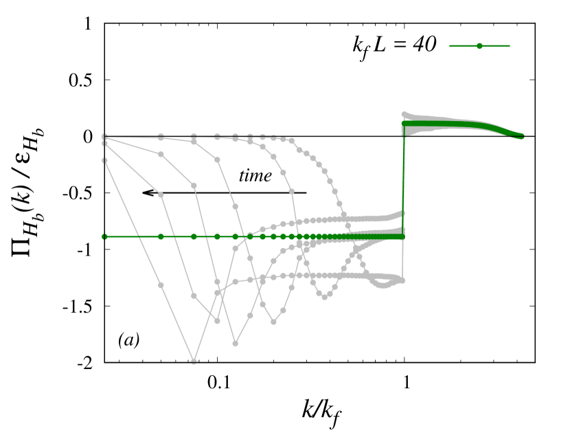
The gray curves denote instantaneous profiles at the transient regime of the flow while the green (dark gray) curves denote the time-averaged profiles at the steady state regime. Negative values of the magnetic helicity flux imply upscale transfer while positive values imply downscale transfer. Thus, Fig. 3(a) shows clearly the bidirectional cascade behavior of magnetic helicity with most of $H_{b}$ cascading towards large scales in agreement with Fig. 1(b). The gray curves indicate how the flux builds up at the transient state and of course these curves do not satisfy the balance $\Pi_{H_{b}}(k)=\varepsilon_{H_{b}}$, which is only expected to be valid on average over a statistically stationary regime.

At the transient stage of the simulation the inverse and the direct cascade of magnetic helicity is dominated by local interactions, as it has already been reported Alexakis06 . Before the flow saturates to a steady-state solution a spectrum with a negative power-law slope can be observed at low wave numbers. The scaling of this spectrum was proposed to be $H_{b}(k)\propto k^{-10/3}$ Mueller12 ; Mininni09 , which agrees with our data. However, if one integrates further in time the spectrum develops even more as the flow saturates to a statistically stationary regime. In this regime, most of the magnetic helicity is concentrated at the largest scales [see also the spectrum of normalized helicity $\rho_{b}(k)$ in Fig. 5(a)] and the inverse cascade of $H_{b}$ becomes nonlocal in wave-number space, i.e., $H_{b}$ is transferred directly from the forced scale to the largest scales of the flow, while the forward cascade remains local ld16 ; Alexakis06 ; Brandenburg01 . This transition to nonlocal interactions at steady state occurs when condensation takes place at the largest scale of the system. In this case, the large-scale vortex interacts directly with the small-scale vortices of the flow (i.e., nonlocally in wave-number space) ld16 . This behavior is also observed in confined two-dimensional hydrodynamic turbulent flows shuklaetal16 ; xiaetal08 . Finally, the scaling of the time-averaged spectrum of magnetic helicity at steady state is $H_{b}(k)\propto k^{0}$ for wave numbers $k<k_{f}$, suggesting that the large scales behave as if they were in absolute equilibrium ld16 . Now, the scaling for $k>k_{f}$ seems to be $H_{b}(k)\propto k^{-5/3}$. However, this is not conclusive from the plot due to the limited spectral range and the high-order dissipative terms that act at the largest wave numbers.

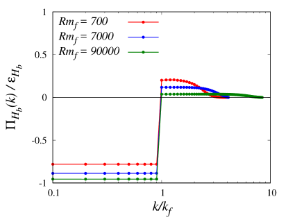
The behavior of the magnetic helicity flux $\Pi_{H_{b}}(k)$ at steady-state with increasing $Rm_{f}$ is presented in Fig. 4. As can be seen from the figure, the small-scale range where $\Pi_{H_{b}}(k)\simeq\varepsilon_{H_{b}}^{+}$ extends over a larger range of wave numbers successively with increasing $Rm_{f}$ as expected for a cascade process. However, the height of the plateau, i.e., the value of $\varepsilon_{H_{b}}^{+}$, decreases with increasing $Rm_{f}$, as quantified in Fig. 2.

Figure 4: Spectral flux of magnetic helicity normalised by its dissipation rate $\Pi_{H_{b}}(k)/\varepsilon_{H_{b}}$ at different values of $Rm_{f}$ for the flows with scale separation $k_{f}L=10$. The amplitude of the cascade at $k/k_{f}>1$ is quantified as a function of $Rm_{f}$ in Fig. 2.

The purpose of our simulations using a positively helical electromagnetic force was to impose a mean magnetic helicity in our flows with the intention to have a dominant sign of magnetic helicity across the scales. However, at the steady-state regime of our simulations there are low-wave-number modes that develop a negative sign of magnetic helicity even though the mean value of magnetic helicity is positive in the flow. This is clearly depicted in Fig. 5(a), where we plot the time-averaged spectra of the normalized magnetic helicity $\rho_{b}(k)$ for flows with $k_{f}L=10,20,40$.

(a)

(b)

Figure 5: (a) Time-averaged relative magnetic helicity spectra $\rho_{b}(k)$ and (b) time-averaged relative kinetic helicity spectra $\rho_{u}(k)$ for flows with scale separations $k_{f}L=10,20$, and 40.

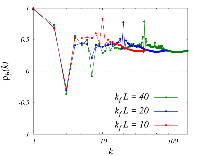
Note that all the flows generate negative $\rho_{b}(k)$ at wave number $k=3$, which indicates that there is a consistent mechanism generating opposite signs of helicity across the scales even in these flows that are dominated by positive net magnetic helicity. Moreover, we observe that the number of modes at $k<k_{f}$ with negative magnetic helicity increases as the scale separation $k_{f}L$ increases.

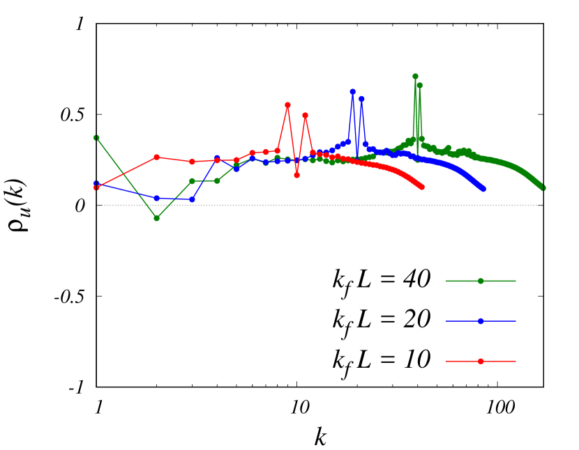
Despite the nonhelical mechanical forcing, a whole spectrum of positive kinetic helicity is observed across the scales. This is shown in Fig. 5(b), where we plot the spectra of the relative kinetic helicity $\rho_{u}(k)\equiv H_{u}(k)/(\langle{|{\hat{\bm{u}}}_{\bm{k}}|^{2}}\rangle\langle{|{\hat{\bm{\omega}}}_{\bm{k}}|^{2}}\rangle)^{1/2}$ for the flows with $k_{f}L=10,20,$ and $40$. The values of $\rho_{u}(k)$ for wave numbers $k<k_{f}$ decrease as the scale separation $k_{f}L$ increases, while they are particularly high close to the forcing scale where $\rho_{b}(k)$ is also dominant. This correlation seems to be related to the injection of positive magnetic helicity in the flow. In order to understand further the observations from our numerical simulation on the generation of the $\rho_{u}(k)$ spectrum, the direct cascade of magnetic helicity, and the mechanism that generates opposite signs of magnetic helicity between large and small scales, we study analytically the triadic interactions of helical modes in the following section.

V Triad interactions of helical modes

The three-dimensional vector fields of the velocity and the magnetic field are solenoidal (viz., $i\bm{k}\cdot{\hat{\bm{u}}}_{\bm{k}}=0$ and $i\bm{k}\cdot{\hat{\bm{b}}}_{\bm{k}}=0$), hence ${\hat{\bm{u}}}_{\bm{k}}$ and ${\hat{\bm{b}}}_{\bm{k}}$ must lie in the plane perpendicular to the wave vector $\bm{k}$. This plane is spanned by two eigenvectors of the curl operator in Fourier space with nonzero eigenvalues. Since these eigenvectors are by definition fully helical, each Fourier mode ${\hat{\bm{u}}}_{\bm{k}}$ and ${\hat{\bm{b}}}_{\bm{k}}$ can be further decomposed into two modes with positive and negative helicity

$${\hat{\bm{u}}}_{\bm{k}}(t) =u^{+}_{\bm{k}}(t){\bm{h}}^{+}_{\bm{k}}+u^{-}_{\bm{k}}(t){\bm{h}}^{-}_{\bm{k}}=\sum_{s_{k}}u^{s_{k}}_{\bm{k}}(t){\bm{h}}^{s_{k}}_{\bm{k}}\ ,$$ (7)

$${\hat{\bm{b}}}_{\bm{k}}(t) =b^{+}_{\bm{k}}(t){\bm{h}}^{+}_{\bm{k}}+b^{-}_{\bm{k}}(t){\bm{h}}^{-}_{\bm{k}}=\sum_{\sigma_{k}}b^{\sigma_{k}}_{\bm{k}}(t){\bm{h}}^{\sigma_{k}}_{\bm{k}}\ ,$$ (8)

where the basis vectors $\bm{h}^{\pm}_{\bm{k}}$ are the orthonormal eigenvectors of the curl operator in Fourier space satisfying $i\bm{k}\times{\bm{h}}^{s_{k}}_{\bm{k}}=s_{k}|\bm{k}|{\bm{h}}^{s_{k}}_{\bm{k}}$ with $s_{k}=\pm$ and $\sigma_{k}=\pm$. This is the so-called helical decomposition Craya58 ; Lesieur72 ; Herring74 . To study the triad interaction of helical modes, we use the formalism that was developed by Waleffe Waleffe92 for the Navier-Stokes equations and extended by Linkmann et al. Linkmannetal16 ; Linkmann17b to the MHD equations. This is essentially a linear stability analysis of a dynamical system obtained from the MHD equations in the limits of $\nu\to 0$ and $\eta\to 0$. In the MHD equations that are shown here in Fourier space

$$(\partial_{t}+\nu k^{2})\hat{\bm{u}}_{\bm{k}}= -\mathcal{F}\left[\nabla\left(p+\frac{|\bm{u}|^{2}}{2}\right)\right]+\sum_{\bm{k}+\bm{p}+\bm{q}=0}\left((-i{\bm{p}}\times\hat{\bm{u}}_{\bm{p}})^{*}\times\hat{\bm{u}}_{\bm{q}}^{*}+(i\bm{p}\times\hat{\bm{b}}_{\bm{p}})^{*}\times\hat{\bm{b}}_{\bm{q}}^{*}\right)\ ,$$ (9)

$$(\partial_{t}+\eta k^{2})\hat{\bm{b}}_{\bm{k}}= \ i\bm{k}\times\sum_{\bm{k}+\bm{p}+\bm{q}=0}\hat{\bm{u}}_{\bm{p}}^{*}\times\hat{\bm{b}}_{\bm{q}}^{*}\ ,$$ (10)

with $\mathcal{F}$ denoting the Fourier transform as a linear operator, the convolutions that describe the respective Fourier transforms of the inertial term $\bm{u}\times\bm{\omega}$, the Lorentz force $\bm{j}\times\bm{b}$, and the curl of the electromotive force $\nabla\times(\bm{u}\times\bm{b})$ are reduced to single triads of wave vectors $\bm{k}$, $\bm{p},$ and $\bm{q}$ satisfying $\bm{k}+\bm{p}+\bm{q}=0$. For convenience and without loss of generality we impose the ordering $|\bm{k}|\leq|\bm{p}|\leq|\bm{q}|$. In order to study the dynamics in the inertial range of scales, the dissipation terms are neglected in the limits of $\nu\to 0$ and $\eta\to 0$. Following Lessinnes et al. Lessinnes09 , by substituting Eqs. (7) and (8) into Eqs. (9) and (10) after restricting the convolutions to single triads and subsequently taking the inner product with the helical basis vectors, one can then derive the following system of ordinary differential equations, which conserves the ideal invariants of the MHD equations Lessinnes09 :

$$\partial_{t}{u^{s_{k}}_{\bm{k}}}^{*} =g_{s_{k}s_{p}s_{q}}(s_{p}p-s_{q}q)\>u^{s_{p}}_{\bm{p}}u^{s_{q}}_{\bm{q}}-g_{s_{k}\sigma_{p}\sigma_{q}}(\sigma_{p}p-\sigma_{q}q)\>b^{\sigma_{p}}_{\bm{p}}b^{\sigma_{q}}_{\bm{q}}\ ,$$

$$\partial_{t}{u^{s_{p}}_{\bm{p}}}^{*} =g_{s_{k}s_{p}s_{q}}(s_{q}q-s_{k}k)\>u^{s_{q}}_{\bm{q}}u^{s_{k}}_{\bm{k}}-g_{\sigma_{k}s_{p}\sigma_{q}}(\sigma_{q}q-\sigma_{k}k)\>b^{\sigma_{q}}_{\bm{q}}b^{\sigma_{k}}_{\bm{k}}\ ,$$

$$\partial_{t}{u^{s_{q}}_{\bm{q}}}^{*} =g_{s_{k}s_{p}s_{q}}(s_{k}k-s_{p}p)\>u^{s_{k}}_{\bm{k}}u^{s_{p}}_{\bm{p}}-g_{\sigma_{k}\sigma_{p}s_{q}}(\sigma_{k}k-\sigma_{p}p)\>b^{\sigma_{k}}_{\bm{k}}b^{\sigma_{p}}_{\bm{p}}\ ,$$

$$\partial_{t}{b^{\sigma_{k}}_{\bm{k}}}^{*} =\sigma_{k}k\>\left(g_{\sigma_{k}\sigma_{p}s_{q}}b^{\sigma_{p}}_{\bm{p}}u^{s_{q}}_{\bm{q}}-g_{\sigma_{k}s_{p}\sigma_{q}}u^{s_{p}}_{\bm{p}}b^{\sigma_{q}}_{\bm{q}}\right)\ ,$$

$$\partial_{t}{b^{\sigma_{p}}_{\bm{p}}}^{*} =\sigma_{p}p\>\left(g_{s_{k}\sigma_{p}\sigma_{q}}b^{\sigma_{q}}_{\bm{q}}u^{s_{k}}_{\bm{k}}-g_{\sigma_{k}\sigma_{p}s_{q}}u^{s_{q}}_{\bm{q}}b^{\sigma_{k}}_{\bm{k}}\right)\ ,$$

$$\partial_{t}{b^{\sigma_{q}}_{\bm{q}}}^{*} =\sigma_{q}q\>\left(g_{\sigma_{k}s_{p}\sigma_{q}}b^{\sigma_{k}}_{\bm{k}}u^{s_{p}}_{\bm{p}}-g_{s_{k}\sigma_{p}\sigma_{q}}u^{s_{k}}_{\bm{k}}b^{\sigma_{p}}_{\bm{p}}\right)\ ,$$ (11)

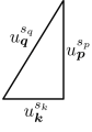
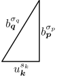
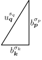
where the geometric factors $g$ describe the coupling between the helical basis vectors, i.e. $g_{s_{k}s_{p}s_{q}}={\bm{h}}^{s_{k}}_{\bm{k}}\cdot({{\bm{h}}^{s_{p}}_{\bm{p}}}\times{{\bm{h}}^{s_{q}}_{\bm{q}}})$ Waleffe92 . Further details on the full derivation of Eqs. (V) can be found in Refs. Lessinnes09 ; Linkmannetal16 ; Linkmann17b . A graphical representation of the system of equations (V) is shown in Fig. 6, where each convolution term corresponds to a triangle that represents a triad of wave vectors. Note that two triads are required to describe the interactions that correspond to the term $\nabla\times(\bm{u}\times\bm{b})$ due to a necessary symmetrization of the convolution in Fourier space. However, this symmetrization does not allow one to disentangle the triadic interactions of the advection term $\bm{u}\cdot\nabla\bm{b}$ and the stretching term $\bm{b}\cdot\nabla\bm{u}$ of the magnetic field Linkmannetal16 . Different interactions of helical modes can now be studied via Eqs. (V) by choosing different combinations of $s_{k},s_{p},s_{q}$ and $\sigma_{k},\sigma_{p},\sigma_{q}$.

Figure 6: Graphical representation of the dynamical system given by Eqs. (V) consisting of the coupling among velocity (left) and magnetic-velocity (right) triadic interactions as in Ref. Linkmann17b . The magnetic-velocity interactions correspond to several terms in Eqs. (V), depending on whether the time evolution of the velocity or the magnetic field modes is considered.

A linear stability analysis of steady solutions of Eqs. (V) has been carried out by Linkmann et al. Linkmannetal16 , where a linear instability corresponds to a transfer of energy from the unstable helical mode (denoted in capital letters) of a single triad interaction to the perturbations (denoted in lower case letters), i.e., to the other two helical modes of the triad. Under the assumption that the statistical behavior of the flow is controlled by the stability characteristics of these isolated triads (referred to as the instability assumption) Kraichnan67 ; Waleffe92 , it is possible to draw conclusions concerning the energy and helicity transfer in the MHD equations from the stability properties of Eqs. (V). Different physical processes such as the inverse cascade of magnetic helicity or kinematic dynamo action can then be studied on the level of triad interactions by setting up specific perturbation problems Linkmannetal16 . Depending on the characteristic wave numbers and the sign of helicities of the interacting modes, the dominant interscale energy transfers can then be identified through a comparison of the growth rates of the perturbations Linkmann17b .

If we consider a steady solution for the velocity field subject to magnetic perturbations, it is possible to identify all the triadic interactions of helical modes that produce small as well as large scale growth of the magnetic field (see Ref. Linkmannetal16 for details). With this result Linkmann et al. Linkmann17b were able to interpret how small- and large-scale dynamos operate at the level of triadic interactions. In Fig. 7 we present all the triads that lead to linear instabilities and hence to energy transfer,

(a)

(b)

(c)

(d)

(e)

(f)

Figure 7: Triadic interactions of helical modes leading to energy transfers when considering a steady solution for the velocity field subject to magnetic perturbations. Blue (dark gray) arrows indicate small-scale dynamos and red (light gray) arrows indicate large-scale dynamos. The thickness of the arrows indicates the magnitude of the transfer.

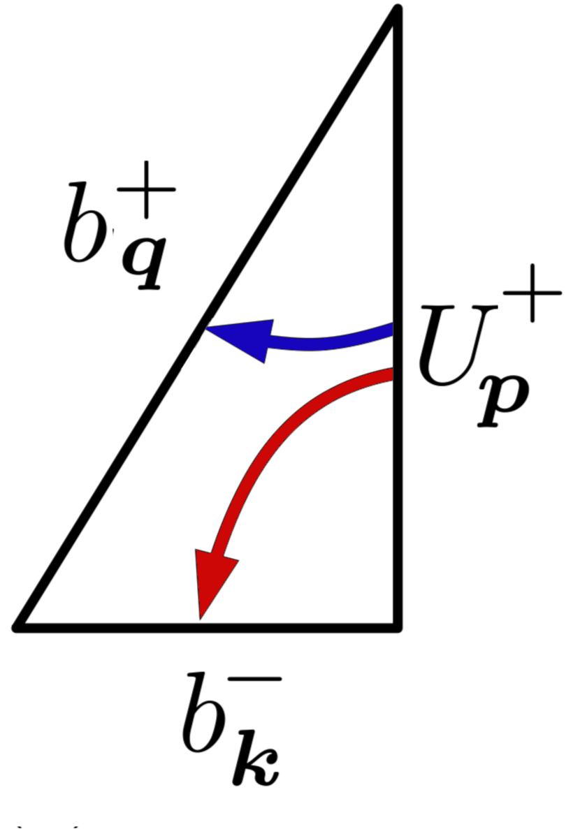
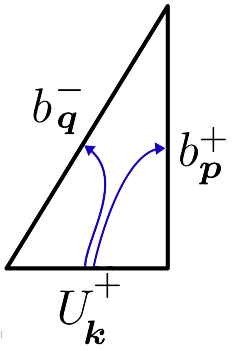
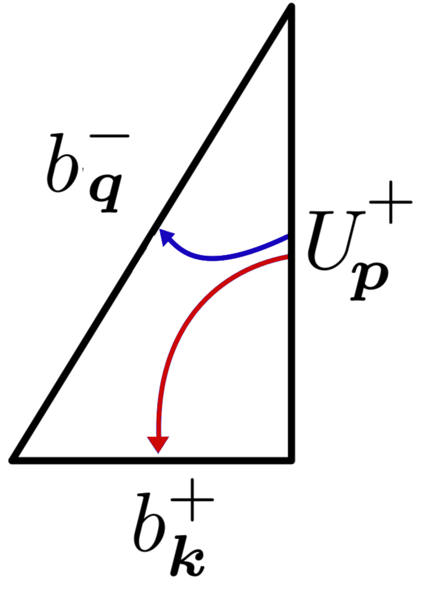
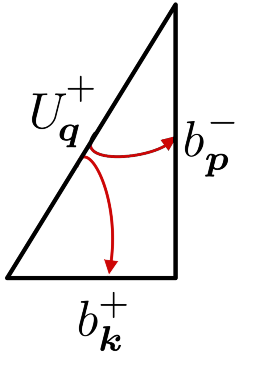
where the red arrows indicate large-scale dynamo action (i.e., energy is transferred to small-wavenumber helical modes of the magnetic field), the blue arrows indicate small-scale dynamo action (i.e., energy is transferred to large-wavenumber helical modes of the magnetic field), and the thickness of the arrows indicates the magnitude of the transfer (see Refs. Linkmannetal16 ; Linkmann17b for details). More precisely, the thickness of the arrows is qualitative, reflecting that for any nontrivial triad geometry the growth rates of the perturbations have a consistent ordering [see, e.g., Eq. (20)].

Similarly, if we consider the linear stability analysis of a steady solution for the magnetic field subject to velocity and magnetic perturbations, one can obtain the triadic interactions involving unstable helical modes shown in Fig. 8,

(a)

(b)

(c)

(d)

(e)

(f)

Figure 8: Triadic interactions of helical modes leading to energy transfer when considering a stable solution for the magnetic field subject to velocity and magnetic perturbations. Green (light gray) arrows indicate an inverse transfer of magnetic helicity and magenta (dark gray) arrows indicate conversion of magnetic to kinetic energy due to the Lorentz force. The thickness of the arrows indicates the magnitude of the transfer.

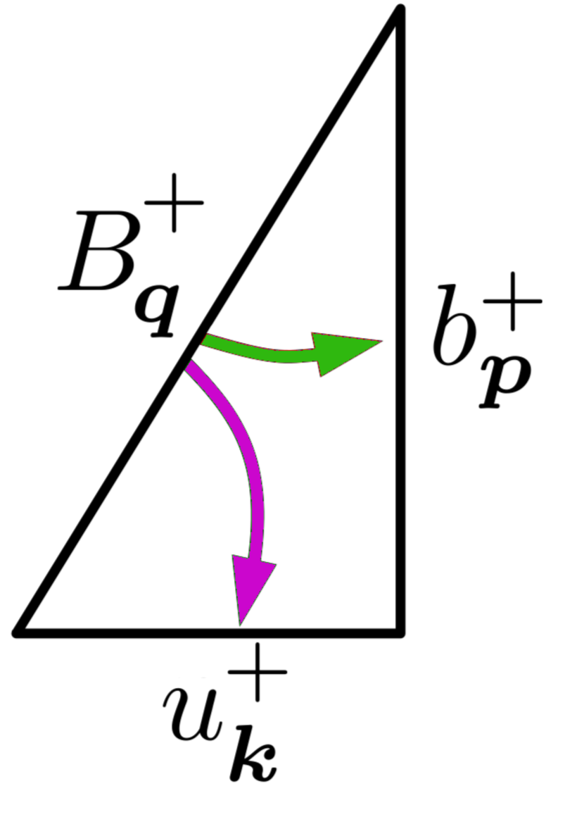
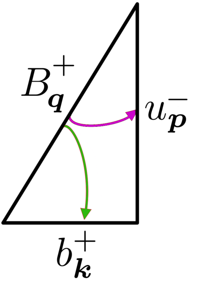
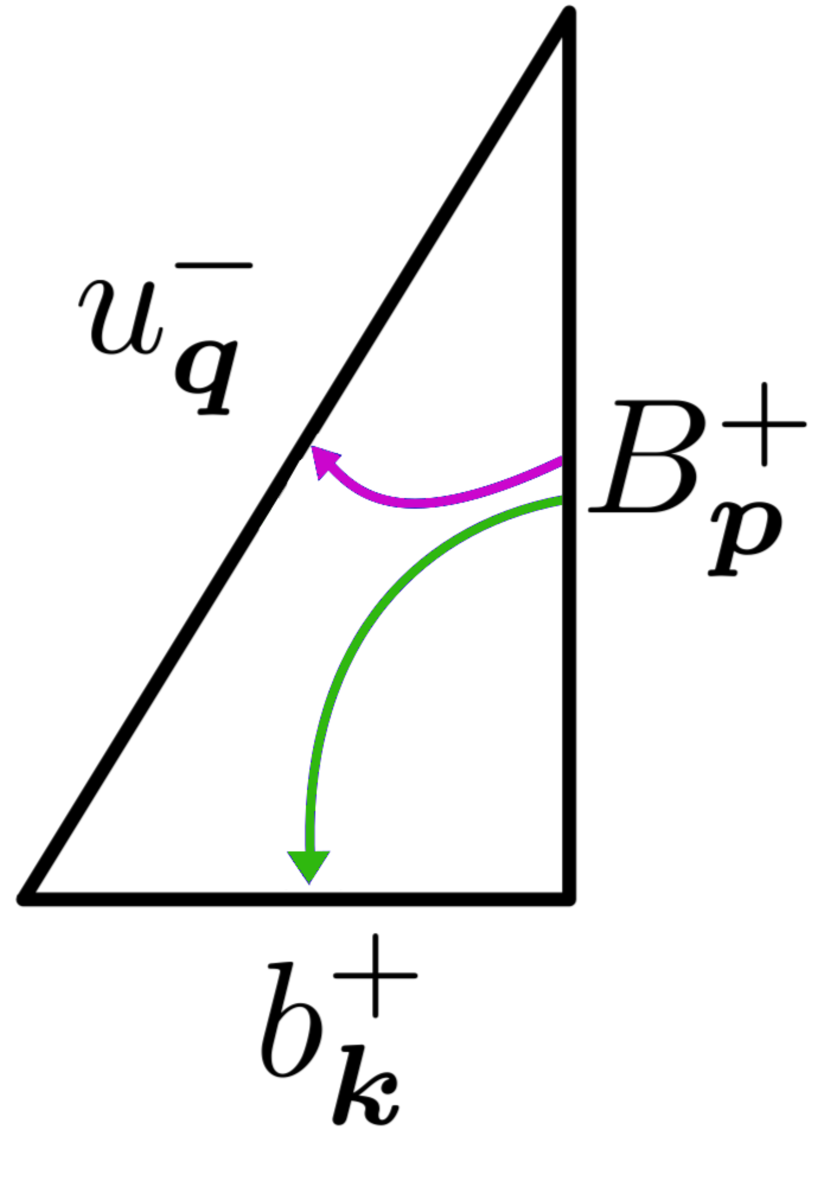
where the green arrows indicate magnetic energy transfer, the magenta arrows indicate the conversion of magnetic to kinetic energy due to the action of the Lorentz force, and the thickness of the arrows indicates the magnitude of the transfer. As can be seen in Fig. 8, triadic interactions of helical modes leading to energy transfer occur only if (a) the steady solution of the magnetic field and the magnetic perturbation have the same sign of magnetic helicity, and (b) the characteristic wave number of the magnetic perturbation is smaller than the characteristic wavenumber of the steady solution. In other words, the energy transfer between the magnetic modes occurs exclusively from large to small wavenumbers and only between magnetic modes with the same sign of helicity, which implies an inverse cascade of magnetic helicity Linkmannetal16 . As indicated by the thickness of the green arrows, the inverse cascade of magnetic helicity is stronger if the magnetic and kinetic helicities are of the same sign Linkmann17b . Following the analysis that was carried out in Ref. Linkmann17b for the triadic interactions corresponding to kinematic dynamo action and the inverse transfer of magnetic helicity, we carry out an analysis of the relative magnitude of the growth rates corresponding to triad interactions of the Lorentz force in the Appendix. Our analysis shows that the conversion of magnetic to kinetic energy through the Lorentz force occurs mainly between helical modes of the velocity and the magnetic field that have the same sign of helicity, as indicated by the thick magenta arrows in Fig. 8.

V.1 Direct cascade of magnetic helicity

In order to understand the presence of the direct cascade of positive magnetic helicity, observed in our simulations, at the level of triadic interactions, we aim to identify interactions among helical modes that transfer energy to helical modes of positive magnetic helicity at large wavenumbers. The only possible way to get such interactions is via the triads in Figs. 7(a), 7(b), and 7(d). From these three triad interactions, those that dominate the small scales are shown in Figs. 7(a) and 7(b), where the unstable helical modes $U_{\bm{k}}^{+}$ and $U_{\bm{p}}^{+}$ transfer energy to $B_{\bm{q}}^{+}$ via transfers that represent a small scale dynamo. In all these cases, energy is transferred from a small-wave-number mode to a large-wave-number mode and this transfer originates from a positively helical unstable mode of the velocity field. As we have already observed from our simulations, kinetic helicity has a well-defined spectrum [see Fig. 5(b)] and thus positively helical modes of the velocity field are present and can enable such triadic interactions.

The generation of kinetic helicity in these flows can be understood via the triadic interactions of Fig. 8(a)-8(c). These three triads are the dominant interactions in this linear stability analysis and in all these cases modes of positive magnetic helicity generate modes of positive kinetic helicity. In other words, the analysis of triadic interactions suggests that the magnetic helicity generates kinetic helicity through triad interactions associated with the Lorentz force. As discussed in Sec. III, our flows are dominated by positively helical modes of the magnetic field because we maintain positive net magnetic helicity [see Fig. 1(a)] via the positively helical electromagnetic force $\bm{f}_{b}$.

In summary, since there is no direct transfer of energy between modes that have opposite sign of magnetic helicity, the only way for a direct cascade of $H_{b}$ to occur is via the Lorentz force, which generates modes with positive kinetic helicity. These in turn excite modes with both positive and negative magnetic helicity with the dominant interactions creating positively helical magnetic-field modes at small scales (see Figs. 7(a), 7(b), and 7(d)).

V.2 Negative magnetic helicity at large scales

Here we discuss the triad interactions that lead to the generation of modes with negative magnetic helicity at small wave numbers. As stated above, there is no direct transfer of energy between modes that have opposite sign of magnetic helicity. Therefore, the triad interactions that generate opposite signs of magnetic helicity between large and small scales have to involve a transfer of energy from positively helical modes of the velocity field. According to the results of the stability analysis of the triadic interactions shown in Figs. 7 and 8, we can conclude that there are two types of instabilities leading to the occurrence of large-scale magnetic helicity, namely, triadic instabilities that represent large-scale dynamo, including STF dynamics [see Figs. 7(b) and 7(c)], and those that can be directly associated with the inverse cascade of positive magnetic helicity [see Figs. 8(b) and 8(c)]. Here we expect a competition between triad interactions in Figs. 7(b) and 7(c) and those in Figs. 8(b) and 8(c). Based on our numerical simulations, we observe the persistent generation of negative magnetic helicity at wave number $k=3$ [see Fig. 5(a)] despite the positive mean value of magnetic helicity that is maintained by the positively helical electromagnetic forcing. This observation indicates that the triad interactions of Figs. 7(b) and 7(c) dominate over Figs. 8(b) and 8(c) at low wavenumbers as the scale separation $k_{f}L$ increases. Thus, the generation of opposite signs of magnetic helicity between large and small scales can only be partially explained by STF dynamics, which is essentially what the triad in Fig. 7(b) represents. This is because the triadic interactions of the helical modes in Fig. 7(c), which represent a small scale dynamo, can play an important role. Moreover, the persistence of the triads in Figs. 7(b) and 7(c) can also explain why the scales larger that the forcing scale do not become fully helical and hence the relative helicity $\rho_{b}(k)<1$ at wavenumbers $1<k<k_{f}$.

VI Conclusions

In this paper we investigated the bidirectional cascade of magnetic helicity $H_{b}$ in homogeneous MHD turbulence by means of direct numerical simulations and analysis of triad interactions of helical modes. In order to be able to simulate statistically stationary high-$Rm$ flows with large enough scale separation we considered high-order dissipation terms acting at small and large scales of the velocity and the magnetic field. To maintain positive mean magnetic helicity in our flows we used a helical electromagnetic forcing, while the velocity field was forced by a nonhelical forcing.

Our numerical simulations demonstrated the following main results. (a) Magnetic helicity exhibits a clear bidirectional cascade even in these high-$Rm$ flows. This bidirectional cascade consists of a dominant inverse cascade and a residual direct cascade of smaller magnitude, which remains invariant as the scale separation $k_{f}L$ increases. (b) Despite the mean positive magnetic helicity measured in all our simulations, we consistently observe the generation of opposite signs of magnetic helicity between large and small scales.

Our numerical results were interpreted in terms of the triad interactions of the helical Fourier modes. The residual forward cascade of magnetic helicity may occur due to a nonlinear small-scale dynamo, while the occurrence of large-scale negative helicity may result from a competition between triadic interactions associated with dynamo action and those corresponding to the inverse cascade of magnetic helicity.

The analysis of triadic interactions of helical modes predicts that the kinetic helicity in our flows is generated at all scales by the unstable modes of positive magnetic helicity. This is deduced from the stability properties of triadic interactions associated with the Lorentz force, and the predictions are in agreement with our numerical simulations, where kinetic helicity becomes significant by developing a whole spectrum of predominantly positive helicity across the scales. When the modes of positive kinetic helicity are unstable they preferentially generate modes of positive magnetic helicity at small scales Linkmannetal16 ; Linkmann17b . This explains the existence of the residual direct cascade of magnetic helicity, which is associated with a triad interaction representing the Lorentz force and a triad that represents STF dynamics (i.e. the generation of opposite signs of magnetic helicity between between large and small scales due to a helical velocity field). Moreover, since triad interactions between modes that have opposite sign of magnetic helicity are prohibited, the only way for the magnetic helicity to have opposite signs between large and small scales is via the combined effect of triad interactions associated with STF dynamics and small-scale dynamo action, which involve unstable modes of positive kinetic helicity.

A large network of triadic interactions given by the MHD equations can behave differently from a collection of isolated systems of triads Moffatt14 . For example, we cannot comment just from the analysis of triad interactions whether the direct cascade of magnetic helicity will vanish at the limit $Rm_{f}\to\infty$. Therefore, numerical investigations of the effect of different couplings of helical modes in DNSs like in Refs. Biferale12 ; Alexakis17 would complement our analysis on the interscale transfers of magnetic helicity.

Preliminary results from numerical simulations with fixed scale separation $k_{f}L$ and increasing $Rm_{f}$ suggest that the direct cascade of magnetic helicity may be a finite-Reynolds-number effect. This is because the scaling of the normalized dissipation rate of $H_{b}$ at small scales is $\varepsilon^{+}_{H_{b}}/\varepsilon_{H_{b}}\propto Rm_{f}^{-0.22}$. This weak power law implies that the direct cascade of magnetic helicity will persist as $Rm_{f}$ increases, but it will eventually vanish in the limit of $Rm_{f}\rightarrow\infty$. This claim is supported by deriving upper bounds on the absolute value of the dissipation rate of $H_{b}$ at small scales. However, further investigation is required in order to understand better the small scale dynamics of magnetic helicity. In principle, this could be achieved through a series of high-resolution DNSs of helical MHD turbulence covering a large range of magnetic Reynolds numbers from which one could extrapolate towards the high-Reynolds-number asymptotic limit. However, such a series of simulations will be computationally challenging as sufficient scale separation is required between the forcing scale and the box size, while the use of the Laplacian operator requires a large number of collocation points in order to achieve adequate small scale resolution.

Magnetic helicity is considered to play a fundamental role in the dynamo action of planetary, stellar, and galactic magnetic fields. The time scale and the level of the saturation of the magnetic field in models of the solar activity cycle depend on assumptions about the diffusion of magnetic helicity by small-scale velocity fluctuations kleeorinetal03 . Our results improve our understanding of the magnetic helicity dynamics on the formation and evolution of large-scale magnetic fields in astrophysical objects, which is one of the challenging problems in modern astrophysical fluid dynamics.

Note added. Recently, it has come to our attention that similar conclusions concerning the behavior of the direct cascade of magnetic helicity in the limit of infinite $Rm$ have been reached Aluie17 .

Appendix A Triadic analysis of the Lorentz force

Following the work of Refs. Linkmannetal16 ; Linkmann17b , we present here the linear stability analysis of the triadic interactions that correspond to the Lorentz force as an example. This analysis allows us to derive the additional results concerning the magnitude of the magnetic-to-kinetic energy transfers depicted in Fig. 8. We consider a positively helical magnetic steady solution $(B^{+}_{{\bm{p}}_{0}}\neq 0,B^{-}_{{\bm{p}}_{0}}=U^{-}_{{\bm{p}}_{0}}=U^{+}_{{\bm{p}}_{0}}=0)$ of Eqs. (V) at wave vector $\bm{p}_{0}=\bm{p}$ subject to magnetic and velocity field perturbations $b^{+}_{\bm{k}}$, $b^{-}_{\bm{k}}$, $u^{+}_{\bm{q}}$, and $u^{-}_{\bm{q}}$,
$\displaystyle\begin{cases}\partial_{t}b^{+}_{\bm{k}}=k\>g_{+++}B^{+}_{{\bm{p}}_{0}}u^{+}_{\bm{q}}\ ,\\ \partial_{t}u^{+}_{\bm{q}}=-g_{+++}\>(p_{0}-k)\>B^{+}_{{\bm{p}}_{0}}b^{+}_{\bm{k}}\ ,\end{cases}\qquad\qquad$ (12) $\displaystyle\begin{cases}\partial_{t}b^{+}_{\bm{k}}=k\>g_{++-}B^{+}_{{\bm{p}}_{0}}u^{-}_{\bm{q}}\ ,\\ \partial_{t}u^{-}_{\bm{q}}=-g_{++-}\>(p_{0}-k)\>B^{+}_{{\bm{p}}_{0}}b^{+}_{\bm{k}}\ ,\end{cases}\qquad\qquad$ (13) $\displaystyle\begin{cases}\partial_{t}b^{-}_{\bm{k}}=-k\>g_{-++}B^{+}_{{\bm{p}}_{0}}u^{+}_{\bm{q}}\ ,\\ \partial_{t}u^{+}_{\bm{q}}=g_{-++}\>(p_{0}+k)\>B^{+}_{{\bm{p}}_{0}}b^{-}_{\bm{k}}\ ,\end{cases}\qquad\qquad$ (14) $\displaystyle\begin{cases}\partial_{t}b^{-}_{\bm{k}}=-k\>g_{-+-}B^{+}_{{\bm{p}}_{0}}u^{-}_{\bm{q}}\ ,\\ \partial_{t}u^{-}_{\bm{q}}=g_{-+-}\>(p_{0}+k)\>B^{+}_{{\bm{p}}_{0}}b^{-}_{\bm{k}}\ ,\end{cases}\qquad\qquad$

where each set of equations represents a particular helical combination of velocity- and magnetic-field modes from the system of equations (V) for a particular choice of helicities. The procedure is conceptually similar to a linear stability analysis of rigid body rotation Waleffe92 , that is, we differentiate Eqs. (12)-(A) further in time and replace any occurrence of a first-order time derivative by Eqs. (V). In order to isolate the dynamical effects of the Lorentz force on the flow we focus on the evolution of the velocity perturbations

$$\partial_{t}^{2}u^{+}_{\bm{q}} =(p_{0}-k)k|g_{+++}|^{2}\,|B^{+}_{{\bm{p}}_{0}}|^{2}u^{+}_{\bm{q}}\ ,$$ (16)

$$\qquad\partial_{t}^{2}u^{-}_{\bm{q}} =(p_{0}-k)k|g_{++-}|^{2}\,|B^{+}_{{\bm{p}}_{0}}|^{2}u^{-}_{\bm{q}}\ ,$$ (17)

$$\qquad\partial_{t}^{2}u^{+}_{\bm{q}} =-(p_{0}+k)k|g_{-++}|^{2}\,|B^{+}_{{\bm{p}}_{0}}|^{2}u^{+}_{\bm{q}}\ ,$$ (18)

$$\qquad\partial_{t}^{2}u^{-}_{\bm{q}} =-(p_{0}+k)k|g_{-+-}|^{2}\,|B^{+}_{{\bm{p}}_{0}}|^{2}u^{-}_{\bm{q}}\ ,$$ (19)

and we observe that Eqs. (18) and (19) cannot have exponentially growing solutions as the term $-(p_{0}+k)k$ is always negative. Concerning Eqs. (16) and (17), the wavenumber ordering $k<p_{0}<q$ results in $(p_{0}-k)k>0$, hence these two equations admit exponentially growing solutions. In other words, linear instabilities occur only in Eqs. (16) and (17).

From Eqs. (12) and (13) we observe that the coefficient $g_{+++}$ corresponds to $u^{+}_{\bm{q}}$ and $b^{+}_{\bm{k}}$ coupling to $B^{+}_{{\bm{p}}_{0}}$. Therefore, the term $(p_{0}-k)k|g_{+++}|^{2}\,|B^{+}_{{\bm{p}}_{0}}|^{2}$ in Eq. (16) describes the coupling of magnetic-field modes with the same signs of helicity, i.e., $b^{+}_{\bm{k}}$ and $B^{+}_{{\bm{p}}_{0}}$ to $u^{+}_{\bm{q}}$. Similarly, the term $-(p_{0}+k)k|g_{-++}|^{2}\,|B^{+}_{{\bm{p}}_{0}}|^{2}$ in Eq. (18) describes the coupling of magnetic-field modes with opposite signs of helicity to $u^{+}_{\bm{q}}$, because $g_{-++}$ couples $u^{+}_{\bm{q}}$ to $B^{+}_{{\bm{p}}_{0}}$ and $b^{-}_{\bm{k}}$. Equations. (17) and (19) are analyzed analogously. Hence linear instabilities only occur in triadic interactions where the unstable magnetic mode and the magnetic perturbation have the same sign of helicity Linkmannetal16 . In terms of the instability assumption this result implies that the Lorentz force can only convert magnetic to kinetic energy if the interaction proceeds by triads involving magnetic-field modes with the same sign of helicity Linkmannetal16 .

The energy transfer due the linear instability governed by Eq. (16) corresponds to the magenta arrow in Fig. 8(b), while the linear instability described by Eq. (18) corresponds to the magenta arrow in Fig. 8(f). The remaining energy transfers depicted in Fig. 8 can be derived analogously by changing the characteristic wavenumber of the steady magnetic-field mode. The magnitude of the transfers indicated by the thickness of the arrows in Fig. 8 is determined by a comparison of the growth rate of the mechanical perturbations

$$\frac{(p_{0}-k)k|g_{-++}|^{2}\,|B^{+}_{{\bm{p}}_{0}}|^{2}}{(p_{0}-k)k|g_{+++}|^{2}\,|B^{+}_{{\bm{p}}_{0}}|^{2}}=\frac{|g_{-++}|^{2}}{|g_{+++}|^{2}}\leqslant 1\ ,$$ (20)

since the magnitude of the geometric factors can be written as $|g_{s_{k}s_{p}s_{q}}|=|s_{k}k+s_{p}p+s_{q}q|[2(k^{2}p^{2}+p^{2}q^{2}+q^{2}k^{2})-k^{4}-p^{4}-q^{4}]^{1/2}$ Waleffe92 ; Linkmann17b . Hence the energy transfer from a positively helical magnetic field into a positively helical flow is stronger than that occurring from a positively helical magnetic field into a negatively helical flow. This result is indicated by a thicker magenta arrow in Fig. 8(c) than in Fig. 8(f). The relative magnitudes of the remaining energy transfers connected with dynamo action as shown in Figs. 7 and the inverse cascade of magnetic helicity shown by the green arrows in Fig. 8 have been derived by the same method in Ref. Linkmann17b .

References

- [1] H. K. Moffatt. Magnetic Field Generation in Electrically Conducting Fluids. (Cambridge University Press, Cambridge, 1978).
- [2] M. R. E. Proctor and A. D. Gilbert. Lectures on Solar and Planetary Dynamos. (Cambridge University Press, Cambridge, 1994).
- [3] U. Frisch, A. Pouquet, J. Léorat, and A. Mazure. Possibility of an inverse cascade of magnetic helicity in magnetohydrodynamic turbulence. J. Fluid Mech., 68:769–778, 1975.
- [4] A. Brandenburg. The critical role of magnetic helicity in astrophysical large-scale dynamos. Plasma Physics and Contr. Fusion, 51(12):124043, 2009.
- [5] A. Pouquet, U. Frisch, and J. Léorat. Strong MHD helical turbulence and the nonlinear dynamo effect. J. Fluid Mech., 77:321–354, 1976.
- [6] M. Steenbeck, F. Krause, and K.-H. Rädler. Berechnung der mittleren Lorentz-Feldstärke v x B für ein elektrisch leitendes Medium in turbulenter, durch Coriolis-Kräfte beeinflußter Bewegung. Z. Naturforsch. A, 21:369, 1966.
- [7] F. Krause and K. Rädler. Mean-Field Magnetohydrodynamics and Dynamo Theory. (Pergamon, Oxford, 1980).
- [8] E. N Parker. Hydromagnetic dynamo models. The Astrophysical Journal, 122:293, 1955.
- [9] A. Brandenburg, K. Subramanian, A. Balogh, and M. L. Goldstein. Scale dependence of magnetic helicity in the solar wind. The Astrophysical Journal, 734(1):9, 2011.
- [10] S. Childress and A. D. Gilbert. Stretch, Twist, Fold: The Fast Dynamo. (Springer, Berlin, 1995).
- [11] S. I. Vainshtein and Y. B. Zeldovich. Origin of magnetic fields in astrophysics. Sov. Phys. Usp., 15:159–172, 1972.
- [12] P. D. Mininni. Scale interactions in magnetohydrodynamic turbulence. Annu. Rev. Fluid Mech., 43:377–397, 2011.
- [13] M. Meneguzzi, U. Frisch, and A. Pouquet. Helical and nonhelical turbulent dynamos. Phys. Rev. Lett., 47:1060–1064, 1981.
- [14] A. Brandenburg. The inverse cascade and nonlinear alpha-effect in simulations of isotropic helical magnetohydrodynamic turbulence. Astrophys. Journal, 550:824–840, 2001.
- [15] A. Alexakis, P. D. Mininni, and A. Pouquet. On the inverse cascade of magnetic helicity. Astrophys. J., 640:335–343, 2006.
- [16] W. C. Müller, S. K. Malapaka, and A. Busse. Inverse cascade of magnetic helicity in magnetohydrodynamic turbulence. Phys. Rev. E, 85:015302, 2012.
- [17] M. Linkmann and V. Dallas. Large-scale dynamics of magnetic helicity. Phys. Rev. E, 94:053209, 2016.
- [18] S. I. Vainshtein and F. Cattaneo. Nonlinear restrictions on dynamo action. Astrophys. J., 393:165–171, 1992.
- [19] F. Cattaneo and D. W. Hughes. Nonlinear saturation of the turbulent -effect. Phys. Rev. E, 54:R4532, 1996.
- [20] M. F. Linkmann, A. Berera, M. E. McKay and J. Jäger. Helical mode interactions and spectral energy transfer in magnetohydrodynamic turbulence. J. Fluid Mech., 791:61–96, 2016.
- [21] M. Linkmann, G. Sahoo, M. McKay, A. Berera, and L. Biferale. Effects of magnetic and kinetic helicities on the growth of magnetic fields in laminar and turbulent flows by helical-Fourier decomposition. Astrophys. Journal, 836:26, 2017.
- [22] A. Craya. Contribution à l’analyse de la turbulence associée à des vitesses moyennes. Ministere de l’Air report, 1958 (unpublished).
- [23] M Lesieur. Décomposition d’un champ de vitesse non divergent en ondes d’hélicité. Observatoire de Nice report, 1972 (unpublished).
- [24] J. R. Herring. Approach of axisymmetric turbulence to isotropy. Physics of Fluids, 17(5):859–872, 1974.
- [25] P. Constantin and A. Majda. The Beltrami spectrum for incompressible flows. Commun. Math. Phys., 115:435–456, 1988.
- [26] F. Waleffe. The nature of triad interactions in homogeneous turbulence. Phys. Fluids A, 4:350–363, 1992.
- [27] Q. Chen, S. Chen, and G. L. Eyink. The joint cascade of energy and helicity in three-dimensional turbulence. Phys. Fluids, 15:361, 2003.
- [28] L. Biferale, S. Musacchio, and F. Toschi. Inverse energy cascade in three-dimensional isotropic turbulence. Phys. Rev. Lett., 108:164501, 2012.
- [29] G. Sahoo, F. Bonaccorso, and L. Biferale. Role of helicity for large- and small-scale turbulent fluctuations. Phys. Rev. E, 92:051002, 2015.
- [30] Alexandros Alexakis. Helically decomposed turbulence. Journal of Fluid Mechanics, 812:752–770, 2017.
- [31] S. R. Yoffe. Investigation of the transfer and dissipation of energy in isotropic turbulence. PhD thesis, University of Edinburgh, 2012.
- [32] A. Berera and M. F. Linkmann. Magnetic helicity and the evolution of decaying magnetohydrodynamic turbulence. Phys. Rev. E, 90:041003(R), 2014.
- [33] S. K. Malapaka and W.-C. Müller. Large-scale magnetic structure formation in three-dimensional magnetohydrodynamic turbulence. Astrophys. J., 778:21, 2013.
- [34] E. A. Novikov. Functionals and the random-force method in turbulence theory. Soviet Physics JETP, 20:1290–1294, 1965.
- [35] V. Borue and S. A. Orszag. Self-similar decay of three-dimensional homogeneous turbulence with hyperviscosity. Phys. Rev. E, 51:2859(R), 1995.
- [36] V. Dallas and A. Alexakis. Self-organisation and non-linear dynamics in driven magnetohydrodynamic turbulent flows. Physics of Fluids, 27(4):045105, 2015.
- [37] P. D. Mininni and A. G. Pouquet. Finite dissipation and intermittency in magnetohydrodynamics. Phys. Rev. E., 80:025401, 2009.
- [38] V. Dallas and A. Alexakis. The signature of initial conditions on magnetohydrodynamic turbulence. The Astrophysical Journal, 788:L36, 2014.
- [39] M. Linkmann, A. Berera, and E. E. Goldstraw. Reynolds-number dependence of the dimensionless dissipation rate in homogeneous magnetohydrodynamic turbulence. Phys. Rev. E, 95:013102, 2017.
- [40] Vishwanath Shukla, Stephan Fauve, and Marc Brachet. Statistical theory of reversals in two-dimensional confined turbulent flows. Phys. Rev. E, 94:061101, 2016.
- [41] H. Xia, H. Punzmann, G. Falkovich, and M. G. Shats. Turbulence-condensate interaction in two dimensions. Phys. Rev. Lett., 101:194504, 2008.
- [42] T. Lessinnes, F. Plunian, and D. Carati. Helical shell models for MHD. Theor. Comput. Fluid Dyn., 23:439–450, 2009.
- [43] R. H. Kraichnan. Inertial ranges in two-dimensional turbulence. Phys. Fluids, 10(10):1417, 1967.
- [44] H. K. Moffatt. Note on the triad interactions of homogeneous turbulence. J. Fluid Mech., 741:R3, 2014.
- [45] N Kleeorin, K Kuzanyan, D Moss, I Rogachevskii, D Sokoloff, and H Zhang. Magnetic helicity evolution during the solar activity cycle: observations and dynamo theory. Astronomy & Astrophysics, 409(3):1097–1105, 2003.
- [46] H. Aluie. Coarse-Grained incompressible magnetohydrodynamics: Analyzing the turbulent cascades. New J. Phys., 19:025008, 2017.