Bayesian Additive Adaptive Basis Tensor Product Models for Modeling High Dimensional Surfaces: An application to high-throughput toxicity testing.

Abstract

Many modern data sets are sampled with error from complex high-dimensional surfaces. Methods such as tensor product splines or Gaussian processes are effective/well suited for characterizing a surface in two or three dimensions but may suffer from difficulties when representing higher dimensional surfaces. Motivated by high throughput toxicity testing where observed dose-response curves are cross sections of a surface defined by a chemical’s structural properties, a model is developed to characterize this surface to predict untested chemicals’ dose-responses. This manuscript proposes a novel approach that models the multidimensional surface as a sum of learned basis functions formed as the tensor product of lower dimensional functions, which are themselves representable by a basis expansion learned from the data. The model is described, a Gibbs sampling algorithm proposed, and is investigated in a simulation study as well as data taken from the US EPA’s ToxCast high throughput toxicity testing platform.

Keywords: Dose-response Analysis;EPA ToxCast; Functional Data Analysis; Machine Learning; Nonparametric Bayesian Analysis.

1 Introduction

Chemical toxicity testing is vital in determining the public health hazards posed by chemical exposures. However, the number of chemicals far outweighs the resources available to adequately test all chemicals, which leaves knowledge gaps when protecting public health. For example, there are over $80,000$ chemicals in industrial use with less than $600$ of these chemicals subject to long term in vivo studies conducted by the National Toxicology Program, and most of these studies occur only after significant public exposures.

As an alternative to long term studies, which are expensive and take years to complete, there has been an increased focus on the use of high throughput bioassays to determine the toxicity of a given chemical. In an effort to understand the utility of these approaches for risk assessment, many agencies have developed rich databases to study this problem. To such an end, the US EPA ToxCast chemical prioritization project (Judson et al., 2010) was created to collect dose-response information on thousands of chemicals for hundreds of in vitro bioassays, and it has been used to develop screening methods that prioritize chemicals for study based upon in vitro toxicity. Though these methods have shown utility in predicting toxicity for many chemicals that pose a risk to the public health, there are many situations where the in vitro bioassay information may not be available (e.g, a chemical may be so new that it has not been studied). In these cases, it would be ideal if toxicity could be estimated in silico by chemical structural activity relationship (SAR) information. Here the goal is to develop a model based on SAR information that predicts the entire dose-response for a given assay. This manuscript is motivated by this problem.

1.1 Quantitative Structure Activity Relationships

There is a large literature estimating chemical toxicity from SAR information. These approaches, termed Quantitative Structure Activity Relationships (QSAR) (for a recent review of the models and the statistical issues encountered see Emmert-Streib et al. (2012)), estimate a chemical’s toxicity from the chemical’s structural properties. Multiple linear regression has played a role in QSAR modeling since its inception(Roy et al., 2015, p. 191), but models where the predictor enters into the relationship as a linear function often fail to describe the non-linear nature of the relationship. To address the non-linearity of the predictor-response relationship, approaches such as neural networks (Devillers, 1996), regression trees (Deconinck et al., 2005), support vector machines (Czermiński et al., 2001; Norinder, 2003), and Gaussian processes (Burden, 2001) have been applied to the problem with varying levels of success. These approaches have been tailored to scalar responses, and, save one instance, have not been used to model the dose-response relationship, which may result in a loss of information.

The only QSAR approach that has addressed the problem of estimating a dose-response curve is the work by Low-Kam et al. (2015). This approach defined a Bayesian regression tree over functions where the leaves of the tree represent a different dose-response surface. It was used to identify chemical properties related to the observed dose-response, and when this approach was applied to prediction the approach sometimes performed poorly in a leave one out analysis. Further, it is computationally intensive and was estimated to take more than a week to analyze the data in motivating problem.

1.2 Relevant Literature

Assume that one obtains a $P$ dimensional vector $s\in\mathcal{S}$, and one wants to predict a $Q$ dimensional response over $d\in\mathcal{D}$ from $s$. Given $s$ (e.g., SAR characteristics in the motivating problem) and $d$ (e.g., doses in the motivating problem) one is interested in estimating an unknown $P+Q$ dimensional surface $h:(\mathcal{S}\times\mathcal{D})\rightarrow\mathbb{R}$ where response curve $i$ is a cross section of $h(s,d)$ at $s_{i}.$ Figure (1) describes this in the case of the motivating example. Here two 1-dimensional cross sections (black lines) of a 2-dimensional surface are observed and one is interested the entire 2-dimensional surface.

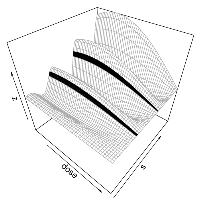
Figure 1: Example of the problem for a 2-dimensional surface. Here two dose-response curves (black lines), which are cross sections of a larger surface, are observed, and one is interested in this surface.

One may use a Gaussian process (GP, (Rasmussen and Williams, 2006) ) to characterize the entire $P+Q$ dimensional surface, but there are computational problems that make the use of a GP impractical. In the motivating example, there are over $4000$ unique $(s,d)$ pairs. GP regression requires inversion of the covariance matrix, which is inherently an $\mathcal{O}(n^{3})$ operation; inverting a $4000\times 4000$ matrix in each iteration of a Gibbs sampler is challenging, and, though the covariance matrix may be approximated leading to reduced computational burden (Quiñonero-Candela and Rasmussen (2005),Banerjee et al. (2013)), it is the author’s experience that, in the higher dimensional case of the data example, such approximations became accurate when the dimension of the approximation matrix approaches that of the matrix it is approximating. This leads to minimal computational savings. Further, if the approximation approach can be used resulting in computational benefits, the the proposed method can be used in in conjunction with such approximations.

As an alternative to GPs, one can use tensor product splines (de Boor (2000), Chapter 17); however, even if one defines a functional basis having only two basis functions for each dimension, the resulting tensor spline basis would have dimension $2^{P+Q},$ which is often computationally intractable. The proposed model sidesteps these issues by defining a tensor product of learned multi-dimsensional surfaces defined on $\mathcal{S}$ and $\mathcal{D}.$

One could consider the problem from a functional data perspective (Ramsay, 2006; Morris, 2015) by assuming a functional response over $\mathcal{S}\times\mathcal{D}.$ Approaches such as the functional linear array model (Brockhaus et al., 2015) and functional additive mixed models (Scheipl et al., 2015) are closest to the proposed approach as they allow the surface to be modeled as a basis defined on the entire space. For high dimensional spaces where interactions are appropriate, these approaches suffer the drawbacks because they do not allow for interactions in all dimensions. Additionally, these approaches assume that for any two observations $i,i^{\prime}$ when $s_{i}=s_{i^{\prime}}$, loadings are drawn from a distribution independent of $s_{i}.$ This differs from the proposed approach assumes, which correlates loadings through $\mathcal{S}.$

Clustering the functional responses is also a possibility. Here, one would model the surface using $\mathcal{D}$ and cluster using $\mathcal{S}.$ There are many functional clustering approaches (see for example Hall et al. (2001), Ferraty and Vieu (2006),Zhang and Li (2010),Sprechmann and Sapiro (2010) Delaigle and Hall (2012), Delaigle and Hall (2013), and references therein), but these methods predict $s\in\mathcal{S}$ based upon observing the functional response $f(d)$, which is the opposite of the problem at hand. In this problem, one observes information on the group (i.e., $s$) and one wishes to estimate the new response (i.e., $h(s,d)$). However different, such approaches can be seen as motivating the proposed method. Instead of clustering the loadings, the proposed approach assumes these loading for each basis is a value on a continuous function over $\mathcal{S}.$ This is similar to clustering as similarity is induced for any two responses having values in $\mathcal{S}$ that are sufficiently close.

As the number of basis functions used in the model is choice that may impact the model’s ability to represent an arbitrary surface, a sufficiently large number of basis functions are included. Parsimony in this basis set is ensured by adapting to the number components in the model using the multiplicative gamma prior (Bhattacharya and Dunson, 2011). This is a global shrinkage prior is used to remove components from the sum by stochastically decreasing the prior variance of consecutive loadings in the sum to zero. The sum adapts to the actual number of basis functions needed to model the data and the choice in the number of basis functions is less important as long as the number is sufficiently large.

In what follows, section 2 defines the model. Section $3$ gives the data model for normal responses and outlines a sampling algorithm. Section 4 shows through a simulation study the method outperforms many traditional machine learning approaches, and section $5$ is a data example applying the method to data from the US EPA’s ToxCast database.

2 Model

2.1 Basic Approach

Consider modeling the surface $h:(\mathcal{S}\times\mathcal{D})\rightarrow\mathbb{R}$ where $\mathcal{S}\subset\mathbb{R}^{P},$ $P\geq 1,$ and $\mathcal{D}\subset\mathbb{R}^{Q},$ $Q\geq 1$. Given $s\in\mathcal{S}$ and $d\in\mathcal{D},$ tensor product spline approaches (de Boor, 2000, chapter 17) approximate $h$ as a product of spline functions defined over $\mathcal{S}$ and $\mathcal{D},$ i.e.,

$$g\otimes f =g(s)f(d)\hskip 28.45274pt\forall s\in\mathcal{S},d\in\mathcal{D},$$ (1)

for $g:\mathcal{S}\rightarrow\mathbb{R}^{P}$ and $f:\mathcal{D}\rightarrow\mathbb{R}^{Q}.$ The tensor product spline defines $g$ and $f$ to be in the span of a spline basis. Assuming $g$ and $f$ are functions defined as

$$g(s) =\sum_{j=1}^{J}\lambda_{j}\phi_{j}(s)$$

and

$$f(d) =\sum_{l=1}^{L}\gamma_{l}\nu_{l}(d),$$

where $\{\phi_{j}(s)\}_{j=1}^{J}$ and $\{\nu_{j}(d)\}_{l=1}^{L}$ are spline bases. The tensor product spline is

$$g\otimes f=\sum_{j=1}^{J}\sum_{l=1}^{L}\rho_{jl}\phi_{j}(s)\nu_{l}(d),$$

where $\rho_{jl}=\lambda_{j}\gamma_{l}.$ As this approach typically uses 1- or 2-dimensional spline bases, when the dimension of $(\mathcal{S}\times\mathcal{D})$ is large the tensor product becomes impractical as the number of functions in the tensor product increases exponentially.

Where tensor product spline models define the basis through a spline basis a priori, many functional data approaches (e.g, Montagna et al. (2012)) model functions from a basis learned from the data. Often the function space is not defined over $(\mathcal{S}\times\mathcal{D})$ directly, but is constructed on a smaller dimensional subspace, defined to be $\mathcal{D}$ in the present discussion. For cross section $i,$ this approach models $h(s_{i},d),$ to be in the span of a finite basis $\{f_{1}(d),\ldots,f_{K}(d)\}.$ That is,

$$h(s_{i},d)=\sum_{k=1}^{K}z_{ik}f_{k}(d),$$ (2)

where $(z_{i1},\ldots,z_{iK})^{\prime}$ is a vector of basis coefficients. This effectively ignores $\mathcal{S}$ which may not be reasonable in many applications.

To model $h(s,d)$ over $(\mathcal{S}\times\mathcal{D}),$ the functional data and tensor product approaches can be combined. The idea is to define a basis over $(\mathcal{S}\times\mathcal{D})$ where each basis function is the tensor product of two surfaces defined on $\mathcal{S}$ and $\mathcal{D}$ respectively. Extending (2), define $\{g_{1}(s),\ldots,g_{K}(s)\}$ to be surfaces on $\mathcal{S},$ and replace each $z_{ik}$ with $\zeta_{k}g_{k}(s_{i}).$ Now, loadings are continuous function indexed by $s$, and a new basis $\{g_{1}\otimes f_{1},\ldots,g_{K}\otimes f_{K}\}$ with

$$h(s,d) =\sum^{K}_{k=1}\zeta_{k}g_{k}(s)f_{k}(d).$$ (3)

As pointed out by a referee, an alternative way to look at (3) is that of an ensemble learner (Sollich and Krogh, 1996), which includes techniques such as bagging Breiman (1996) and random forests (Breiman, 2001). Ensemble learners describe the estimate as a weighted sum of learners (see Murphy (2012) and references therein). In this way, model (3) can be looked as a weighted sum over tensor tensor product learners, and related to an ensemble based approach.

To define a tensor product, the functions $\{g_{k}(s)\}_{k=1}^{K}$ and $\{f_{k}(d)\}_{k=1}^{K}$ must be in of a linear function space (DeBoor, 2001, pg 293). For flexibility, let

$$g_{k} \sim\mathcal{GP}(0,\sigma^{g}_{k}(\cdot,\cdot))$$

$$f_{k} \sim\mathcal{GP}(0,\sigma^{f}_{k}(\cdot,\cdot))$$

where $\sigma^{g}_{k}(\cdot,\cdot)$ and $\sigma^{f}_{k}(\cdot,\cdot)$ are positive definite kernel functions. This places $g_{k}$ and $f_{k},$ $k=1,\ldots,K,$ in a reproducing kernel Hilbert space defined by $\sigma^{g}_{k}(\cdot,\cdot)$ or $\sigma^{f}_{k}(\cdot,\cdot),$ and embeds $h(s,d)$ in a linear space defined by the tensor product of these functions. By estimating the hyperparameters, this approach learns the basis of each function in (3), which may be preferable to a tensor spline approach that defines the basis a priori.

One may mistake this definition to be a GP defined by the tensor product of covariance kernels (e.g., see Bonilla et al. (2007)). Such an approach forms a new covariance kernel over $(\mathcal{S}\times\mathcal{D})$ as a product of individual covariance kernels defined on $\mathcal{S}$ and $\mathcal{D}$. For the proposed model, the product is the modeled function and not the individual covariance kernels.

2.2 Selection of K

The number of elements in the basis is determined by $K.$ The larger $K$, the richer the class of functions the model can entertain. In many cases, one would not expect a large number of functions to contribute to the surface and would prefer as few components as possible. One could place a prior on $K,$ but it is difficult to find efficient sampling algorithms in this case. As an alternative, the multiplicative gamma process (Bhattacharya and Dunson, 2011) is used to define a prior over the $\zeta_{1},\ldots\zeta_{k}$ that allows the sum to adapt to the necessary number of components. Here,

$$\zeta_{k}\sim N\bigg{(}0,\bigg{[}\phi\prod_{j=1}^{k}\delta_{j}\bigg{]}^{-1}\bigg{)}$$

with $\phi\sim\text{Ga}(1,1)$ and $\delta_{j}\sim\text{Ga}(a_{1},1),$ $1\leq j\leq K.$ This is an adaptive shrinkage prior over the functions. If $a_{1}>1,$ the variances are stochastically decreasing favoring more shrinkage as $k$ increases. The choice of this prior implies the surface defined by $\zeta_{k}g_{k}(s)f_{k}(d)$ is increasingly close to zero as $k$ increases. As many of the basis functions contribute negligibly to modeling the surface, this induces effective basis selection.

2.3 Relationships to other Models

Though GPs are used in the specification of the model, one may use alternative approaches such as polynomial spline models or process-convolution approaches (Higdon, 2002). Depending on the choice (3) can degenerate into other methods. For example, if $\sigma_{1}^{g},\ldots,$ and $\sigma_{K}^{g}$ are defined as white noise processes and $f_{1}(s),\cdots,$ and $f_{k}(s)$ defined to be in the linear span of the same finite basis, the model is identical to the approach of Montagna et al. (2012), which connects the model to functional data approaches. In this way, the additive adaptive tensor product model can be looked at as a functional model with loadings correlated by a continuous stochastic process over $\mathcal{S},$ instead of a white noise process.

If $P+Q=2$ and the functions $g_{1}$ and $f_{1}$ are defined using a spline basis, this approach trivially degenerates to the tensor product spline model. Similarly, let each function in $\{f_{1}(d),\ldots,f_{k}(d)\}$ be defined using a common basis, with,

$$f_{k}(d)=\sum_{\ell=1}^{L}\beta_{\ell}\phi_{\ell}(d),$$

where $\{\phi_{\ell}(d)\}_{\ell=1}^{L}$ is a basis used for all $f_{k}(d)$. In this case, model (3) can be re-written as

$$g(s,d)=\sum_{k=1}^{K}\sum_{\ell=1}^{L}\zeta_{k}\beta_{\ell}g_{k}(s)\phi_{\ell}(d).$$

Letting $\beta^{\ast}_{lk}=\zeta_{k}\beta_{\ell}$, one arrives at a tensor product model with learned basis $\{g_{1}(s),\ldots,g_{K}(s)\}$ and specified basis $\{\phi_{\ell}(d)\}_{\ell=1}^{L}.$

2.4 Computational Benefits

When $\mathcal{D}$ is observed on a fixed number of points and $s$ is the same for each cross section, the proposed approach can deliver substantial reductions in the computational resources needed when compared to GP regression. Let $r$ be the number of unique replicates on $\mathcal{D},$ and let $n$ be the total number of observed cross sections. For a GP, the dimension of the corresponding covariance matrix is $rn.$ Inverting this matrix is an $\mathcal{O}([rn]^{3})$ operation. For the proposed approach, there are $K$ inversions of a matrix of dimension $r$ and $K$ inversions of a matrix of dimension $n.$ This results in a computational complexity of $\mathcal{O}(K[r^{3}+n^{3}]),$ which can be significantly less than a GP based method. In the data example this results in approximately $1/20th$ the resources needed as compared to the GP approach, here $K=15$, $n=669$, and $r=7$. Savings increase as the experiment becomes more balanced. For example, if $n=r$ and there are the same number of observations as in the data example, then a GP approach would require $10,000$ times more computing time than the proposed method.

3 Data Model and Sampling Algorithm

3.1 Data Model

A Markov chain Monte Carlo (MCMC) sampling approach is outlined for normal errors. Assume that for cross section $i,$ $i=1,\ldots,n,$ one observes $C_{i}$ measurements at $\{(s_{i},d_{ic})\}_{c=1}^{C_{i}}.$ For error prone observation $y_{i}(s_{i},d_{ic}),$ let

$$y_{i}(s_{i},d_{ic})=h(s_{i},d_{ic})+\epsilon_{ic},$$

where $\epsilon_{ic}\sim N(0,\tau^{-1}).$ Define $N=\sum_{i=1}^{n}C_{i}.$ Model (3) assumes the surface is centered at zero; here, let the model be centered at $f_{0}(d).$

In defining $h_{k}(s)$ and $f_{k}(d)$, the covariance kernel, along with its hyper-parameters, determines the smoothness of the function. The squared exponential kernel is used to model smooth response surfaces. Let

$$\sigma^{g}_{k}(s,s^{\prime})=\varsigma_{k}\exp\bigg{(}-\theta_{k}\|s-s^{\prime}\|^{2}\bigg{)}$$ (4)

and

$$\sigma^{f}_{k}(d,d^{\prime})=\exp\bigg{(}-\omega_{k}\|d-d^{\prime}\|^{2}\bigg{)},$$ (5)

where $\|\cdot\|$ is the Euclidean norm, $\varsigma_{k}$ is the prior variance, $\theta_{k}$ and $\omega_{k}$ are scale parameters, and $1\leq k\leq K$. In this specification, the parameter $\zeta_{k}$ is not necessary; it is equivently defined through the variance of the GP where $\varsigma_{k}=(\phi\prod_{j=1}^{k}\delta_{j})^{-1}.$ To allow for a variance other than one for the process $f_{0}$, let $\sigma^{f}_{0}(d,d^{\prime})=\nu\exp(-\omega_{0}\|d-d^{\prime}\|^{2}).$

Depending on the application any positive definite kernel may be used. For example, one may wish to use a Matern kernel, which is frequently used in spatial statistics. As $\mathcal{S}$ is described in the application as the distance between spatial locations in an abstract chemical space, such an approach may be appropriate. Inpreliminary tests, a Matern kernel provides results that are qualitatively identical to the squared exponential kernel, and it is not considered further.

Given these choices the data model is

$$h(s,d) =f_{0}(d)+\sum^{K}_{k=1}g_{k}(s)f_{k}(d).$$ (6)

Appropriate priors are placed over the hyperparameters of $\{\sigma_{k}^{f}\}_{k=0}^{K}$ and $\{\sigma_{k}^{g}\}_{k=1}^{K}.$ For the length parameter of the squared exponential kernels in (4) and (5), uniform distributions, i.e., $\text{Unif}(a,b),$ $0<a<b,$ are placed over the scale parameters $\theta_{k}$ and $\omega_{k}.$ This places equal prior probability over a range of plausible values allowing the smoothness of the constituent basis to be learned. The value $a$ is chosen so that correlations between any two points in the space of interest are close to $1,$ and $b$ is chosen so that correlation between any two points in the resultant correlation is approximately to $0.$

3.2 Sampling Algorithm

Define the vector of observations $Y=\{y_{1}(s_{1},d_{11}),\ldots,y_{1}(s_{1},d_{1C_{1}}),$ $\ldots,y_{1}(s_{n},d_{n1}),$$\ldots,y_{1}(s_{1},d_{nC_{n}})\}^{\prime}$ to be the $(N\times 1)$ vector of measurements across the $n$ observed curves. Likewise define

$$\mathbf{G} =\left[\begin{array}[]{ccccc}1&g_{1}(s_{1})&g_{2}(s_{1})&\cdots&g_{K}(s_{1})\\ \vdots&\vdots&\vdots&&\vdots\\ 1&g_{1}(s_{1})&g_{2}(s_{1})&\cdots&g_{K}(s_{1})\\ \vdots&\vdots&\vdots&&\vdots\\ 1&g_{1}(s_{n})&g_{2}(s_{n})&\cdots&g_{K}(s_{n})\\ \vdots&\vdots&\vdots&&\vdots\\ 1&g_{1}(s_{n})&g_{2}(s_{n})&\cdots&g_{K}(s_{n})\\ \end{array}\right],$$

to be an $(N\times K+1)$ matrix, where each row corresponds to the loadings for observation $y_{i}(s_{i},d_{ic}).$ Let

$$\mathbf{F}=\left[\begin{array}[]{cccc}f_{0}(d_{11})&f_{1}(d_{11})&\cdots&f_{K}(d_{11})\\ \vdots&\vdots&&\vdots\\ f_{0}(d_{1C_{1}})&f_{1}(d_{1C_{1}})&\cdots&f_{K}(d_{1C_{1}})\\ \vdots&\vdots&&\vdots\\ f_{0}(d_{n1})&f_{1}(d_{n1})&\cdots&f_{K}(d_{n1})\\ \vdots&\vdots&&\vdots\\ f_{0}(d_{nC_{n}})&f_{1}(d_{nC_{n}})&\cdots&f_{K}(d_{nC_{n}})\\ \end{array}\right]$$

be an $(N\times K+1)$ matrix, where each row represents the basis functions evaluated at $d_{ic}.$ Using these definitions, (6) is expressible as

$$Y=\bigg{(}\mathbf{G}\circ\mathbf{F}\bigg{)}J^{\prime}+\mathbf{\epsilon},$$ (7)

where $\circ$ is the Schur product, $J=(1,1,\ldots,1)$ is a $K+1$ row vector, and $\mathbf{\epsilon}=(\epsilon_{11},\ldots,\epsilon_{iC_{1}},$ $\ldots,\epsilon_{n1},\ldots,\epsilon_{nC_{n}})^{\prime}$ is the $(N\times 1)$ vector of error terms.

Let $D=\{d^{\ast}_{r}\}_{r=1}^{R}$ be the set of $R$ uniquely observed inputs across all observations, and define $\mathcal{I}^{f}$ to be an $(N\times R)$ matrix where the rows corresponds to each element in $Y.$ For each row in $\mathcal{I}^{f}$, all entries are set to zero except at column $r.$ This entry is set to one, and it corresponds to the observation $y_{i}(s_{i},d_{ic})$ such that $d^{\ast}_{r}=d_{ic}.$ Likewise, define the matrix $\mathcal{I}^{g}$ to be an $(N\times n)$ matrix. For each row $r$, each entry is set to zero except at column $i,$ which is set to one. This entry corresponds to $Y_{r}=y_{i}(s_{i},d_{ic}).$

Sample from $\{g_{k}\}_{k=1}^{K},$ $\{f_{k}\}_{k=0}^{K},$ $\phi$, and $\{\delta_{k}\}_{k=1}^{K}$ in a series of Gibbs steps as follows:

1. For each $k$, $0\leq k\leq K$ , letting $Y^{\ast}=Y-(\mathbf{G}_{-k}\circ\mathbf{F}_{-k})J^{\prime}_{-k},$ where $G_{-k},$ $F_{-k},$ and $J_{-k}$ are $G,$ $F$ and $J$ without column $k,$ sample $f_{k}\sim N(M,V)$ at $\{d^{\ast}_{r}\}_{r=1}^{R}.$ Here

   $$V =\Sigma_{k}(\tau\mathcal{G}^{\prime}\mathcal{G}\Sigma_{k}+I)^{-1},$$

   $$M =V(\tau\mathcal{G}Y^{\ast}),$$

   were $\Sigma_{k}$ is the $(R\times R)$ covariance function constructed from $\sigma^{f}_{k}(\cdot,\cdot),$ $\mathcal{G}$ is an $(N\times R)$ matrix defined as $G_{k}\circ\mathcal{I}^{f},$ and $I$ is an $R\times R$ identity matrix.

2. For each $k$, $1\leq k\leq K$ and letting $Y^{\ast}=Y-(\mathbf{G}_{-k}\circ\mathbf{F}_{-k})J^{\prime}_{-k}$, sample $g_{k}\sim N(M,V)$ at $\{s_{i}\}_{i=1}^{n}.$ Here

   $$V =\Sigma_{k}(\tau\mathcal{F}^{\prime}\mathcal{F}\Sigma_{k}+I)^{-1},$$

   $$M =V(\tau\mathcal{F}^{\prime}Y^{\ast}),$$

   where $\Sigma_{k}$ is the $(n\times n)$ covariance matrix formed from $\sigma^{g}_{k}(\cdot,\cdot)$, $\mathcal{F}$ is an $(N\times n)$ matrix defined to be $(FJ^{\prime})\circ\mathcal{I}^{g},$ and $I$ is the $n\times n$ identity matrix.

3. Sample $\phi\sim\mbox{Ga}(c,d)$, where

   $$c =K\frac{n}{2}+a_{1},$$

   $$d =\bigg{[}\sum_{i=1}^{K}\bigg{(}\prod_{j=1}^{i}\delta_{j}\bigg{)}G_{i}^{{}^{\prime}}\Sigma_{i}G_{i}\bigg{]}+1,$$

   $G_{i}$ is a column vector from column $k$ of $G,$ and $\Sigma_{i}$ is the matrix formed from $\exp(-\theta_{i}||s-s^{\prime}||^{2})$

4. For each $k$ sample $\delta_{k}\sim\mbox{Ga}(c,d),$ where

   $$c =(K-k+1)\frac{n}{2}+a_{1}$$

   $$d =\bigg{[}\sum_{i=k}^{K}\phi\bigg{(}\prod_{j=1,j\neq k}^{i}\delta_{j}\bigg{)}G_{i}^{{}^{\prime}}\Sigma_{i}G_{i}\bigg{]}+1$$

   $G_{i}$ is a column vector from column $i$ of $G,$ $\Sigma_{i}$ is the matrix formed from $\exp(-\theta_{i}||s-s^{\prime}||^{2}),$ and $\bigg{(}\prod_{j=1,j\neq 1}^{1}\delta_{j}\bigg{)}=1$.

The other parameters in the model are sampled using Gibbs or Metropolis steps. The algorithm is written in the R programming language (R Core Team, 2015) using the Rcpp C++ extensions (Eddelbuettel, 2013) and the RcppArmadillo (Eddelbuettel and Sanderson, 2014) linear algebra extensions and is available in the supplement.

When the number of unique observations is small, it is possible to develop a block Gibbs sampler for all of the $\{f_{k}\}_{k=0}^{K}$ and $\{g_{k}\}_{k=1}^{K}.$ In large problems, this requires the inversion of a large matrix offsetting the benefits of the increased computational efficiency.

3.3 Predictive Inference

The posterior predictive distribution of $n^{\ast}$ unobserved cross sections of $h(s,d)$ at $\grave{S}=\{\grave{s}_{1},\ldots,\grave{s}_{n^{\ast}}\}$ is estimated through MCMC. Let the vector $g_{k}=(g_{k}(s_{1}),\ldots,g_{k}(s_{n}))^{\prime}$ be observed at $S=(s_{1},\ldots,s_{n})^{\prime}$ and one is interested in $\grave{g}_{k}=(g_{k}(\grave{s}_{1}),\ldots,g_{k}(\grave{s}_{n^{\ast}}))$ evaluated at $\grave{S}$; $g_{k}$ and $\grave{g}_{k}$ are jointly distributed as

$$\left[\begin{array}[]{c}g_{k}\\ \grave{g}_{k}\end{array}\right]\sim N\left(0,\left[\begin{array}[]{cc}\Sigma^{g}_{k}(S,S)&\Sigma^{g}_{k}(S,\grave{S})\\ \Sigma^{g}_{k}(\grave{S},S)&\Sigma^{g}_{k}(\grave{S},\grave{S})\end{array}\right]\right).$$

Here $\Sigma^{g}_{k}(S,S),$ $\Sigma^{g}_{k}(\grave{S},\grave{S}),$ $\Sigma^{g}_{k}(\grave{S},S)$ and $\Sigma^{g}_{k}(S,\grave{S})$ represent covariance matrices given $S,$ $\grave{S}$ and $\sigma^{g}_{k}(\cdot,\cdot).$ Using properties of the multivariate normal distribution, conditionally on $g_{k}$

$$\grave{g}_{k}\mid g_{k}\sim N\bigg{[}\Sigma^{g}_{k}(\grave{S},S)\Sigma^{g}_{k}(S,S)^{-1}g_{k},\Sigma^{g}_{k}(\grave{S},\grave{S})$$

$$-\Sigma^{g}_{k}(\grave{S},S)\Sigma^{g}_{k}(S,S)^{-1}\Sigma^{g}_{k}(S,\grave{S})\bigg{]}.$$

For each iteration, this expression is used to draw $\{\grave{g}_{1},\ldots,\grave{g}_{K}\}.$ Given this draw, as well as $\{f_{0},\ldots,f_{K}\}$ which represents $f_{0}(d),f_{1}(d)$ etc., evaluated at $D=\{d^{\ast}_{r}\}_{r=1}^{R}$, one can estimate the posterior predicted distribution of $h(\grave{S},D).$ If new $\grave{D}$ are of interest, the same technique can be applied to estimating $\{\grave{f}_{0},\ldots,\grave{f}_{K}.$ These values can be used with $\{\grave{g}_{k}\}_{k=1}^{K}$ to provide estimates for $h(\grave{S},\grave{D}).$

4 Simulation

This approach was tested on synthetic data. Here the dimension of $\mathcal{S}$ was chosen to be 2 or 3, and for a given dimension, $50$ synthetic data sets were created, For each data set, a total of $1000$ cross sections of $h(s,d)$ were observed at seven dose groups. Each data set contained a total of $7000$ observations.

To create a data set, the chemical information vector $s_{i}$, for chemical $i=1,\ldots,1000$, was sampled uniformly over the unit square/cube. At each $s_{i},$ $h(s_{i},d)$ was sampled at $d=0,0.375,0.75,1.5,3.0,4.5,$ and $6,$ from

$$h(s_{i},d)=\frac{\nu(s_{i})d^{m}}{\kappa(s_{i})^{m}+d^{m}},$$

where $\nu(s_{i})$ is the magnitude of the response and $\kappa(s_{i})$ is the dose $d$ where the response is at $50\%$ of the maximum. To vary the response over over $\mathcal{S},$ a different zero centered Gaussian process, $z(s)$, was sampled at $\{s_{i}\}_{i=1}^{1000},$ and for each simulation; $\nu(s_{i})$ and $\kappa(s_{i})$ were functions of $z(s)$ with $\nu(s_{i})=11\max(z(s_{i}),0)$ and $\kappa(s_{i})=\max(4.5-\nu(s_{i}),0).$ This resulted in the maximum response being between $0$ and approximately $50$ and the dose resulting in $50\%$ response being placed closer to zero for steeper dose-responses. Sample data sets used in the simulation are available in the supplement.

In specifying the model, priors were placed over parameters that reflect assumptions based upon the smoothness of the curve. For $\{\sigma_{k}^{g}(\cdot,\cdot)\}_{k=1}^{K},$ each $\theta_{k}$ was drawn from a discrete uniform distribution over the set $\{0.05,0.1,0.15,\ldots,4.05\}.$ Additionally, for $\{\sigma_{k}^{f}(\cdot,\cdot)\}_{k=0}^{K},$ each $\omega_{k}\sim\text{Unif}(0.1,1.5).$ For $\{\sigma_{k}^{g}(\cdot,\cdot)\}_{k=1}^{K}$, $\delta_{k}\sim\text{Ga}(2,1),$ $1\leq k\leq K$, which were the choices used in (Bhattacharya and Dunson, 2011). The choice of the parameters for the prior over the $\delta_{k}$ were examined, and the results were nearly identical with $\delta_{k}\sim\text{Ga}(5,1).$ The prior specification for the model was completed by letting $\tau\sim\text{Ga}(1,1).$

A total of $12,000$ MCMC samples were taken with the first $2,000$ disregarded as burn in. Trace plots from multiple chains were monitored for convergence. Convergence was fast usually occurring after $500$ iterations with approximately $4$ functions in the learned basis defining the surface (i.e. having posterior variance at or above 1).

To analyze the choice of $K$, the performance of the model was evaluated for $K=1,2,3$ and $15.$ The estimates produced from these models were compared against bagged multivariate adaptive regression splines (MARS) (Friedman, 1991) and bagged neural networks (Zhou et al., 2002) using the ‘caret’ package in R (from Jed Wing et al., 2016). Additionally, treed Gaussian Processes (Gramacy and Lee, 2008) ,using the R ‘tgp’ package (Gramacy et al., 2007), were used in the comparison. All packages were run using their default settings; $100$ bagged samples were used for both the MARS and neural network models. For the neural network model, $100$ hidden layers were used. Posterior predictions from the treed Gaussian process were obtained from the maximum a posteriori (MAP) estimate. This was done as initial tests revealed estimates sampled from the posterior distribution were no better than the MAP estimate, but sampling from the full posterior dramatically increased computation time making the full simulation impossible.

For each data set, $N=75,125,$ and $175$ curves were randomly sampled and used to train the respective model; the remaining curves were used as a hold out sample for posterior predictive inference with the true curve being compared against the predictions. All methods were compared using the mean squared predicted error (MSPE).

Table 1: Mean squared prediction error in the simulation of the adaptive tensor product approach for four values of K as well as treed Gaussian processes, bagged neural networks, and bagged multivariate regression splines (MARS).

		Adaptive TP
		K=1	K=2	K=3	K=15	Neural Net	MARS	Treed GP
2-dimensions	N=75	76.2	69.1	69.5	69.8	108.3	$215.2^{1}$	$839.7^{1}$
	N=125	56.9	48.5	48.8	48.7	92.4	205.8	$158.0^{1}$
	N=175	48.5	37.7	38.4	38.3	85.1	198.8	61.1
3-dimensions	N=75	164.9	162.0	155.4	155.4	185.2	$246.6^{1}$	$1521.5^{1}$
	N=125	128.6	125.0	121.0	121.0	160.4	223.4	$421.3^{1}$
	N=175	106.3	102.6	99.7	100.1	150.0	217.7	$163.5^{1}$
1 Trimmed mean used with $5\%$ of the upper and lower tails removed.

Table (1) describes the average mean squared predicted error across all simulations. For the adaptive tensor product model there is an improvement in prediction when increasing $K.$ For the 2-dimensional case the improvment occurs from $1$ to $2,$ but the results of $K=3$ and $15$ are almost identical to $K=2.$ For the 3-dimensional case, improvements are seen up to $K=3$ with identical results for $K=15$. These results support the assertion that one can make $K$ large and let the model adapt to the number of tensor products in the sum.

This table also gives the MSPE for the other methods. Compared to the other approaches, the adaptive tensor product approach is superior. For $N=175$, the treed Gaussian process, which is often the closest competitor, produces mean square prediction errors that are about $1.5$ times greater than the adaptive TP approach. For smaller values of $N,$ the treed GP as well as the bagged MARS approach failed to produce realistic predictions. In these cases, the trimmed mean with $5\%$ of the tails removed was used to provide a better estimate of center.

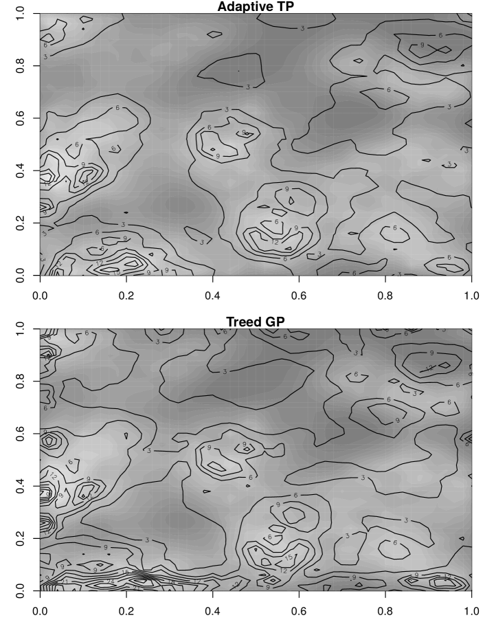
Figure 2: Comparison of the predictive performance between the adaptive tensor product and the treed Gaussian process. In the figure, the corresponding model’s root mean squared predicted error is given as a contour plot. The heat map represents the maximum dose response given the coordinate pair; lighter colors represent greater dose-response activity.

Figure (2), shows where the gains in prediction take place. As a surrogate for the intensity of the true dose-response function, the intensity of the dose-response at $d=6$ across $\mathcal{S}$ is shown in the 2-dimensional case. Dark gray regions are areas of little or no dose-response activity; lighter regions have the steeper dose-responses. Contour plots of the model’s root MSPE are overlaid on the heat maps. The top plot shows the performance of the adaptive TP and the bottom plot shows the performance of the treed GP, which was the closest competitor for this data set. The figure shows the adaptive TP is generally better at predicting the dose-response curve across $\mathcal{S}$ and that larger gains are made in regions of high dose response activity. This is most evident in the lower left corner of both plots, where regions of high dose response activity are located. At the peaks, the root MSPE is almost double that for the treed Gaussian process.

5 Data Example

The approach is applied to data released from Phase II of the ToxCast high throughput platform. The AttaGene PXR assay was chosen as it has the highest number of active dose-response curves across the chemicals tested. This assay targets the Preganene X receptor, which detects the presence of foreign substances and up regulates proteins involved with detoxification in the body; an increased response for this assay might relate to the relative toxicity of the given chemical.

Chemical descriptors were calculated using Mold² (Hong et al., 2008) where chemical structure was described from simplified molecular-input line-entry system (SMILES) information (Weininger, 1988). Mold² computes $777$ unique chemical descriptors. For the set of descriptors, a principal component analysis was performed across all chemicals. This is a standard technique in the QSAR liturature (Emmert-Streib et al., 2012, pg 44). Here, the first $38$ principal components, representing approximately $95\%$ of the descriptor variability, were used as a surrogate for the chemical descriptor $s_{i}$.

The database was restricted to $969$ chemicals having SMILES information available. In the assay, each chemical was tested across a range of doses between $0\hskip 2.0pt\mu M$ and $250\hskip 2.0pt\mu M$ with no tests done at exactly a zero dose. Eight doses were used per chemical, with each chemical being tested at different doses within the above range. Most chemicals had one observation per dose; however, some of the chemicals tested had multiple observations per dose. In total, the data set consisted of $9111$ data points from the $969$ distinct dose-response curves.

A random sample of $669$ chemicals was taken and the model wad trained to this data; in evaluating posterior predictive performance, the remaining $300$ chemicals were used as a hold out sample. In this analysis, $d$ was the log dose, where this value was rounded to two significant digits, and the same prior specification was in the simulation was used to train the model. To compare the prediction results, boosted MARS and neural networks were used; treed Gaussian processes were attempted, but the R package ‘tgp’ crashed after 8 hours during burn-in. The method of Low-Kam et al. (2015) was also attempted, but, the code was designed such that each chemical is tested at the same doses with the same number of replications per dose point. As the ToxCast data are not in this format, the method could not be applied to the data.

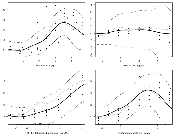
Figure 3: Four posterior predicted dose-response curves (black line) with corresponding $90\%$ predicted credible intervals (dotted lines) for four chemicals in the hold out samples having repeated measurements per dose. Grey dash-dotted line represents the predicted response from the bagged neural network.

Figures (3) and (4) show the posterior predicted curves (solid black line) with equal tail $90\%$ posterior predicted quantiles (dashed line) for eight chemicals in the hold out sample. Figure (3) describes the predictions for chemicals having multiple measurements per dose group, and figure (4) gives predictions having only a single observation per dose group. As compared to the observed data, these figures show the model provides accurate dose-response predictions across a variety of shapes and chemical profiles. Additionally the grey dashed-dotted line represents the prediction using the bagged neural network. These estimates are frequently less smooth and further off from the observed data than the adaptive tensor product splines. As additional confirmation the model is predicting dose-response curves based upon the chemical information, one can look a the chemicals from a biological mode of action perspective. For example in (3), it is interesting to note that the dose-response predictions for both Bisphenol A and $17\alpha$ Hydroxyprogesterone are similar, because both act similarly and are known to bind the estrogen receptor.

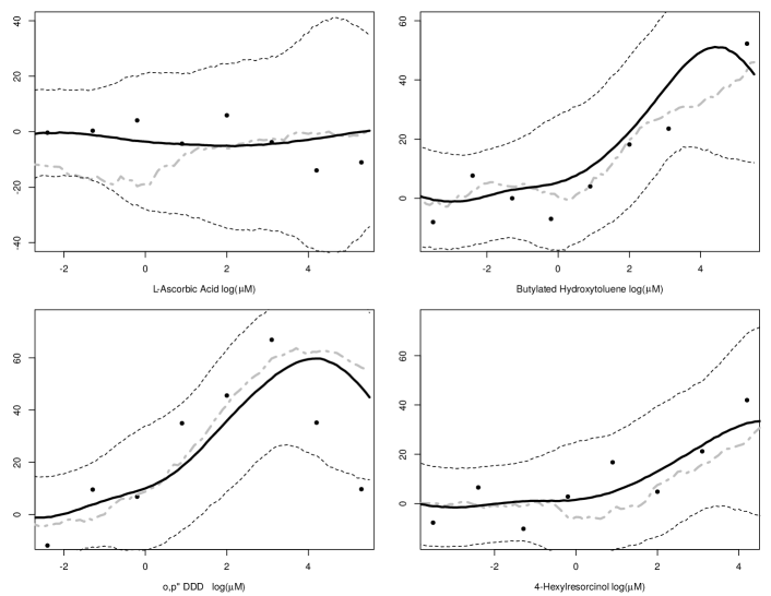
Figure 4: Four posterior predicted dose-response curves (black line) with corresponding $90\%$ predicted credible intervals (dotted lines) for four chemicals in the hold out samples having repeated measurements per dose. Grey dash-dotted line represents the predicted response from the bagged neural network.

In comparison to the other models, the adaptive tensor product approach also had the lowest predicted mean squared error and the predicted mean absolute error for the data in the hold out sample. Here the model had a predicted mean squared error of $342.1$ and mean absolute error of $11.7$, as compared to values of $354.7$ and $12.4$ for neural networks as well as $383.6$ and $13.4$ for MARS. These results are well in line with the simulation.

One can also compare the ability of the posterior predictive distribution to predict the observations in the hold out sample. To do this, lower and upper tail cut-points defined by $p$ were estimated from the posterior predictive distribution. The number of observations that were below the lower cut-point or above the upper cut-point were counted. Under the assumption the posterior predictive distribution adequately describes the data, this count is $\mbox{Binomial}(2p,n)$ where $n$ equal to the number of observations for that chemical. To test this assumption, the $90\%$ critical value was computed and compared to the count. This was done for $p=5,10$ and $15\%;$ here, $88,89,$ and $90\%$ of the posterior predictive distributions were at or below the $90\%$ critical value. This supports the assertion that the model is accurately predicting the dose-response relationship given the chemical descriptor information $\mathcal{S}$.

The method was also compared to standard QSAR approaches, which model a single data point. Similar to the standard QSAR methodology, a model was fit to each data-set $i$ and the response associated with a given dose was computed to be observation $y_{i}$. This value was then used in the model

$$y_{i}=x(s_{i})+\epsilon_{i},$$

where $x(s_{i})$ is a Gaussian process with squared exponential covariance kernel. The model was fit on the same $669$ observations in the training set and predictions were made of the response at that dose. Both this QSAR approach as well as the adaptive tensor product approach were compared to the hold out samples using the correlation coefficient, a standard practice in the QSAR literature. For the dose of $20\mu M$ the standard QSAR approach had a correlation of $0.42$ as compared to the co-mixture approaches’ correlation of $0.48.$ For the dose of $100\mu M$ a similar $0.06$ increase was seen, and, when observations that have a chemical within the training set defined as ‘close’ (i.e., a relative distance between two chemicals less than 2.2), this improvement in the correlation coefficient is almost $0.1$ (i.e, $0.5$ compared to $0.6$). This indicates that $10\%$ to $20\%$ improvements in the correlation coefficient using the proposed approach.

6 Conclusions

The proposed approach allows one to model higher dimensional surfaces as a sum of a learned basis, where the effective number of components in the basis adapts to the complexity of the surface. In the simulation and the motivating problem, this method is shown to be superior to competing approaches, and, given the design of the experiment, it is shown to require significantly less computational resources than GP approaches. Though this approach is demonstrated for high throughput data, it is anticipated it can be used for any multi-dimensional surface.

In terms of the application, this model shows that dose-response curves can be estimated from chemical SAR information, which is a step forward in QSAR modeling. Though such an advance is useful investigating toxic effects, it can also be used in therapeutic effects. It is conceivable, that such an approach can be used in silico to find chemicals that have certain therapeutic effects in certain pathways without eliciting toxic effects in other pathways. Such an approach may be of significant use in drug development as well as chemical toxicity research.

Future research may focus on extending this model to multi-output functional responses. For example, multiple biossays dose-responses may be observed, and, as they target similar pathways, are correlated. In such cases, it may be reasonable to assume their responses are both correlated to each other and related to the secondary input, which is the chemical used in the bioassay. Such an approach may allow for lower level in vitro bioassays, like the ToxCast endpoint studied here, to be used to model higher level in vivo responses.

References

- Banerjee et al. (2013) Banerjee, A., Dunson, D. B., and Tokdar, S. T. (2013). Efficient gaussian process regression for large datasets. Biometrika 100, 75.
- Bhattacharya and Dunson (2011) Bhattacharya, A. and Dunson, D. B. (2011). Sparse Bayesian infinite factor models. Biometrika 98, 291–306.
- Bonilla et al. (2007) Bonilla, E. V., Chai, K. M., and Williams, C. (2007). Multi-task Gaussian process prediction. In Platt, J., Koller, D., Singer, Y., and Roweiss, S., editors, Proc. of the 20th Annual Conference on Neural Information Processing Systems, pages 153–160. Neural Information Processing Systems Conference.
- Breiman (1996) Breiman, L. (1996). Bagging predictors. Machine learning 24, 123–140.
- Breiman (2001) Breiman, L. (2001). Random forests. Machine learning 45, 5–32.
- Brockhaus et al. (2015) Brockhaus, S., Scheipl, F., Hothorn, T., and Greven, S. (2015). The functional linear array model. Statistical Modelling 15, 279–300.
- Burden (2001) Burden, F. R. (2001). Quantitative structure-activity relationship studies using Gaussian processes. Journal of chemical information and computer sciences 41, 830–835.
- Czermiński et al. (2001) Czermiński, R., Yasri, A., and Hartsough, D. (2001). Use of support vector machine in pattern classification: Application to QSAR studies. Quantitative Structure-Activity Relationships 20, 227–240.
- de Boor (2000) de Boor, C. (2000). A practical guide to splines, Revised Edition, volume 27. Springer-Verlag.
- DeBoor (2001) DeBoor, C. (2001). A practical guide to splines. Springer.
- Deconinck et al. (2005) Deconinck, E., Hancock, T., Coomans, D., Massart, D., and Vander Heyden, Y. (2005). Classification of drugs in absorption classes using the classification and regression trees (CART) methodology. Journal of pharmaceutical and biomedical analysis 39, 91–103.
- Delaigle and Hall (2012) Delaigle, A. and Hall, P. (2012). Achieving near perfect classification for functional data. Journal of the Royal Statistical Society: Series B (Statistical Methodology) 74, 267–286.
- Delaigle and Hall (2013) Delaigle, A. and Hall, P. (2013). Classification using censored functional data. Journal of the American Statistical Association 108, 1269–1283.
- Devillers (1996) Devillers, J. (1996). Neural networks in QSAR and drug design. Academic Press.
- Eddelbuettel (2013) Eddelbuettel, D. (2013). Seamless R and C++ integration with Rcpp. Springer.
- Eddelbuettel and Sanderson (2014) Eddelbuettel, D. and Sanderson, C. (2014). RcppArmadillo: Accelerating R with high-performance C++ linear algebra. Computational Statistics and Data Analysis 71, 1054–1063.
- Emmert-Streib et al. (2012) Emmert-Streib, F., Dehmer, M., Varmuza, K., and Bonchev, D. (2012). Statistical modelling of molecular descriptors in QSAR/QSPR. John Wiley & Sons.
- Ferraty and Vieu (2006) Ferraty, F. and Vieu, P. (2006). Nonparametric functional data analysis: theory and practice. Springer Science & Business Media.
- Friedman (1991) Friedman, J. H. (1991). Multivariate adaptive regression splines. The annals of statistics pages 1–67.
- from Jed Wing et al. (2016) from Jed Wing, M. K. C., Weston, S., Williams, A., Keefer, C., Engelhardt, A., Cooper, T., Mayer, Z., Kenkel, B., the R Core Team, Benesty, M., Lescarbeau, R., Ziem, A., Scrucca, L., Tang, Y., Candan, C., and Hunt., T. (2016). caret: Classification and Regression Training. R package version 6.0-73.
- Gramacy et al. (2007) Gramacy, R. B. et al. (2007). tgp: an R package for Bayesian nonstationary, semiparametric nonlinear regression and design by treed Gaussian process models. Journal of Statistical Software 19, 6.
- Gramacy and Lee (2008) Gramacy, R. B. and Lee, H. K. H. (2008). Bayesian treed Gaussian process models with an application to computer modeling. Journal of the American Statistical Association 103, 1119–1130.
- Hall et al. (2001) Hall, P., Poskitt, D. S., and Presnell, B. (2001). A functional data-analytic approach to signal discrimination. Technometrics 43, 1–9.
- Higdon (2002) Higdon, D. (2002). Space and space-time modeling using process convolutions. In Anderson, C. W., Vic Barnett, P. C., Chatwin, P. C., and El-Shaarawi, A. H., editors, Quantitative methods for current environmental issues, pages 37–54. Springer.
- Hong et al. (2008) Hong, H., Xie, Q., Ge, W., Qian, F., Fang, H., Shi, L., Su, Z., Perkins, R., and Tong, W. (2008). MOLD2, molecular descriptors from 2D structures for chemoinformatics and toxicoinformatics. Journal of chemical information and modeling 48, 1337–1344.
- Judson et al. (2010) Judson, R. S., Houck, K. A., Kavlock, R. J., Knudsen, T. B., Martin, M. T., Mortensen, H. M., Reif, D. M., Rotroff, D. M., Shah, I., Richard, A. M., et al. (2010). In vitro screening of environmental chemicals for targeted testing prioritization: the ToxCast project. Environmental health perspectives 118, 485.
- Low-Kam et al. (2015) Low-Kam, C., Telesca, D., Ji, Z., Zhang, H., Xia, T., Zink, J. I., Nel, A. E., et al. (2015). A Bayesian regression tree approach to identify the effect of nanoparticles’ properties on toxicity profiles. The Annals of Applied Statistics 9, 383–401.
- Montagna et al. (2012) Montagna, S., Tokdar, S. T., Neelon, B., and Dunson, D. B. (2012). Bayesian latent factor regression for functional and longitudinal data. Biometrics 68, 1064–1073.
- Morris (2015) Morris, J. S. (2015). Functional regression. Annual Review of Statistics and Its Application 2, 321–359.
- Murphy (2012) Murphy, K. P. (2012). Machine learning: a probabilistic perspective. MIT press.
- Norinder (2003) Norinder, U. (2003). Support vector machine models in drug design: applications to drug transport processes and QSAR using simplex optimisations and variable selection. Neurocomputing 55, 337–346.
- Quiñonero-Candela and Rasmussen (2005) Quiñonero-Candela, J. and Rasmussen, C. E. (2005). A unifying view of sparse approximate Gaussian process regression. Journal of Machine Learning Research 6, 1939–1959.
- R Core Team (2015) R Core Team (2015). R: A Language and Environment for Statistical Computing. R Foundation for Statistical Computing, Vienna, Austria.
- Ramsay (2006) Ramsay, J. O. (2006). Functional data analysis. Wiley.
- Rasmussen and Williams (2006) Rasmussen, C. E. and Williams, C. K. (2006). Gaussian processes for machine learning. MIT Press.
- Roy et al. (2015) Roy, K., Kar, S., and Das, R. N. (2015). Understanding the basics of QSAR for applications in pharmaceutical sciences and risk assessment. Academic Press.
- Scheipl et al. (2015) Scheipl, F., Staicu, A.-M., and Greven, S. (2015). Functional additive mixed models. Journal of Computational and Graphical Statistics 24, 477–501.
- Sollich and Krogh (1996) Sollich, P. and Krogh, A. (1996). Learning with ensembles: How overfitting can be useful. Advances in neural information processing systems pages 190–196.
- Sprechmann and Sapiro (2010) Sprechmann, P. and Sapiro, G. (2010). Dictionary learning and sparse coding for unsupervised clustering. In Acoustics Speech and Signal Processing (ICASSP), 2010 IEEE International Conference on, pages 2042–2045. IEEE.
- Weininger (1988) Weininger, D. (1988). SMILES, a chemical language and information system: 1. introduction to methodology and encoding rules. Journal of chemical information and computer sciences 28, 31–36.
- Zhang and Li (2010) Zhang, Q. and Li, B. (2010). Discriminative K-SVD for dictionary learning in face recognition. In Computer Vision and Pattern Recognition (CVPR), 2010 IEEE Conference on, pages 2691–2698. IEEE.
- Zhou et al. (2002) Zhou, Z.-H., Wu, J., and Tang, W. (2002). Ensembling neural networks: many could be better than all. Artificial intelligence 137, 239–263.