Distributed deep learning on edge-devices:
feasibility via adaptive compression
Abstract
A large portion of data mining and analytic services use modern machine learning techniques, such as deep learning. The state-of-the-art results by deep learning come at the price of an intensive use of computing resources. The leading frameworks (e.g., TensorFlow) are executed on GPUs or on high-end servers in datacenters. On the other end, there is a proliferation of personal devices with possibly free CPU cycles; this can enable services to run in users’ homes, embedding machine learning operations. In this paper, we ask the following question: Is distributed deep learning computation on WAN connected devices feasible, in spite of the traffic caused by learning tasks? We show that such a setup rises some important challenges, most notably the ingress traffic that the servers hosting the up-to-date model have to sustain.
In order to reduce this stress, we propose AdaComp, a novel algorithm for compressing worker updates to the model on the server. Applicable to stochastic gradient descent based approaches, it combines efficient gradient selection and learning rate modulation. We then experiment and measure the impact of compression, device heterogeneity and reliability on the accuracy of learned models, with an emulator platform that embeds TensorFlow into Linux containers. We report a reduction of the total amount of data sent by workers to the server by two order of magnitude (e.g., -fold reduction for a convolutional network on the MNIST dataset), when compared to a standard asynchronous stochastic gradient descent, while preserving model accuracy.
I Introduction
Machine learning methods, and in particular deep learning, are nowadays key components for building efficient applications and services. Deep learning recently permitted significant improvements over state-of-the-art techniques for building classification models for instance [1]. Its use spans over a large spectrum of applications, from face recognition in [2], to natural language processing [3] and to video recommendation in YouTube [4].
Learning a model using a deep neural network (we denote DNN hereafter) requires a large amount of data, as the precision of that model directly depends on the quantity of examples it gets as input and the number of times it iterates over them. Typically, the last image recognition DNNs, such as [5] or [1], leverage very large datasets (like Imagenet [6]) during the learning phase; this leads to the processing of over TB of data. The direct consequence is the compute-intensive nature of running such approaches. The place of choice for running those methods is thus well provisioned datacenters, for the more intensive applications, or on dedicated and GPU-powered machines in other cases. In this context, recently introduced frameworks for learning models using DNNs are benchmarked in cloud environments (e.g., TensorFlow [7] with GPU-enabled servers and 16Gbps network ports).
Meanwhile, the number of processing devices at the edge of the Internet keeps increasing in a steep manner. In this paper, we explore the possibility of leveraging edge-devices for those intensive tasks. This new paradigm rises significant feasibility questions. The dominant parameter server computing model, introduced by Google in 2012 [8], uses a set of workers for parallel processing, while a few central servers (denoted the parameter server (PS) hereafter for simplicity) are managing shared states modified by those workers. Workers frequently fetch the up-to-date model from the PS, make computation over the data they host, and then return gradient updates to the PS. Since DNN models are large (from thousands to billions parameters [9]), placing those worker tasks over edge-devices imply significant updates transfer over the Internet. The PS being in a central location (typically at a cloud provider), the question of inbound traffic is also crucial for pricing our proposal. Model learning is facing other problems such as device crashes and worker asynchrony. We note that those concerns differ from federated optimization techniques [10], that aim at removing worker asynchrony to reach minimal communication, but at the cost of removing processing parallelism that motivated the PS approach in the first place.
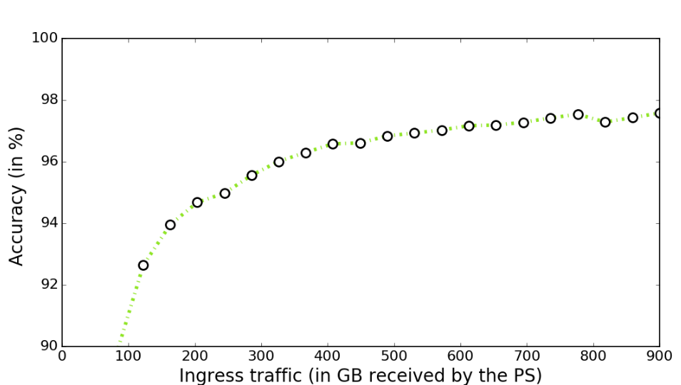
To illustrate the feasibility question, we implement the largest distribution scenario considered in the TensorFlow paper [7], where 200 machines are collaborating to learn a model. We measure the aggregated traffic at the PS generated by the learning of a classifier on the MNIST dataset, and plot it on Figure 1. We observe a considerable amount of ingress traffic received by the PS, of the order of Terabyte for an accurate model. This amount of traffic is due to workers sending their updates to the PS, and is not even reported in research studies, as well provisioned and dedicated data center networks are assumed. Clearly, in a setup leveraging edge-devices, this amount of ingress traffic has to be drastically reduced to remove weight on both the Internet and on the PS. Meanwhile, the data to be processed at edge-devices themselves is not the limiting factor (MB each in this experiment, as the dataset is split among workers). Our solution is to introduce a novel compression technique for sending updates from workers to the PS, using gradient selection [11]. We thus study the model accuracy with regards to update compression, as well as with regards to device reliability.
The main contributions of this paper are the following: 1) Exposing the parameter server model implications, in an edge-device setup. 2) Introducing AdaComp, a novel compression technique for reducing the ingress traffic at the PS. We detail AdaComp formally, and also open-source its code for public use.111The code is available on https://github.com/Hardy-c/AdaComp 3) Experimenting AdaComp within TensorFlow, and comparing it to competitors with regards to model accuracy.
First, in Section II, we briefly present the basics of deep learning, and of distributed learning in datacenters. Section III introduces the considered execution setup on edge-devices, and important performance metrics. Section IV presents AdaComp, before evaluating it and its competitors in Section V. We present related work in Section VI and concluding remarks in Section VII.
II Distributed Deep Learning
II-A Basics on DNN training on a single core
DNNs are machine learning models used for supervised or unsupervised tasks. They are composed of a large succession of layers. Each layer is the result of a non-linear transformation of the previous layer (or input data) given a weight matrix and a bias vector . In this paper, we focus on supervised learning, where a DNN is used to approximate a target function (e.g., a classification function for images).
For instance, given a training dataset of images and associated labels , a DNN has to adapt its parametric function , with a vector containing the set of all parameters, i.e., all entries of matrices and vectors . Training is performed by minimizing a loss function which represents how good is the DNN at approximating , given by :
| (1) |
where is the error of the DNN output for with parameters . The minimization of is performed by an iterative update process on the parameters called gradient descent (GD). At each step, the algorithm updates the parameters as follows (vector notations) :
| (2) |
with the learning rate and approximating the gradient of the error function. is computed by a back-propagation step [12] on at time . In the following sections, we use the more efficient variant of GD, called Stochastic Gradient Descent (SGD) [13], which processes a mini-batch of the training dataset per iteration.
II-B Distributed Stochastic Gradient Descent in the Parameter Server Model
To speed-up DNN training, Dean et al. proposed in [8] the parameter server model, as a way to distribute computation onto up to hundreds of machines. The principal idea is to parallelize data computation: each compute node (or worker) processes a subset of the training data asynchronously. For convenience, we report the core notations in Table I.
| PS | The parameter server, hosting the up-to-date |
| The number of workers (excluding the PS) | |
| The identifiers of the workers | |
| Size of mini-batches | |
| The model learning rate | |
| The compression ratio | |
| (% of selected parameters [per or ]) | |
| Training data local to a worker | |
| The number of performed iterations | |
| Vector containing all parameters at iteration ,i.e., all entries of matrices and vectors at | |
| The -th entry of | |
| Vector containing all updates to | |
| The global staleness of update | |
| Local update staleness, associated to parameter | |
| Local learning rate associated to given | |
| , and | The local parameter vector state at worker , the update computed from by worker and the resulting compressed update |
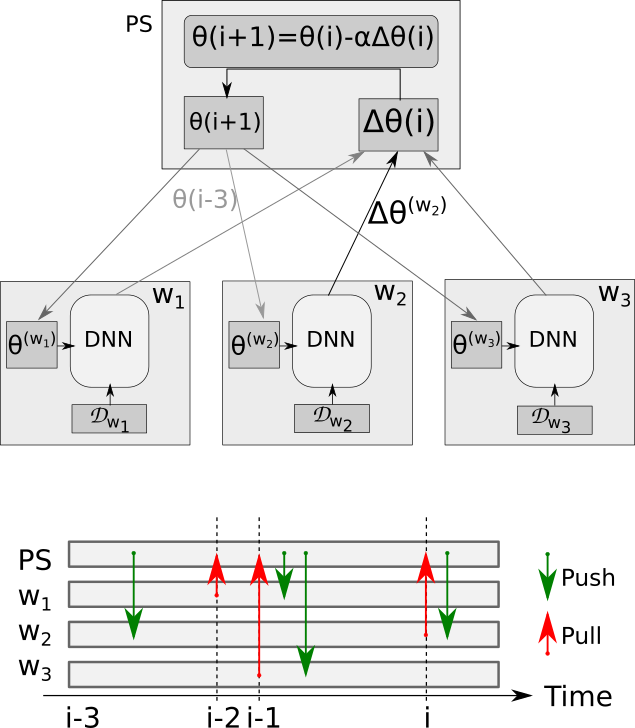
The parameter server model is depicted on Figure 2. In a nutshell, the PS starts by initializing the vector of parameters to learn, . Training data is split across workers . Each worker runs asynchronously, and whenever it is ready, takes the current version of the parameter vector from the PS, performs a SGD step and sends the vector update (that reflects the learning on its data) to the PS. In Figure 2, worker gets the state of at iteration , performs a SGD step and sends an update to the PS. Meanwhile, workers and , which finish their step before , send their updates. At each update reception, the PS updates , and increments the timestamp of (e.g., becomes after the reception of ’s update). An important parameter is the mini-batch size, denoted by , which corresponds to the subset size of the local data that each worker is computing upon, before sending one update to the PS (e.g., if , an update is sent by after its DNN has processed images of ).
Note that in the PS model, the fact that workers are training their local vector in parallel and then send the updates introduces concurrency, also known as staleness [14]. The staleness of the local vector for a worker is the number of times has evolved in between the fetch by , and the time where it itself pushes an update (e.g., on Figure 2, ’s update staleness is equal to ).
III Distributed Deep Learning on Edge-Devices
The execution setup we consider replaces the datacenter worker nodes by edge-device nodes (e.g., personal computers of volunteers with SETI@home, or home gateways [15]) and the datacenter network by the Internet. The PS remains at a central location. In this context, we assume that the training data reside with the workers; this serves for instance as a basis for privacy-preserving scenarios [11], where users have their photos at home, and want to contribute to the computing of a global photo classification model, but without sending their personal data to a cloud service.
The formal execution model remains identical to the PS model: we suppose that workers have enough memory to host a copy of , data is shuffled on the workers, and finally they agree to collaborate to the machine learning task (tolerance to malicious behaviours is out of the scope of this paper). The stringent aspect of our setup is the lower connectivity capacity of workers, and their expected smaller reliability [15]. Regarding connectivity, we have in mind a standard ASDL/cable setup where the bottleneck at the device is the uplink (with e.g., respectively 100Mb/10Mb for down/up bandwidth); we thus optimize on the worker upload capacity by compressing the updates it has to send i.e., the push operation, rather than the opposite i.e., the pull operation.
III-A Staleness mitigation
Asynchronous vector fetches and updates by workers involve perturbations on the SGD due to the staleness of local . The staleness, proportional to the number of workers (please refer to [16], [17] or [14] for in depth phenomenon explanation), is an important issue in asynchronous SGD in general. A high staleness has to be avoided, as workers that are relatively slow will contribute, through their update, to a that has evolved (possibly significantly) since they last fetched their copy of . This factor is known for slowing down the computation convergence [14]. In order to cope with it, works [18] and [14] adapt the learning rate as a function of the current staleness to reduce the impact of stale updates, which will also reduce the number of updates needed to train .
III-B Reducing ingress traffic at the PS
In the edge-device setting, where devices collaborate to the computation of a global , we argue that the critical metric is the bandwidth required by the PS to cope with incoming worker updates. This allows for frontend server/network dimensioning, and is also a crucial metric, as cloud providers often bill on upload capacities to cloud servers (see e.g., Amazon Kinesis, which charges depending on the number of 1MB/s message queues to align as frontends). Since our setup implies best effort computation at devices, not to saturate uplink, the workers are sending updates to the PS as background tasks. We thus measure the total ingress traffic at the PS collection point, in order to have an aggregated view of the upload traffic from workers, incurred by the deep learning tasks.
Compression
Shokri et al. [11] proposed a compression mechanism for reducing the size of the updates sent from each worker to the PS, named Selective Stochastic Gradient Descent. At the end of an iteration over its local data, a worker sends only a subset of computed gradients, rather than all of them. The selection is made either randomly, or by keeping only the largest gradients. The compression ratio is represented by fixed value . They experimentally show that model accuracy is not impacted much by this compression method for a SGD in a single core (with e.g., a MLP model accuracy decreasing from 98,10% to 97,07% accuracy, on the MNIST dataset and a selection of 1% of parameters per update).
In the light of this Section, the total amount of ingress traffic received at the PS is of the order of , with the size of (e.g., in MB). As the crucial focus of machine learning is the accuracy of the learned model, we have shown (Figure 1) that unfortunately it is not linear with the amount of data received at the PS. That is why we measure the accuracy/ingress traffic tradeoff experimentally, in the remaining of this paper. As we shall see in the evaluation Section, approach [11] in an edge-device setup manages to reduce the size of updates, but at the cost of accuracy. This is a clear impediment, because deep learning is leveraged for its state-of-art accuracy results. In order to cope with both ingress traffic and accuracy maintenance, we now introduce the AdaComp algorithm.
IV Compressed updates with AdaComp
AdaComp is a solution to conveniently combine the two concepts of compression and staleness mitigation, for further compressing worker results. This permits drastic ingress traffic reduction, for a comparable accuracy with best related work approaches.
Rationale
To do so, we propose the following approach. We first observe that the content of updates pushed by workers are often sparse (i.e., most of the parameters have not changed, for most of ): a selection method based on largest values of update is a good solution to compress it with little loss of information. Second, we observe that staleness mitigation is handled solely at the granularity of a whole update, in related approaches. From those remarks, we propose to compress updates pushed by worker and use staleness mitigation. The novelty in AdaComp is to compute staleness not on an update, but per parameter. Our intuition is that sparsity and staleness mitigation on individual parameters will allow for increased efficiency in asynchronous worker operation, by removing a significant part of update conflicts. An independent staleness score computed for each parameters is a reasonable assumption: F. Niu et al. [19] consider parameters as independent during the SGD.
Selection method
We propose a novel method for selecting gradient at each worker: only a fraction of the largest gradients per matrix and vector are kept. This selection permits to balance learning across DNN layers and better reflects computed gradients as compared to a random selection (or solely the largest ones across the whole model) as in [11].
Algorithm details
AdaComp operates in the following way, also described with pseudo-code in Algorithm 1 and 2. The PS keeps a trace of all received updates at given timestamps (as in [16, 14]). When a worker pulls , it receives the associated timestamp . It computes a SGD step and uses the selection method to compress the update. Meanwhile, intermediate updates (pushed by other workers) increase the timestamp of the PS to . Instead of computing the same staleness for each of the update , we define an adaptive staleness for each parameter as follows :
| (3) |
where is the indicator function of condition equal to if condition is true and otherwise. The staleness is then computed individually for each parameter by counting the number of updates applied on it since the last pull by the worker. We use the update equation inspired by [14]:
| (4) |
where
| (5) |
The is the learning rate computed for the -th parameter of given staleness . The parameter that was updated since the worker pull, will see reduced as a function of the staleness, as shown in equation (5). This method has the effect of reducing the concurrency between the possibly numerous asynchronous updates taking place along the learning task, while taking advantage of gradient selection to reduce update size222Please note that the best low level data representation for update encoding is out of the scope of this paper: it will causes at best a reduction of a small factor w.r.t. python serialization (i.e., the TensorFlow language), while we target in this paper two orders of magnitude decrease on the network footprint by targeting the algorithmic scope of distributed deep learning..
Complexity
AdaComp implies increased complexity for the PS to compute the adaptive staleness for each . In terms of memory, the PS has to maintain the last updates, where is the worst delay (i.e., the delay of the last worker which did not sent an update). Only indexes of non-zero parameters are maintained, leading to a memory complexity equals to . In the worth-case, the computation of requires dichotomous searches in lists of sizes (assuming that indexes of each update are stored in a sorted list). The computational complexity of is for a parameter, and this computation occurs for parameters at each iteration. We thus obtain an overall complexity of per iteration for the PS. Note that has the same magnitude as (see [14]), so we can rewrite the complexity as .
Note that in the classical PS model the computation complexity is ; we thus conclude in a computation complexity increase by in AdaComp, highlighting the proposed computation vs communication tradeoff. Finally for workers, the selection of the largest parameters does not increase the complexity.
V Experimental Evaluation
V-A Experimental platform
For assessing the value of AdaComp in a controlled and monitored environment, we choose to emulate the overall system on a single powerful server. The server allows us to remove the hardware and configuration constraints. We choose to represent edge-devices through Linux containers (LXC) on a Debian high end server (Intel(R) Xeon(R) CPU E5-2667 v3 @ 3.20GHz CPUs, a total of 32 cores, and 1/2TB of RAM). Each of them runs a TensorFlow session to train locally the DNN (we note that TensorFlow is also running in containers, while executed in a datacenter environment). The traffic between LXCs can then be managed by the host machine with virtual Ethernet (or veth) connections. We recall the open-sourcing of the algorithm code (please refer to footnote 1).
An experiment on this platform is as follows. A set of LXC containers is deployed, to represent the workers. Each worker in a container has access to a proportion of the training dataset. One LXC container is deployed to run the PS code. All workers are connected to PS by a veth virtual network. Finally, one last LXC container is deployed to evaluate the accuracy evolution of .
During the execution, the platform adds a random waiting time, for each worker, between the effective computation time and the push step to the PS. This time ensures that the order of worker updates is random, mimicking the possible variety in hardware or resource available to the workers (we furthermore conduct an experiment on this device heterogeneity in the experiment Section). We report a runtime of about day for each run (i.e., for reaching iterations).
In such a setup, the interesting metric to observe is the accuracy reached according the number of iterations performed, which is the same, whether computation takes place in an emulated setup or in a real deployment. The benefit of our platform is a tight monitoring of the resulting TCP traffic, during the learning task.
V-B Experimental setup and competitors
We experiment our setup with the MNIST dataset [20], also used by our competitor [11]. The goal is to build an image classifier able to recognize handwritten digits (i.e., 10 classes). The dataset is composed of a training dataset with images, i.e., per class, and a test dataset with images. Each image is represented by pixel with a 8-bit grey-level matrix.
We experiment in this paper on a Convolutional Neural Network (CNN), consisting of two convolutional layers and two full-connected layers ( parameters), and is taken from the Keras library [21] for the MNIST dataset. Our tech report [22] additionally contains experiments over a Multi-Layers Perceptron model. The experiments are launching workers, and one PS, corresponding to the scale of operation reported by TensorFlow [7].
We compare the performance of AdaComp to the ones of 1) the basic Async-SGD method (which we denote ASGD) [17] as a baseline. 2) the Comp-ASGD algorithm, which is similar to ASGD, but implements a gradient selection as described in [11]. For both competitors, the learning rate is divided by staleness and is global to each update.
V-C Accuracy results
All experiments are executed until the PS has received a total of updates from the workers; this corresponds to an upper bound for convergence of the best performing approaches we present in this Section. Experiments have been run 3 times; plots show average, minimal and maximal values of the moving average accuracies for each run. Final accuracy is the mean of the maximal accuracy reached by each run.
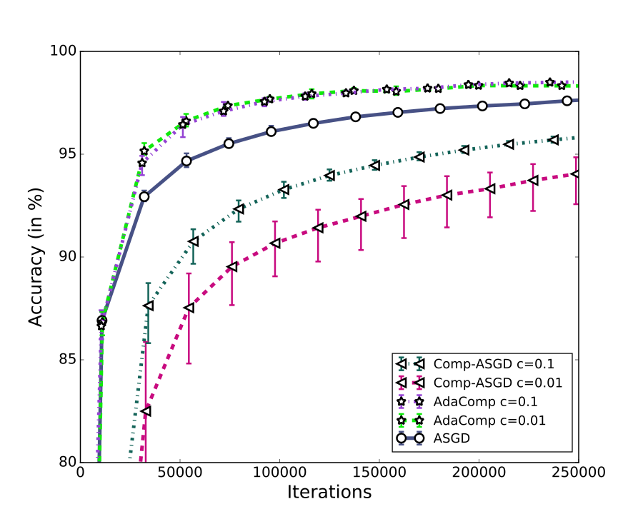
Figure 3 (left) plots the accuracy of the model depending on the number of iterations. Figure 3 (right) reports the accuracy as function of the ingress traffic, measured at the PS. ASGD, Comp-ASGD and AdaComp are experimented within the same setup with a batch size : . For both Comp-ASGD and AdaComp, we test the compression ratios and , respectively representing and of the local parameters sent as an update by a worker to the PS.
Figure 3 (left) first shows that compression affects Comp-ASGD results, while it does not prevent AdaComp to perform better than both ASGD and Comp-ASGD. Final accuracy results are for ASGD , for Comp-ASGD and ( and respectively), and finally for AdaComp and . We report in [22] that lower values for (equals to or ), result in degraded accuracy.
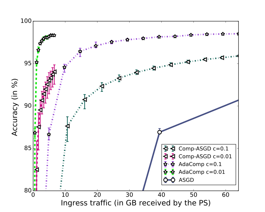
Regarding the resulting ingress traffic by considered algorithms, presented on Figure 3 (right), we observe striking differences. As expected, not relying on compression causes ASGD to produce a large amount of traffic in destination to the PS (up to GB after iterations), while the accuracy is still not at its possible best. The effect of compression for Comp-ASGD and AdaComp, with low values of , is clearly noticeable. This allows to drastically reduce the amount of traffic the PS has to deal with, and then in turn reduces the operational cost of the deep learning task.
As a mean for precise comparison, we fix an accuracy level of , and report the resulting aggregated ingress traffic for each algorithm. AdaComp generates GB of ingress traffic with , representing times less traffic than ASGD. Comp-ASGD does not manage to reach this accuracy level.
We conclude that AdaComp outperforms ASGD and Comp-ASGD on both accuracy and ingress traffic (consistently with the second model experimented in [22]). While compressing the size of updates naturally leads to a reduced ingress traffic at he PS, AdaComp beating ASGD is less intuitive: AdaComp counters the effect of staleness due to the asynchronous updates, by using fine grained updates. The probability of update conflicts of a parameter is indeed less important than at the level of the whole set of parameters in an update (as performed in Comp-ASGD). This allows for a higher learning rate for parameters not concerned by staleness. This makes it possible to consider DNN computation on edge-devices (e.g., for a home gateway connected 24/7, this experiment corresponds to an average of KB/s upload over a week).
V-D AdaComp accuracy facing worker failures
A key element for accuracy of distributed deep learning is the reliability of computation facing device failures. We then consider fail-stop type of failures for workers (e.g., they crash without warning messages or partial updates to the PS). In addition, we consider that the local data of a crashed node are lost for the system. We tune the probability that each worker crashes after each push operation. We then simply freeze the randomly selected containers, to emulate crashes. In expectation, half of the initial population of workers will have crashed by the end of the experiment (i.e., workers are present at , and only survived at ). Results for AdaComp with are presented on Table II. We operate on the MLP presented in our tech report [22].
The first observation, with AdaComp with crashes, is that crashes have very little effect on accuracy (, i.e., less). This is due to the fact that the MNIST dataset is ”too rich” for the learning task: this translates by nodes crashing with not mandatory data for the accuracy of in the end.
| Parameters | Reached accuracy | ||
|---|---|---|---|
| Training set | Crashes | n | |
| images | no | 200 | |
| images | yes | 200 | |
| images | no | 200 | |
| images | yes | 200 | |
| images | no | 100 | |
We run the same experiment with only of the original MNIST dataset as training set (i.e., images). We report a loss of accuracy of between AdaComp with crashes and AdaComp with no crashes (with for both), close to the previous loss of accuracy with the whole training dataset. To further explain this phenomenon, we run an experiment where only workers participate to the learning task. We test AdaComp for , , % of the training set and no crash (i.e., equivalent to a scenario where half of the 200 nodes would have disappeared with thus of data prior to the start of the learning task). Accuracy is , versus for the previous experiment with crashes. This underlines that the crashed nodes have in fact participated to some extent to the model learned (otherwise AdaComp with crashes and of training set would also have terminated around accuracy as well).
This experiment underlines that crash failures of edge-devices will not affect the accuracy of the model if the dataset over which they learn is rich enough, and that the impact of failures remains very limited otherwise (assuming little contribution of devices).
V-E AdaComp accuracy facing heterogeneous workers
For each edge-device, the joint effect of its network constraints, hardware and concurrently executed tasks could lead to significantly varying latencies in the computation of a batch. Distributed learning tasks then have to cope with that worker heterogeneity of completion times.
To assess the performance of AdaComp facing this heterogeneity, this experiment builds on three different classes of workers: a fast class, a medium and a slow one. Fast workers send 10 times more updates to the PS than medium workers, and 100 time more than slow workers. The proportion of workers in each class is respectively , and (workers do not switch class during runtime). We run AdaComp with parameters , . We experiment on a large training set, composed by the MNIST training dataset (i.e., with images) and a reduced training set composed by of the MNIST dataset (i.e., images).
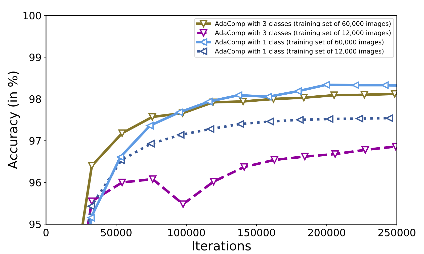
Figure 4 plots the accuracy of the model described in V-B (then with solely one class of workers) and with the three classes of workers. The first observation is that AdaComp with only one class of workers causes a higher final accuracy, as compared to three classes (respectively versus for the large training set and versus for the reduced training set). Note that the gap of accuracy is larger when the training set is reduced. Figure 4 shows that AdaComp with three classes of workers converges faster at the beginning than AdaComp with one class (experiment with large training set). This underlines that, with three classes, the fastest workers contribute more to the learning in a shorther amount of iterations, quickly increasing the accuracy at the beginning (with a low staleness score per update). However, when the DNN is adapted to the fastest workers updates, it does not then learn enough from slower workers to reach the same accuracy than the experiment with one class. This phenomenon is particularly salient on the reduced training set curves.
This experiment shows that distributed learning with heterogeneous workers, as expected in real deployments, is feasible as convergence occurs. It tends to reduce the contribution of the slowest workers as compared to that of the faster ones. Such as in the previous experiment with crash failures, the impact of heterogeneity on the final accuracy depends on the processed dataset (impact is reduced when using a richer training set).
VI Related Work
There are numerous alternatives to classical SGD to speed-up deep learning such as Momentum SGD [23], Adagrad [24], or Adam [25]. Those methods use adaptive gradient descent for each parameter, but are meant to run on a single machine (i.e., are not suitable for distributed computing), and then are not competing with AdaComp for parallel speed-up. Future works may adapt Adam with AdaComp to speed-up the learning in a distributed setup.
The parameter server model is popular for distributing SGD with e.g., DistBelief [8], Adam [26], and TensorFlow [7] as the principal ones. Increasing the number of workers in such an asynchronous environment causes staleness problems, that has been addressed either 1) algorithmically, or by means of 2) synchronization.
1) In [14], W. Zhang et al. propose to adapt the learning rate according to the staleness for each new update. The PS divides the learning rate by the computed staleness of the worker. This method limits the impact of highly stale updates. More recently, Odena [18] proposed to maintain the averaged variance of each parameters to precisely weight new updates. Combined with the previous method, this allows to adapt the learning rate for each parameter according the changes provided by previous workers. The learning rate will be higher for parameters which witnessed few changes than those which witnessed big changes during the last updates. This method is close to AdaComp, but does not take into account sparse updates.
2) A simple solution to avoid staleness problems is to synchronize worker updates. However, waiting for all workers at each iteration is time consuming. W. Zhang et al. [14] propose the -softSync protocol where the PS waits a fraction of all workers at each iteration before updating parameters. A more accurate gradient is computed by averaging the computed gradient of the fraction of workers. Another recent work of Chen et al. [27] shows that a synchronous SGD could be more efficient if the PS does not wait the last workers at each iteration. In our setup, workers are user-devices without any guarantee on the upper bound of their response time. This calls for efficient asynchronous methods like AdaComp.
Finally, at the other extreme of the parallelism versus communication tradeoff, so-called federated optimization has been introduced [10, 28, 29]. A model is learned given a very large number of edge-devices each only processing over a few data, and each being equipped with a poor connection. A subset of active workers (which changes at each iteration) runs many iterations over workers data before their model is shared. Global updates are then performed synchronously. Federated learning is thus communication-efficient, but does not take advantage of data parallelism for speeding-up computation, which is the goal of the parameter server model we target, with the proposed AdaComp algorithm.
VII Conclusion
We discussed in this paper the most salient implications of running distributed deep learning training tasks on edge-devices. Because of upload constraints of devices and of their lower reliability in such a setup, asynchronous SGD is a natural solution to perform learning tasks; yet we highlighted that the amount of traffic that has to transit over the Internet are considerable, if algorithms are not adapted. We thus proposed AdaComp, a new algorithm to compress updates by adapting to their individual parameter staleness. We show that this translates into a -fold reduction of the ingress traffic at the parameter server, as compared to the asynchronous SGD algorithm (for CNN models on the MNIST dataset), and for an as well better accuracy. This large reduction of the ingress traffic, and the reliability facing crashes makes it possible to consider the actual deployment of learning tasks on edge-devices, for powering edge-services and applications.
References
- [1] A. Krizhevsky, I. Sutskever, and G. E. Hinton, “Imagenet classification with deep convolutional neural networks,” in NIPS, 2012.
- [2] O. M. Parkhi, A. Vedaldi, and A. Zisserman, “Deep face recognition,” in BMVC, 2015.
- [3] T. Mikolov, I. Sutskever, K. Chen, G. S. Corrado, and J. Dean, “Distributed representations of words and phrases and their compositionality,” in NIPS, 2013.
- [4] P. Covington, J. Adams, and E. Sargin, “Deep neural networks for youtube recommendations,” in Recys, 2016.
- [5] K. He, X. Zhang, S. Ren, and J. Sun, “Deep residual learning for image recognition,” in CVPR, 2016.
- [6] O. Russakovsky, J. Deng, H. Su, J. Krause, S. Satheesh, S. Ma, Z. Huang, A. Karpathy, A. Khosla, M. Bernstein, A. C. Berg, and L. Fei-Fei, “ImageNet Large Scale Visual Recognition Challenge,” IJCV, vol. 115, no. 3, pp. 211–252, 2015.
- [7] M. Abadi, P. Barham, J. Chen, Z. Chen, A. Davis, J. Dean, M. Devin, S. Ghemawat, G. Irving, M. Isard, M. Kudlur, J. Levenberg, R. Monga, S. Moore, D. G. Murray, B. Steiner, P. Tucker, V. Vasudevan, P. Warden, M. Wicke, Y. Yu, and X. Zheng, “Tensorflow: A system for large-scale machine learning,” in OSDI, 2016.
- [8] J. Dean, G. Corrado, R. Monga, K. Chen, M. Devin, M. Mao, M. aurelio Ranzato, A. Senior, P. Tucker, K. Yang, Q. V. Le, and A. Y. Ng, “Large scale distributed deep networks,” in NIPS, 2012.
- [9] S. Shi, Q. Wang, P. Xu, and X. Chu, “Benchmarking state-of-the-art deep learning software tools,” CoRR, vol. abs/1608.07249, 2016.
- [10] J. Konečný, H. Brendan McMahan, F. X. Yu, P. Richtárik, A. Theertha Suresh, and D. Bacon, “Federated Learning: Strategies for Improving Communication Efficiency,” CoRR, vol. abs/1610.05492, Oct. 2016.
- [11] R. Shokri and V. Shmatikov, “Privacy-preserving deep learning,” in CCS, 2015.
- [12] Y. LeCun, L. Bottou, G. Orr, and K. Muller, “Efficient backprop,” in Neural Networks: Tricks of the trade, G. Orr and M. K., Eds. Springer, 1998, pp. 9–50.
- [13] L. Bottou, “Online algorithms and stochastic approximations,” in Online Learning and Neural Networks, D. Saad, Ed. Cambridge, UK: Cambridge University Press, 1998, revised, oct 2012.
- [14] W. Zhang, S. Gupta, X. Lian, and J. Liu, “Staleness-aware async-sgd for distributed deep learning,” CoRR, vol. abs/1511.05950, 2015.
- [15] V. Valancius, N. Laoutaris, L. Massoulié, C. Diot, and P. Rodriguez, “Greening the Internet with Nano Data Centers,” in CoNext, 2009.
- [16] S. Gupta, W. Zhang, and F. Wang, “Model accuracy and runtime tradeoff in distributed deep learning: A systematic study,” in ICDM, Dec 2016.
- [17] X. Lian, Y. Huang, Y. Li, and J. Liu, “Asynchronous parallel stochastic gradient for nonconvex optimization,” in NIPS, C. Cortes, N. D. Lawrence, D. D. Lee, M. Sugiyama, and R. Garnett, Eds. Curran Associates, Inc., 2015.
- [18] A. Odena, “Faster Asynchronous SGD,” CoRR, vol. abs/1601.04033, Jan. 2016.
- [19] B. Recht, C. Re, S. Wright, and F. Niu, “Hogwild: A lock-free approach to parallelizing stochastic gradient descent,” in NIPS, 2011.
- [20] Y. LeCun, C. Cortes, and C. J. Burges, “The mnist database of handwritten digits,” http://yann.lecun.com/exdb/mnist, 1998.
- [21] F. Chollet, “Keras,” https://github.com/fchollet/keras, 2015.
- [22] C. Hardy, E. Le Merrer, and B. Sericola, “Distributed deep learning on edge-devices: feasibility via adaptive compression,” CoRR, vol. abs/1702.04683, 2017. [Online]. Available: https://arxiv.org/abs/1702.04683
- [23] D. E. Rumelhart, G. E. Hinton, and R. J. Williams, “Learning representations by back-propagating errors,” Cognitive modeling, vol. 5, no. 3, p. 1, 1988.
- [24] J. Duchi, E. Hazan, and Y. Singer, “Adaptive subgradient methods for online learning and stochastic optimization,” Journal of Machine Learning Research, vol. 12, no. Jul, pp. 2121–2159, 2011.
- [25] D. P. Kingma and J. Ba, “Adam: A method for stochastic optimization,” CoRR, vol. abs/1412.6980, 2014.
- [26] T. Chilimbi, Y. Suzue, J. Apacible, and K. Kalyanaraman, “Project adam: Building an efficient and scalable deep learning training system,” in OSDI, 2014.
- [27] J. Chen, R. Monga, S. Bengio, and R. Jozefowicz, “Revisiting distributed synchronous SGD,” in International Conference on Learning Representations Workshop Track, 2016.
- [28] J. Konecný, B. McMahan, and D. Ramage, “Federated optimization: Distributed optimization beyond the datacenter,” CoRR, vol. abs/1511.03575, 2015.
- [29] H. B. McMahan, E. Moore, D. Ramage, and B. A. y Arcas, “Federated learning of deep networks using model averaging,” CoRR, vol. abs/1602.05629, 2016.