COMPUTER SIMULATIONS FOR THE BLOW-UP OF COMPLEX SOLUTIONS OF THE 3-d NAVIER-STOKES EQUATIONS

Abstract

We present a study by computer simulations of a class of complex-valued solutions of the three-dimensional Navier-Stokes equations in the whole space ${\mathbb{R}}^{3}$, which, according to Li and Sinai [8], present a blow-up (singularity) at a finite time. The computer results allow a detailed study of the blow-up mechanism, and show interesting features of the behavior of the solutions near the blow-up time, such as the concentration of energy and enstrophy in a small region around a few points of physical space, while outside this region the “fluid” remains “quiet”.

Keywords: 3-d Navier Stokes equations. Blow-up. Global regularity problem

1 Introduction

The present paper reports the results of computer simulations for a class of complex-valued solutions of the incompressible Navier-Stokes (NS) equations in the whole space ${\mathbb{R}}^{3}$ (no boundary conditions) in absence of external forces

$${\partial{\bf u}\over\partial t}+\sum_{j=1}^{3}u_{j}{\partial\over\partial x_{j}}{\bf u}=\Delta\mathbf{u}-\nabla p,\qquad{\bf x}=(x_{1},x_{2},x_{3})\in{\mathbb{R}}^{3}.$$ (1)

$$\nabla\cdot\mathbf{u}=0,\qquad\mathbf{u}(\cdot,0)=\mathbf{u}_{0}.$$

${\mathbf{u}}=(u_{1},u_{2},u_{3}):{\mathbb{R}}^{3}\times[0,\infty)\to{\mathbb{R}}^{3}$ is the velocity field, $p$ is the pressure, $\mathbf{u}_{0}$ is the initial data, and we assume for the viscosity $\nu=1$ (which is always possible by rescaling).

The solutions that we consider were introduced by Li and Sinai [8], and their main property is that they become singular at a finite time (blow-up). We believe that their behavior can shed light on a class of related real-valued solutions which share some basic features with their complex analogues. The study of such solutions is under way.

The modern mathematical theory of the Navier-Stokes equations begins with a paper of Jean Leray in 1934 [6]. Since then, one of the main open questions is whether the solution of the initial value problem in ${\mathbb{R}}^{3}$, for smooth initial data and in absence of external forces, can become singular at a finite time. This is the celebrated global regularity problem, which is also one of the seven Millennium Open Problems of the Clay Mathematical Institute.

Leray believed that singular solutions with smooth initial data of the Navier-Stokes do exist, and are related to turbulence. Although modern ideas on turbulence developed independently of the problem of singularities, it is clear that the singular solutions, if they exist, could be of great importance in the description of fluid motion. Their behavior near the critical time could provide a deeper understanding of physical phenomena such as a sudden concentration of energy in a small space region, as it happens in a hurricane. We know in fact [12] that a loss of smoothness implies the divergence of the solution at some point of the physical space. There is at present no effective model for such phenomena.

The main global quantities for the description of the solutions are the total energy $E(t)$ and the total enstrophy $S(t)$, which is a measure of the intensity of the vorticity field $\omega(\mathbf{x},t)=\nabla\times\mathbf{u}(\mathbf{x},t)$,

$$E(t)={1\over 2}\int_{{\mathbb{R}}^{3}}|\mathbf{u}(\mathbf{x},t)|^{2}d\mathbf{x},\qquad S(t)=\int_{{\mathbb{R}}^{3}}|\nabla\mathbf{u}(\mathbf{x},t)|^{2}d\mathbf{x}.$$ (2)

By the law of conservation of energy we have

$$E(t)+\int_{0}^{t}S(\tau)d\tau=E(0),$$ (3)

so that the total energy decreases. Moreover we know (see [7]) that if the total energy and enstrophy of the initial data $\mathbf{u}_{0}$ are finite there is a unique regular solution in a maximal interval $t\in[0,T_{c})$, where $0<T_{c}\leq+\infty$ depends on $\mathbf{u}_{0}$, and if the initial energy and enstrophy are small enough, then $T_{c}=+\infty$ (global regularity). Therefore if the critical time $T_{c}$ is finite, the total enstrophy $S(t)$ is unbounded as $t\uparrow T_{c}$.

Much work has been devoted to the global regularity problem for the NS equations, both theoretical and by computer simulations. Most results have been obtained for suitable modifications of the equations (see [13] [3] and references therein). A “close” result to the existence of a possible blow-up was recently obtained by T. Tao [13], who proved a finite-time blow-up for modified NS equations which satisfy the energy conservation. The model is obtained by replacing the quadratic term $\mathbf{u}\cdot\nabla\mathbf{u}$ by a suitable average, and is related to the so-called “dyadic” model of Katz and Pavlovic, for which a finite-time blow-up can also be proved [5].

The solutions found by Li and Sinai in [8] have, as we show in detail below, a fairly simple structure in Fourier ${\mathbf{k}}$-space. It is therefore natural to perform the computer simulations in ${\mathbf{k}}$-space, and, in particular, it is of great help the fact that the support of the solutions is concentrated in a thin cone along a fixed direction. Moreover the proofs in [8], which are based on the renormalization group method, give an excellent guideline for understanding the “blow-up mechanism”.

Complex-valued solutions which blow up in a finite time with a similar behavior in $k$-space have been found also for the Burgers equations [9] and other models [10]. Computer simulations of the two-dimensional Burgers equations have been reported in [2].

The analysis of the Li-Sinai complex solutions suggested the study of a class of real-valued solutions of the NS equations, which is in progress. They have the same property of concentration of the support in a thin cone in $k$ space, and, although the question of possible blow-up’s remains open, they show a remarkable growth of the enstrophy for some time interval.

We recall that, due to energy conservation, for a real blow-up the transfer of energy to the high $k$ modes should be such that the energy remains bounded while the enstrophy increases. For complex solutions the energy equality (3) holds, but it is not coercive, and in fact the total energy diverges for the Li-Sinai solutions.

The main difficulties in following the blow-up by computer simulations in ${\mathbf{k}}$-space are due to the fact that, as we approach the critical time, the support of the solution moves out to infinity. Moreover the blow-up is very fast: it takes place in a time of the order of $10^{-5}$ time units. The first computer simulations of a blowup of the 3d-complex-valued NS equations were carried out by Arnol’d and Khokhlov [1]. However, due to computational limitations, their results give only a qualitative description of the blow-up. It was not possible to give good estimates for the critical time and for the behavior of the energy and the enstrophy near that time.

The plan of the paper is as follows. In §2 we formulate the Navier-Stokes equations as an integral equation in ${\mathbf{k}}$-space and report the main features of the Li-Sinai theory on complex blow-up. In §3 we describe how the blow-up is detected by computer simulations, with an estimate of the critical time. §4 and §5 are devoted to the behavior of the solutions near the critical time in ${\mathbf{k}}$- and in ${\mathbf{x}}$-space, respectively. §6 gives some technical details on the computation, and §7 is devoted to concluding remarks.

2 The Li-Sinai predictions for complex solutions

As a guideline to the understanding of the main features of the solutions, we briefly describe the Li-Sinai theory. We refer the reader to the paper [8] for the proofs and further details.

We write the NS equations in terms of the transform

$$\mathbf{v}(\mathbf{k},t)={i\over(2\pi)^{3}}\int_{{\mathbb{R}}^{3}}\mathbf{u}(\mathbf{x},t)e^{i\langle\mathbf{k},\mathbf{x}\rangle}d{\mathbf{x}},\qquad\mathbf{k}=(k_{1},k_{2},k_{3})\in{\mathbb{R}}^{3}$$ (4)

where $\langle\cdot,\cdot\rangle$ denotes the scalar product in ${\mathbb{R}}^{3}$. The normalization is chosen in such a way that the transform of a product of functions is the convolution in ${\mathbf{k}}$ of the transforms, with no extra factor.

The NS equations (1) go, by means of a Duhamel formula, into the following integral equation

$$\mathbf{v}({\bf k},t)=e^{-t{\bf k}^{2}}\mathbf{v}_{0}({{\mathbf{k}}})+$$

$$+\int_{0}^{t}e^{-(t-s){\mathbf{k}}^{2}}ds\int_{{\mathbb{R}}^{3}}\langle\mathbf{v}({\mathbf{k}}-{\mathbf{k}}{{}^{\prime}},s),\mathbf{k}\rangle P_{\mathbf{k}}{\mathbf{v}}({\mathbf{k}}{{}^{\prime}},s)d{\mathbf{k}}{{}^{\prime}},$$ (5)

where the initial condition ${\mathbf{v}}_{0}({\mathbf{k}})$ is the transform of ${\mathbf{u}}_{0}$, and $P_{{\mathbf{k}}}$ is the solenoidal projector expressing incompressibility

$$P_{\mathbf{k}}\mathbf{v}=\mathbf{v}-{\langle\mathbf{v},\mathbf{k}\rangle\over{\bf k}^{2}}\mathbf{k}.$$

We consider real solutions of the equation (5), which correspond to complex solutions ${\mathbf{u}}({\mathbf{x}},t)$. The initial data ${\mathbf{v}}_{0}$ are localized around a point ${\mathbf{k}}^{{(0)}}$, at a certain distance from the origin. For our computer simulations we always took ${\mathbf{k}}^{{(0)}}=(0,0,a)$ with $5\leq a\leq 25$, and the support of $\mathbf{v}_{0}$ in a circle with center ${\mathbf{k}}^{{(0)}}$ and radius $r<a$.

Multiplying the initial data ${\mathbf{v}}_{0}$ by a positive parameter $A$ and iterating the Duhamel formula we can write the solution as a power series

$${\mathbf{v}}_{A}({\mathbf{k}},t)=Ae^{-t{{\mathbf{k}}}^{2}}{\mathbf{v}}_{0}({\mathbf{k}})+\int_{0}^{t}e^{-{\mathbf{k}}^{2}(t-s)}\sum_{p=2}^{\infty}A^{p}\mathbf{g}^{(p)}(\mathbf{k},s)ds.$$ (6)

Substituting into the equation, we see that the functions $\mathbf{g}^{(p)}(\mathbf{k},s)$ satisfy a recursive relation of convolution type. Setting $\mathbf{g}^{(1)}(\mathbf{k},s)=e^{-s{{\mathbf{k}}}^{2}}{\mathbf{v}}_{0}({\mathbf{k}})$ and

$$\mathbf{g}^{(2)}(\mathbf{k},s)=\int_{{\mathbb{R}}^{3}}\left\langle{\mathbf{v}}_{0}({\mathbf{k}}-{\mathbf{k}}{{}^{\prime}}),{\mathbf{k}}\right\rangle P_{{\mathbf{k}}}{\mathbf{v}}_{0}({\mathbf{k}}{{}^{\prime}})e^{-s({\mathbf{k}}-{\mathbf{k}}{{}^{\prime}})^{2}-s({\mathbf{k}}{{}^{\prime}})^{2}}d{{\mathbf{k}}}{{}^{\prime}},$$

we find for $p>2$ the recursive relation

$$\mathbf{g}^{(p)}(\mathbf{k},s)=$$

$$=\int_{0}^{s}ds_{2}\int_{{\mathbb{R}}^{3}}\left\langle{\mathbf{v}}_{0}(k-k{{}^{\prime}}),{\mathbf{k}}\right\rangle P_{{\mathbf{k}}}\mathbf{g}^{(p-1)}({\mathbf{k}}^{{}^{\prime}},s_{2})e^{-s({\mathbf{k}}-{\mathbf{k}}{{}^{\prime}})^{2}-(s-s_{2}){({\mathbf{k}}}^{{}^{\prime}})^{2}}d{{\mathbf{k}}}^{{}^{\prime}}+$$

$$+\sum_{p_{1}+p_{2}=p\atop p_{1},p_{2}>1}\int_{0}^{s}ds_{1}\int_{0}^{s}ds_{2}\int_{{\mathbb{R}}^{3}}\left\langle\mathbf{g}^{(p_{1})}(\mathbf{k}-\mathbf{k}{{}^{\prime}},s_{1}),{\mathbf{k}}\right\rangle\cdot$$

$$\cdot P_{{\mathbf{k}}}\mathbf{g}^{(p_{2})}({\mathbf{k}}{{}^{\prime}},s_{2})e^{-(s-s_{1})({\mathbf{k}}-{\mathbf{k}}{{}^{\prime}})^{2}-(s-s_{2})({\mathbf{k}}{{}^{\prime}})^{2}}d\mathbf{k}{{}^{\prime}}+$$ (7)

$$+\int_{0}^{s}ds_{1}\int_{{\mathbb{R}}^{3}}\left\langle\mathbf{g}^{(p-1)}({\mathbf{k}}-{\mathbf{k}}{{}^{\prime}},s_{1}),{\mathbf{k}}\right\rangle P_{{\mathbf{k}}}{\mathbf{v}}_{0}({\mathbf{k}}{{}^{\prime}})e^{-(s-s_{1})(\mathbf{k}-\mathbf{k}{{}^{\prime}})^{2}-s({\mathbf{k}}{{}^{\prime}})^{2}}d{\mathbf{k}}{{}^{\prime}}.$$

Observe that if $C=\rm{supp}\;{\mathbf{v}}_{0}$, then, by iteration of the convolution, the support of $\mathbf{g}^{(p)}$ will be $\underbrace{C+\ldots+C}_{p\;times}$. As the support of ${\mathbf{v}}_{0}$ is around ${\mathbf{k}}^{{(0)}}=(0,0,a)$, the support of the solution extends along the $k_{3}$-axis.

By analogy with the theory of probability, where the convolution is the distribution of a sum of random variables, we know that for large $p$ the support of $\mathbf{g}^{(p)}$ is around $p{\mathbf{k}}^{{(0)}}$, in a region with transversal dimensions of the order $\sqrt{p}$. Moreover if $p$ is large the terms of the sum for which $\max\{p_{1},p_{2}\}\leq p^{1\over 2}$ can be neglected, and the Gaussian densities give a significant contribution to the integrals only for $s_{1},s_{2}$ near the endpoint $s$. Therefore we introduce the new variables and functions

$${\mathbf{k}}=p{\mathbf{k}}^{{(0)}}+\sqrt{p}\mathbf{Y},\qquad\mathbf{h}^{(p)}(\mathbf{Y},s)=\mathbf{g}^{(p)}(p{\mathbf{k}}^{{(0)}}+\sqrt{p}{\mathbf{Y}},s)$$

$$s_{j}=s\left(1-{\theta_{j}\over p^{2}_{j}}\right),\qquad j=1,2.$$

Integrating over $\theta_{j},j=1,2$ and setting $\gamma={p_{1}\over p}$ we get

$$\mathbf{h}^{(p)}({\mathbf{Y}},s)={p^{5\over 2}}\sum_{p_{1}+p_{2}=p\atop p_{1},p_{2}>\sqrt{p}}{1\over p_{1}^{2}p_{2}^{2}}\int_{{\mathbb{R}}^{3}}P_{\mathbf{e}_{3}+{{\mathbf{Y}}\over\sqrt{p}}}\mathbf{h}^{(p_{2})}\left({{\mathbf{Y}}{{}^{\prime}}\over\sqrt{1-\gamma}},s\right)\cdot$$ (8)

$$\cdot\left\langle\mathbf{h}^{(p_{1})}\left({{\mathbf{Y}}-{\mathbf{Y}}{{}^{\prime}}\over\sqrt{\gamma}},s\right),\mathbf{e}_{3}+{{\mathbf{Y}}\over\sqrt{p}}\right\rangle d{\mathbf{Y}}{{}^{\prime}}\;\left(1+o(1)\right),$$

where $\mathbf{e}_{3}=(0,0,1)$. As ${\mathbf{h}}^{(p)}$ is orthogonal to ${\mathbf{k}}=(\sqrt{p}Y_{1},\sqrt{p}Y_{2},pa+\sqrt{p}Y_{3})$, by incompressibility, we also set

$${\mathbf{h}}^{(p)}({\mathbf{Y}},s)=\left(H^{(p)}_{1}({\mathbf{Y}},s),H^{(p)}_{2}({\mathbf{Y}},s),{F^{(p)}({\mathbf{Y}},s)\over\sqrt{p}\;a}\right),$$ (9)

and $F^{(p)}({\mathbf{Y}},s)$ is of finite order:

$$Y_{1}H^{(p)}_{1}({\mathbf{Y}},s)+Y_{2}H^{(p)}_{2}({\mathbf{Y}},s)+F^{(p)}({\mathbf{Y}},s)={\cal O}(p^{-{1\over 2}}a^{-1}).$$

Therefore $\mathbf{h}^{(p)}({\mathbf{Y}},s)$, is essentially transversal to the $k_{3}$-axis, and as $p\to\infty$, $P_{\mathbf{e}_{3}+{{\mathbf{Y}}\over\sqrt{p}}}\mathbf{h}^{(p_{2})}\to\mathbf{h}^{(p_{2})}$, i.e., the solenoidal projector in (8) tends to the identity.

The fundamental Ansatz is that for some set of initial data $\mathbf{v}_{0}$, when $p$ is large and $s$ in some interval of time, the recursive relation (8) has an approximate solution which is asymptotically of the form

$$\mathbf{h}^{(p)}({\mathbf{Y}},s)=Z\;p\;(\Lambda(s))^{p}\prod_{j=1}^{3}g_{\sigma_{j}}(Y_{j})\left(\mathbf{H}({\mathbf{Y}})+\mathbf{\delta}^{(p)}({\mathbf{Y}},s)\right).$$ (10)

Here $Z$ is a suitable constant, ${\Lambda}(s)$ is a function of time, which will be discussed below, $g_{\sigma}(x)={e^{-{x^{2}\over 2\sigma}}\over\sqrt{2\pi\sigma}}$ denotes the centered Gaussian density on ${\mathbb{R}}$, $\sigma_{1},\sigma_{2},\sigma_{3}$ are positive constants, $\mathbf{H}$ is a vector function independent of time, orthogonal to $\mathbf{e}_{3}$, and depending only on $Y_{1},Y_{2}$,

$$\mathbf{H}({\mathbf{Y}})=\left(H_{1}({\mathbf{Y}}),H_{2}({\mathbf{Y}}),0\right),$$

and the remainder

$$\delta^{(p)}({\mathbf{Y}},s)=\left(\delta_{1}^{(p)}({\mathbf{Y}},s),\delta_{2}^{(p)}({\mathbf{Y}},s),\delta_{3}^{(p)}({\mathbf{Y}},s)\right)$$ (11)

is such that $\delta^{(p)}({\mathbf{Y}},s)\to 0$ as $p\to\infty$.

Observe that by the Ansatz (10), the function $\mathbf{h}^{(p)}({\mathbf{Y}},s)$ is proportional to a product of Gaussian functions, and the time dependence of its leading term is determined by the function $\Lambda(s)$.

In view of possible rescalings it is not restrictive to set $\sigma_{i}=1,i=1,2,3$. Inserting (10) into (8), treating $\gamma$ as a continuous variable, neglecting the remainders, choosing the constant $Z$ in a suitable way, and integrating over $Y_{3}$, one can see that $\mathbf{H}({\mathbf{Y}})$ is a solution of the integral fixed point equation

$$g_{1}({\mathbf{Y}})\mathbf{H}({\mathbf{Y}})=\int_{0}^{1}d\gamma\int_{{\mathbb{R}}^{2}}g_{\gamma}({\mathbf{Y}}-{\mathbf{Y}}{{}^{\prime}})g_{1-\gamma}({\mathbf{Y}}{{}^{\prime}}){\cal L}(\mathbf{H};\gamma,{\mathbf{Y}},{\mathbf{Y}}{{}^{\prime}})\mathbf{H}\left({{\mathbf{Y}}{{}^{\prime}}\over\sqrt{1-\gamma}}\right)d{\mathbf{Y}}{{}^{\prime}}$$ (12)

where, by abuse of notation, we write ${\mathbf{Y}}=(Y_{1},Y_{2})$, $g_{\sigma}({\mathbf{Y}})={e^{-{Y_{1}^{2}+Y_{2}^{2}\over 2\sigma}}\over 2\pi\sigma}$, and

$${\cal L}(\mathbf{H};\gamma,{\mathbf{Y}},{\mathbf{Y}}{{}^{\prime}})=(1-\gamma)^{3\over 2}\left\langle{{\mathbf{Y}}-{\mathbf{Y}}{{}^{\prime}}\over\sqrt{\gamma}},\mathbf{H}\left({{\mathbf{Y}}-{\mathbf{Y}}{{}^{\prime}}\over\sqrt{\gamma}}\right)\right\rangle+$$

$$+\gamma^{1\over 2}(1-\gamma)\left\langle{{\mathbf{Y}}{{}^{\prime}}\over\sqrt{1-\gamma}},\mathbf{H}\left({{\mathbf{Y}}{{}^{\prime}}\over\sqrt{1-\gamma}}\right)\right\rangle.$$

The solutions, or “fixed points”, of the functional equation (12) are found by expanding $\mathbf{H}$ in Hermite polynomials ${\rm He}_{k},k=0,1,\ldots$, which are orthogonal with respect to the standard gaussian,

$$H_{j}({\mathbf{Y}})=\sum_{m_{1},m_{2}=0}^{\infty}\ell^{(j)}_{m_{1}m_{2}}{\rm He}_{m_{1}}(Y_{1})\;{\rm He}_{m_{2}}(Y_{2}),\qquad j=1,2.$$ (13)

As shown in [8], there are infinitely many fixed points, and there is a class ${\cal C}$ of them such that for each choice of a fixed point in ${\cal C}$ there is an open set of initial data ${\mathbf{v}}_{0}$ for which the solution satisfies the Ansatz (10) for $s\in S=[s_{-},s_{+}]$, where $S$ is a non-empty time interval. The open set is constructed by linearized stability analysis, and the proofs are based on the renormalization group method.

As for the time dependence of the solutions, a delicate analysis shows that the function $\Lambda(s)$ is differentiable and strictly increasing (see [8] and references therein). Setting $A={1\over\Lambda(\tau)}$, for $\tau\in S$, it can be shown that the tail of the series appearing in equation (6), for $p>p_{0}$, with $p_{0}$ large enough, can be replaced near the critical time $\tau$ by the asymptotics

$$\sum_{p=p_{0}}^{\infty}A^{p}\mathbf{g}^{(p)}(\mathbf{k},s)\approx C\;\sum_{p=p_{0}}^{\infty}p\left({{\Lambda}(s)\over{\Lambda}(\tau)}\right)^{p}g\left({{\mathbf{k}}-p{\mathbf{k}}^{(0)}\over\sqrt{p}}\right)\mathbf{H}\left({{\mathbf{k}}-p{\mathbf{k}}^{(0)}\over\sqrt{p}}\right),$$ (14)

where $C$ is a constant, $\mathbf{H}$ is the chosen fixed point, and $g$ is the three-dimensional standard Gaussian distribution.

The explicit asymptotics (14) shows that the main support of the solution extends along the direction $\mathbf{k}^{{(0)}}$, i.e., along the positive $k_{3}$-axis in a thin cone of transversal diameter proportional to $\sqrt{k_{3}}$.

The solution blows up at the critical time $T_{c}=\tau$. In fact, as $\Lambda(s)$ is differentiable and strictly increasing, we have, as $s\uparrow\tau$

$$\ln{\Lambda(s)\over\Lambda(\tau)}=-{\Lambda^{\prime}(\tau)\over\Lambda(\tau)}(\tau-s)(1+r(\tau-s))$$ (15)

where $r$ is continuous and $r(0)=0$. Therefore if ${\mathbf{k}}$ is close to $p{\mathbf{k}}^{(0)}$ the factor multiplying the fixed point function $\mathbf{H}$ is of order $e^{-\kappa|{\mathbf{k}}|(\tau-s)}|\mathbf{k}|$, with $\kappa>0$. This quantity is maximal for $|{\mathbf{k}}|\approx{{\rm const}\over\tau-s}$, so that the main support of the function escapes to infinity as $s\uparrow\tau$. The solution in $\mathbf{x}$ space, i.e., the inverse Fourier transform $\mathbf{u}(\mathbf{x},t)$ of $\mathbf{v}(\mathbf{k},t)$ has its main support near the origin, where its energy, as shown below, is concentrated in a small region.

An important observation for what follows is that it can happen for some initial data that the fundamental Ansatz (10) holds in modified form, in which the term $(\Lambda(s))^{p}$ is replaced by $(-1)^{p}(\Lambda(s))^{p}$, where again $\Lambda$ is a positive increasing function. In fact the recursive relation (8) is unchanged if we replace $h^{p}$ with $(-1)^{p}h^{p}$. In this case the right side of the asymptotics (14) is replaced by the expression

$$C\;\sum_{p=p_{0}}^{\infty}(-1)^{p}p\left({{\Lambda}(s)\over{\Lambda}(\tau)}\right)^{p}g\left({{\mathbf{k}}-p{\mathbf{k}}^{(0)}\over\sqrt{p}}\right)\mathbf{H}\left({{\mathbf{k}}-p{\mathbf{k}}^{(0)}\over\sqrt{p}}\right).$$ (16)

Such solutions also blow up, but their behavior, as we shall show below, is different from that of the solutions for which the asymptotic series with positive coefficients (14) holds.

3 Computer Simulations: detecting the blow-up

We simulate the integral equation (5) in Fourier space. As we said above, the support of the solutions in ${\mathbf{k}}$-space is concentrated in a thin cone along the $k_{3}$-axis. This fact greatly simplifies the computer simulations. In fact, if we extend the integration region along the direction ${\mathbf{k}}^{{(0)}}$ by a factor $D>1$, we only need to extend it in the transversal direction by a factor a little larger than $\sqrt{D}$.

The discretization in ${\mathbf{k}}$-space is implemented by a regular mesh of points containing the origin, and chosen in such a way that it contains the region where the solution is significantly non-zero. The results of the computer simulations appear very stable with respect to refinements of the mesh, in accordance with the fact that the solution ${\mathbf{u}}({\mathbf{x}},t)$ in ${\mathbf{x}}$-space is essentially concentrated in a small region around the origin (see §5). They are however sensitive to the time step, which has to be refined for stability as we approach the critical time.

For all simulations reported below the mesh in ${\mathbf{k}}$-space is taken with nearest neighbor distance $1$, and is a set of the type $R=[-127,127]\times[-127,127]\times[-19,L]\subset{\mathbb{Z}}^{3}$ (the brackets $[\ldots]$ denote intervals in ${\mathbb{Z}}$), with $L=2028,2528$. Control simulations with mesh step $1/2$ and with $L=3000$ were performed to check stability. We also checked that the time step $\delta_{t}=10^{-7}$ is small enough to ensure stability. The results in this range of values of $L$ are stable up to times sufficiently close to the critical time.

Most of the simulations were done with initial data ${\mathbf{v}}_{0}$ concentrated around the point $\mathbf{k}^{(0)}=(0,0,20)$, with support in the circle $|{\mathbf{k}}-{\mathbf{k}}^{{(0)}}|\leq 17$. We only report the results obtained with the following choices

$${\mathbf{v}}_{0}^{\pm}({\mathbf{k}})=\pm C\;\bar{{\mathbf{v}}}_{0}({\mathbf{k}}),\qquad\bar{{\mathbf{v}}}_{0}({\mathbf{k}})=\left(-k_{1},-k_{2},{k_{1}^{2}+k_{2}^{2}\over k_{3}}\right){e^{-{({\mathbf{k}}-{\mathbf{k}}^{{(0)}})^{2}\over 2}}\over(2\pi)^{3\over 2}},$$ (17)

for different values of the positive constant $C$, which controls the initial energy $E_{0}$ and the initial enstrophy. Observe that $\bar{\mathbf{v}}_{0}({\mathbf{k}})$ is proportional to the solenoidal variant of the vector $\mathbf{H}^{{(0)}}({\mathbf{k}}-{\mathbf{k}}^{{(0)}})$, obtained by adding the resulting third component. This choice is the simplest variant of the prescription in [8] (§7, formula (39)), and it gives good results for computer simulations.

As we shall see, the initial data ${\mathbf{v}}_{0}^{\pm}$ lead to asymptotics of the type (16) and (14), respectively.

A full screening for the “best” cases with a large random choice of the initial parameters in the admissible region, as in our previous paper on the Burgers equations [2], was not possible because for the three-dimensional Navier-Stokes it takes too much computer time.

We examined about a hundred initial data, chosen according to the prescriptions in [8]. All of them lead to the fixed point $\mathbf{H}^{{(0)}}=-2(Y_{1},Y_{2},0)$, corresponding to the following choice of the parameters in the expansion (13): $\ell^{1}_{10}=\ell^{2}_{10}=-2$, and all the other components $\ell^{(j)}_{m_{1}m_{2}}$ are set to zero.

In describing the behavior of the solutions near the blow-up an important role is played by the total energy and the total enstrophy (2), and, in view of the structure of the solutions, by the marginal energy and enstrophy densities along the third axis in ${\mathbf{k}}$-space

$$E_{3}(k_{3},t)=\int_{{\mathbb{R}}\times{\mathbb{R}}}dk_{1}dk_{2}e(\mathbf{k},t)\qquad S_{3}(k_{3},t)=\int_{{\mathbb{R}}\times{\mathbb{R}}}dk_{1}dk_{2}s(\mathbf{k},t),$$ (18)

$$e({\mathbf{k}},t)={1\over 2}|{\mathbf{v}}({\mathbf{k}},t)|^{2},\qquad s({\mathbf{k}},t)=|{\mathbf{k}}|^{2}|{\mathbf{v}}({\mathbf{k}},t)|^{2}.$$

Observe that by the definition of the transform (4) the total energy and enstrophy in (2) are given by

$$E(t)={(2\pi)^{3}\over 2}\int_{{\mathbb{R}}^{3}}e(\mathbf{k},t)d{\mathbf{k}},\qquad S(t)=(2\pi)^{3}\int_{{\mathbb{R}}^{3}}s(\mathbf{k},t)d{\mathbf{k}}.$$

The corresponding quantities in ${\mathbf{x}}$-space are

$$\tilde{E}_{3}(x_{3},t)=\int_{{\mathbb{R}}\times{\mathbb{R}}}dx_{1}dx_{2}\tilde{e}(\mathbf{x},t)\qquad\tilde{S}_{3}(x_{3},t)=\int_{{\mathbb{R}}\times{\mathbb{R}}}dx_{1}dx_{2}\tilde{s}(\mathbf{x},t),$$ (19)

$$\tilde{e}({\mathbf{x}},t)={1\over 2}|{\mathbf{u}}({\mathbf{x}},t)|^{2},\qquad\tilde{s}({\mathbf{x}},t)=\left|\nabla{\mathbf{u}}({\mathbf{x}},t)\right|^{2}.$$

We also consider the transverse marginals $E_{j}(k_{j},t)$, $\tilde{E}_{j}(x_{j},t)$, $S_{j}(k_{j},t)$, $\tilde{S}_{j}(x_{j},t)$, $j=1,2$. which are defined in an obvious way.

For the initial data (17), if the constant $C$ is large enough, corresponding for the initial energy to $E_{0}>2500$, the solution blows up after a time of the order $10^{-3}-10^{-4}$ time units. Observe however that in our screening we never went beyond a time of the order $10^{-2}$, so that it may well be that some of the cases with low initial energy do in fact blow up at a later time.

The behavior of the solution coming out of the initial data does not change qualitatively when we increase the constant $C$ in (17) beyond the critical value. Therefore we only report results for initial energy $E_{0}=200\times(2\pi)^{3}\approx 496\times 10^{3}$.

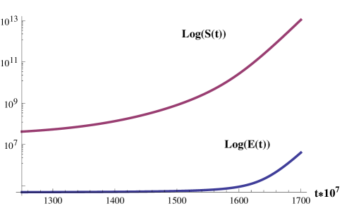
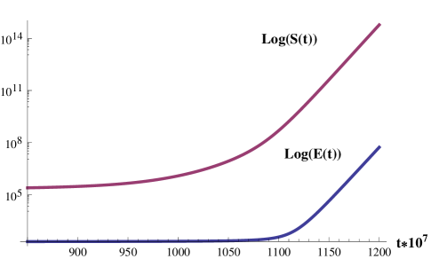
For an estimate of the critical time $\tau$ we looked first at the behavior in time of the total energy and the total enstrophy. Fig. 1 and Fig. 2 give the behavior of those quantities on a logarithmic scale, for the initial data ${\mathbf{v}}_{0}^{+}$ and ${\mathbf{v}}_{0}^{-}$, respectively. Observe that the enstrophy starts growing significantly earlier than the energy.

As we see, for the initial data ${\mathbf{v}}_{0}^{-}$ the fast growth starts earlier, at about $t\approx 10\times 10^{-5}$, than for ${\mathbf{v}}_{0}^{+}$, for which it starts at about $t\approx 15\times 10^{-5}$. Also, for ${\mathbf{v}}_{0}^{-}$ the growth is faster. This is to be expected, because, as shown in the next paragraph, for the solution with initial data ${\mathbf{v}}_{0}^{+}$ the asymptotics with alternate signs (16) holds. In what follows, we mostly report results of simulations with initial data ${\mathbf{v}}_{0}^{+}$, which are somehow easier to follow.

The growth of the total energy and total enstrophy near the critical time is predicted in [8] to be as a power law, i.e.,

$$E(t)\sim{C_{E}\over(\tau-t)^{5}},\qquad S(t)\sim{C_{S}\over(\tau-t)^{7}},$$ (20)

where $\tau$ is the critical time and $C_{E},C_{S}$ are positive constants.

It is however unclear from the analysis in [8] whether the asymptotics (20) holds with the same powers for initial data of the type ${\mathbf{v}}_{0}^{+}$, which give rise to the series with alternate signs (16). It is not easy to determine the exact powers by numerical analysis, and we need be content with compatibility estimates.

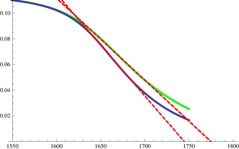
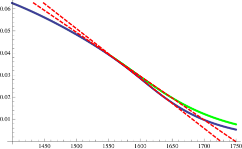
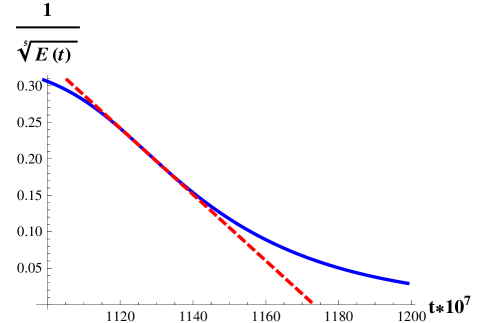
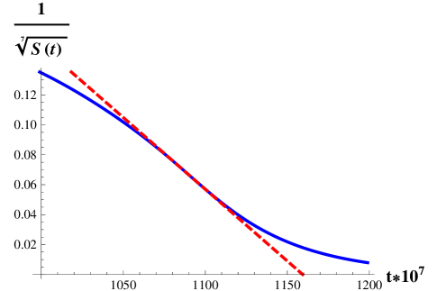
The regression plots for $(E(t))^{-{1\over 5}}$ and $(S(t))^{-{1\over 7}}$ vs $t$ are shown in Figg. 3, 4, for ${\mathbf{v}}_{0}^{+}$ and in Figg. 5,6 for ${\mathbf{v}}_{0}^{-}$. The regression is restricted to the range of times with approximately linear behavior. As we shall see in the next section, as $t$ gets close to the critical time a significant amount of “mass” gets out of the integration region, so that the growth seen in the simulations slows down. This is also the reason why, as shown in Figg. 3,4, the estimates of $\tau$, given by the intercept with the horizontal axis, decreases with $L$. As the estimates for the two values of $L$ are close to each other, for the initial data ${\mathbf{v}}_{0}^{+}$ we may take as un upper estimate for the critical time the value $\tau_{+}=1726\times 10^{-7}$.

The $R^{2}$ parameter in the linear regressions shown in Figg. 3-6 is always around $0.999$, so that we may say that the computer results are compatible with the predictions (20).

In the next paragraph we give other estimates of the critical time based on a different method.

Figure 1: Behavior of the total enstrophy $S(t)$ and the total energy $E(t)$. $L=2028$, initial data ${\mathbf{v}}_{0}^{+}$.

Figure 2: Behavior of the total enstrophy $S(t)$ and the total energy $E(t)$. $L=2028$, initial data ${\mathbf{v}}_{0}^{-}$.

Figure 3: Behavior of $(E(t))^{-{1\over 5}}$ near the blowup for $L=2028$ (green) and $L=2528$ (blue), initial data ${\mathbf{v}}_{0}^{+}$. The red dashed line is the linear regression.

Figure 4: Behavior of $(S(t))^{-{1\over 7}}$ near the blowup for $L=2028$ (green) and $L=2528$ (blue), initial data ${\mathbf{v}}_{0}^{+}$. The red dashed line is the linear regression.

Figure 5: Behavior of $(E(t))^{-{1\over 5}}$ near the blowup for $L=2528$, initial data ${\mathbf{v}}_{0}^{-}$. The red dashed line is the linear regression.

Figure 6: Behavior of $(S(t))^{-{1\over 7}}$ near the blowup for $L=2528$, initial data ${\mathbf{v}}_{0}^{-}$. The red dashed line is the linear regression.

4 Behavior of the solution in ${\mathbf{k}}$-space.

Figg. 7,8,9 show the behavior in ${\mathbf{k}}$-space of the solutions with initial data ${\mathbf{v}}_{0}^{+}$ and ${\mathbf{v}}_{0}^{-}$.

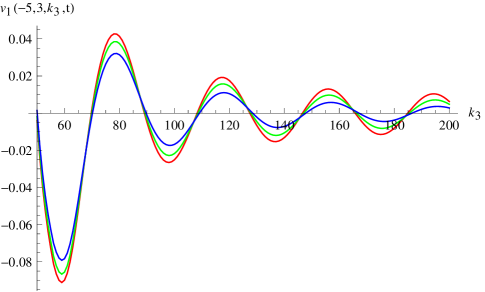
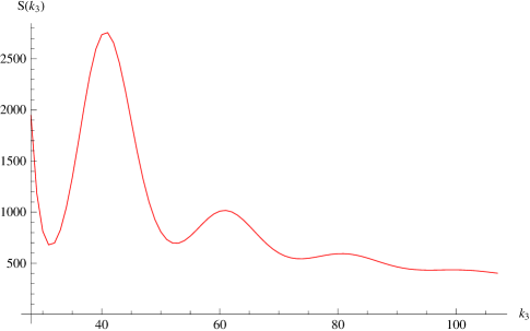
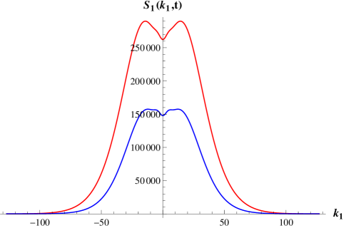
In Fig. 7 we report the plot of a transversal component of the solution with initial data ${\mathbf{v}}_{0}^{+}$, vs $k_{3}$, for $k_{1},k_{2}$ and $t$ fixed, for three values of $t$. It can be seen that the behavior of the solution is close to a damped oscillation with period $2a$, and zeroes at the points $k_{3}\approx{1\over 2}(2j+1)\;a$, $j=1,\ldots$. This is due to the alternating signs of the series (16). Moreover the data are compatible with a pointwise convergence in ${\mathbf{k}}$ to a limiting function as $t\uparrow\tau$, a fact that is presumably not hard to prove rigorously.

A look at Fig. 8, which gives, for the same initial data, the behavior of the marginal density $S_{3}(k_{3},t)$ at $t$ fixed, confirms that the solution has a sequence of zeroes with approximate distance $a$. On the other hand, for the solution coming out of ${\mathbf{v}}_{0}^{-}$, as the coefficients multiplying $\mathbf{H}^{{(0)}}({{\mathbf{k}}-{\mathbf{k}}^{{(0)}}\over\sqrt{p}})$ in the series (14) are all positive, there are no zeroes and the oscillations are visible only for small $k_{3}$ (Fig. 9).

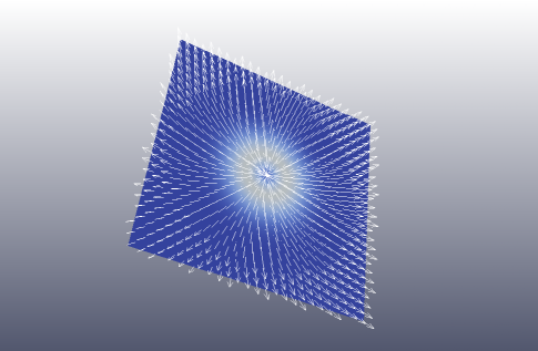
Fig. 10 shows the vectors ${\mathbf{v}}({\mathbf{k}},t)$ on the plane $k_{3}=100$ at the time $t=1521\times 10^{-7}$ for initial data ${\mathbf{v}}_{0}^{+}$. The picture is limited to the part of the plane were ${\mathbf{v}}$ is significantly nonzero. The fact that the velocity field is overwhelmingly radial is a consequence of the fact that the solution corresponds to the fixed point $\mathbf{H}^{{(0)}}({\mathbf{Y}})=-2(Y_{1},Y_{2},0)$.

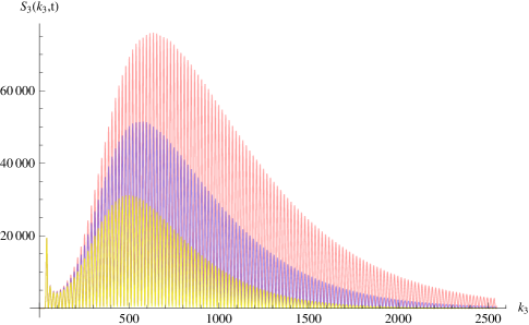
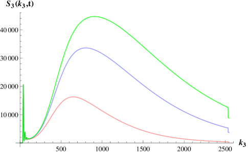
The rapid growth of the enstrophy and the time evolution of the main support of the solution along the $k_{3}$-axis are illustrated by the plot of $S_{3}(k_{3},t)$ at three different times given in Fig. 11 for ${\mathbf{v}}_{0}^{+}$ and in Fig. 12 for ${\mathbf{v}}_{0}^{-}$. As we mentioned above, for $t\uparrow\tau$ the support in ${\mathbf{k}}$-space moves away to infinity along the $k_{3}$-axis, and gets out of the integration region. Let $k^{(M)}_{3}(t)$ denote the value of $k_{3}$ where the maximum of the enstrophy marginal $S_{3}(k_{3},t)$ is located. One can predict, on the basis of the asymptotics (14), (16), that, as $t\uparrow\tau$, we should have $k^{(M)}_{3}(t)\sim{C\over\tau-t}$, for some constant $C>0$. This is shown by Fig. 13, which gives the behavior of $\log[k^{(M)}_{3}(t)(\tau-t)]$ vs $t$ for the initial data ${\mathbf{v}}^{+}$, anf for $\tau=1640\times 10^{-7}$. For this choice of the critical time, see the discussion below in this paragraph.

Concerning the transversal distribution of the enstrophy, Fig. 14 shows the plot of $S_{1}(k_{1},t)$ for the first two times as in Fig. 11. The transverse marginal $S_{2}(k_{2},t)$ looks exactly the same. As we see, the support of the solution in the transversal directions grows very slowly and is well contained inside the square $[-127,127]$ of the computation region.

For the initial data ${\mathbf{v}}_{0}^{+}$ we will use another way of predicting the explosion time, based on the decay rate of the maxima of the oscillations (bumps) in the plot of $E(k_{3},t)$, which shows the same kind of oscillations as $S(k_{3},t)$ in Fig.11. As $\Lambda(t)$ is a smooth function, the expansion (15) shows that, as $t\uparrow\tau$, for $k_{3}>k^{(M)}_{3}(t)$ the maxima, for $k_{3}$ large enough, should decay exponentially, with an exponent proportional to $\tau-t$.

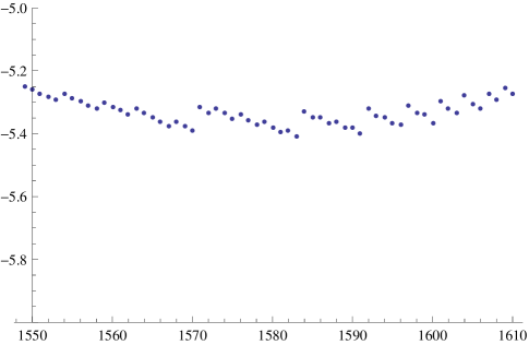
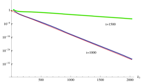
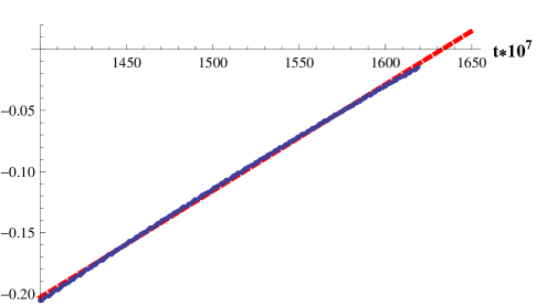
Figure 17 shows the logarithmic plot of the maxima of the peaks of $E(k_{3},t)$ versus $k_{3}$ at a fixed time $t$. The points align on straight line with great accuracy, and the slope decreases with time. Plotting the slope versus time we obtain a graph, shown on Fig. 18, which is with very good approximation a straight line (it almost coincides with its linear regression, indicated by the red dashed line). The intercept with the horizontal axis, which is around the point $t=1640\times 10^{-7}$ appears to be a lower estimate, presumably more reliable than the upper estimate, of the blow-up time $\tau$.

Figure 7: Plot of ${\mathbf{v}}_{1}({\mathbf{k}},t)$ for $k_{1},k_{2}$ fixed vs $k_{3}$, at the times $t=1342\times 10^{-7}$ (blue), $t=1500\times 10^{-7}$ (green), $t=1599\times 10^{-7}$ (red). $L=2028$, initial data ${\mathbf{v}}_{0}^{+}$.

Figure 8: Plot of $S_{3}(k_{3},t)$ vs $k_{3}$, $t=1125\times 10^{-7}$, $L=2028$, initial data ${\mathbf{v}}_{0}^{+}$.

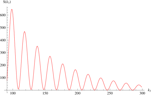
The zeroes are approximately periodic with period $a=20$.

Figure 9: Plot of $S_{3}(k_{3},t)$ vs $k_{3}$, $t=900\times 10^{-7}$. $L=2028$, initial data ${\mathbf{v}}_{0}^{-}$.

Figure 10: The vector field ${\mathbf{v}}({\mathbf{k}},t)$ on the plane $k_{3}=100$ and $t=1521\times 10^{-7}$. The arrows are assigned to a random subset of points and are proportional to the vector norm. $L=2528$, initial data ${\mathbf{v}}_{0}^{+}$.

Figure 11: $S_{3}(k_{3},t)$ at $t\cdot 10^{7}=1521,1544,1560$, $L=2528$, initial data ${\mathbf{v}}_{0}^{+}$.

Figure 12: $S_{3}(k_{3},t)$ at $t\cdot 10^{7}=1060,1075,1080$, $L=2528$, initial data ${\mathbf{v}}_{0}^{-}$.

Figure 13: Behavior of $\log[k^{M}_{3}(t)(\tau-t)]$ vs $t$, $\tau=1640\times 10^{-7}$, $L=2528$, initial data ${\mathbf{v}}_{0}^{+}$.

Figure 14: $S_{1}(k_{1},t)$ at $t\cdot 10^{7}=1521,1544$, $L=2528$, initial data ${\mathbf{v}}_{0}^{+}$.

Figure 15: Behavior of the log-plot of the maxima of the oscillations of $E_{3}(k_{3},t)$ before the blowup. $L=2028$, initial data ${\mathbf{v}}_{0}^{+}$.

Figure 16: Decay rate vs $t\times 10^{7}$ (blue), with linear regression (red). $L=2528$, initial data ${\mathbf{v}}_{0}^{+}$.

5 Behavior of the solution in $\mathbf{x}$-space

The main support in ${\mathbf{x}}$-space of the solution is always contained within a small volume around the origin, and as $t\uparrow\tau$, it concentrates in sharp “spikes” (singular points). The behavior is however qualitatively different for the initial data ${\mathbf{v}}_{0}^{+}$ and ${\mathbf{v}}_{0}^{-}$.

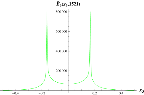
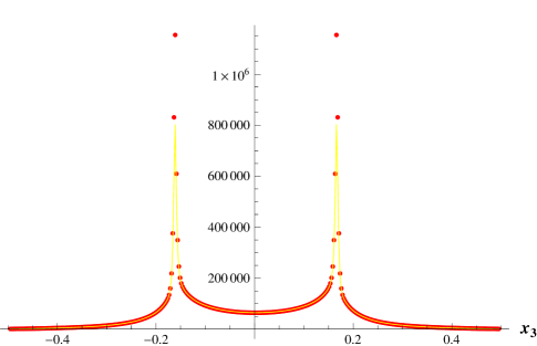
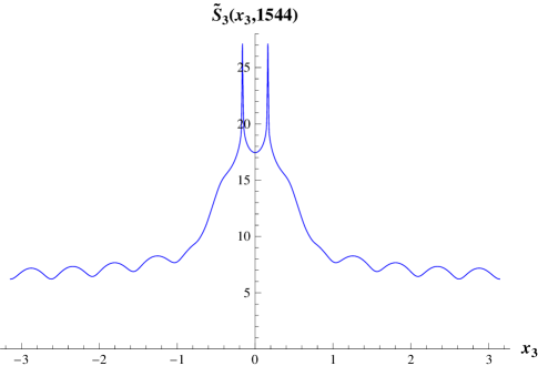
For the initial data ${\mathbf{v}}_{0}^{+}$ there are two spikes, at the points $\mathbf{x}^{{(0)}}_{\pm}=(0,0,\pm x_{3}^{{(0)}})$ with $x^{{(0)}}_{3}\approx 0.16\approx{\pi\over a}$, as one should expect in view of the fact that, as we saw, ${\mathbf{v}}({\mathbf{k}},t)$ oscilates in $k_{3}$ with a period $T\approx 2a$. Fig. 17 shows the behavior of the energy density $\tilde{E}_{3}(x_{3},t)$ for $t=1521\times 10^{-7}$.

At $x={\mathbf{x}}^{{(0)}}_{\pm}$ the energy grows to $\infty$ as $t\uparrow\tau$, as indicated by Fig. 18, which shows the growth of the maximal values of the marginal distribution $\tilde{E}_{3}(\pm x^{{(0)}}_{3},t)$. Observe that the concentration of energy begins already at $t\approx 1000\times 10^{-7}$, i.e., much earlier than the growth of the total energy.

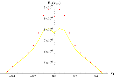
In Fig. 19 the plots of the marginal density $\tilde{E}_{3}(x_{3},t)$ at $t=1521\times 10^{-7}$ and $t=1544\times 10^{-7}$ are superimposed for comparison. Fig. 20 shows a similar comparison for the marginal density $\tilde{E}_{1}(x_{1},t)$ at the same times.

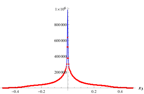
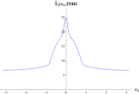
For the initial data ${\mathbf{v}}_{0}^{-}$ we have instead a single spike at the origin, as shown in Fig. 21, which shows the plots of the marginal $\tilde{E}_{3}(x_{3},t)$ at two different times.

The simulation data shown in Figg. 19, 20 and 21 suggest that the marginal densities $\tilde{E}_{1}(x_{1},t)$ and $\tilde{E}_{3}(x_{3},t)$ tend to finite limits as $t\uparrow\tau$, except at the singular points. A possible conclusion, which however would require further investigation, is that for all ${\mathbf{x}}\neq\mathbf{x}^{{(0)}}_{\pm}$ the function ${\mathbf{u}}({\mathbf{x}},t)$ itself also converges. Convergence for all points in ${\mathbf{x}}$-space except at the singular points was in fact proved for the complex Burgers equations (see [9] and [2] for computer simulations).

Except for the fact of showing a single spike, the behavior in ${\mathbf{x}}$-space of the solution for initial data ${\mathbf{v}}_{0}^{-}$ does not differ significantly, so that in what follows we will only consider the solution with initial data ${\mathbf{v}}_{0}^{+}$.

The marginal distributions of the enstrophy behave in a similar way, except that the spikes are more enhanced than for the energy marginals. Figg. 22 and Fig. 23 shows the log plot of the marginal $\tilde{S}_{3}(x_{3},t)$ and of the transverse marginal $\tilde{S}_{1}(x_{1},t)$ at a single time.

An important role with respect to possible singularities of the NS equations is played by the vorticity stretching vector $\mathbf{w}({\mathbf{x}},t)=\omega({\mathbf{x}},t)\cdot\nabla\mathbf{u}(\mathbf{x},t)$, where $\omega({\mathbf{x}},t)=\nabla\times{\mathbf{u}}({\mathbf{x}},t)$ is the vorticity (see, e.g, [11]).

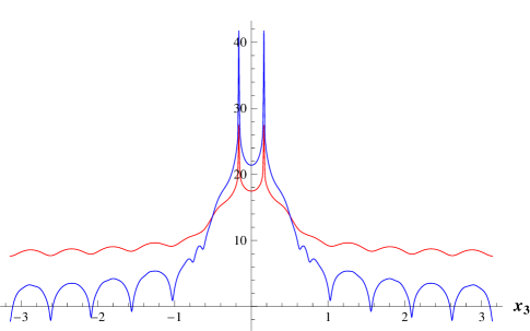
Fig. 24 shows a joint log plot nat the time $t=1544\times 10^{-7}$ of the marginals $\tilde{S}_{3}(x_{3},t)$ and

$$W_{3}(x_{3},t)=\int_{{\mathbb{R}}\times{\mathbb{R}}}dx_{1}dx_{2}\left|\omega({\mathbf{x}},t)\cdot\nabla\mathbf{u}(\mathbf{x},t)\right|^{2},$$

($W_{3}$, for dimensional homogeneity, is divided by $E_{0}$). It can be seen that $W_{3}$ is much more concentrated around the two points $\mathbf{x}^{{(0)}}_{\pm}$ than the enstrophy marginal $\tilde{S}_{3}$, which in its turn is more concentrated than the corresponding energy marginal.

Figure 17: $\tilde{E}_{3}(x_{3},t)$ at $t\cdot 10^{7}=1521$. $L=2528$, initial data ${\mathbf{v}}_{0}^{+}$.

Figure 18: Growth of $\max_{x_{3}}\tilde{E}_{3}(x_{3},t)$ in time. $L=2528$, initial data ${\mathbf{v}}_{0}^{+}$.

Figure 19: $\tilde{E}_{3}(x_{3},t)$ at $t\cdot 10^{7}=1521$ (yellow) and $t\times 10^{7}=1544$ (red dots). $L=2528$, initial data ${\mathbf{v}}_{0}^{+}$.

Figure 20: $\tilde{E}_{1}(x_{1},t)$ at $t\cdot 10^{7}=1521$ (yellow), and $t\cdot 10^{7}=1544$ (red dots). $L=2528$, initial data ${\mathbf{v}}_{0}^{+}$.

Figure 21: $\tilde{E}_{3}(x_{3},t)$ at $t\cdot 10^{7}=1021$ (red dots) and $t\times 10^{7}=1044$ (blue). $L=2528$, initial data ${\mathbf{v}}_{0}^{-}$.

Figure 22: Log-plot of $\tilde{S}_{1}(x_{1},t)$ at $t\cdot 10^{7}=1544$. $L=2528$, initial data ${\mathbf{v}}_{0}^{+}$.

Figure 23: Log-plot of $\tilde{S}_{1}(x_{1},t)$ at $t\cdot 10^{7}=1544$. $L=2528$, initial data ${\mathbf{v}}_{0}^{+}$.

Figure 24: Log-plot of $\tilde{S}_{3}(x_{3},t)$ (red) and $W_{3}(x_{3},t)$ (blue) at $t\cdot 10^{7}=1544$. $L=2528$, initial data ${\mathbf{v}}_{0}^{+}$.

6 Some data on the computer simulations

The discretization of our basic equation (5) starts with a truncation $[a_{1},b_{1}]\times[a_{2},b_{2}]\times[a_{3},b_{3}]$ of the integration region for the ${\mathbf{k}}$ variables. As we said above, all the results reported in the present paper are obtained for a uniform step size both in ${\mathbf{k}}$ and in time.

The discrete computation is obtained by the so-called Nyström method with respect to the ${\mathbf{k}}$ variables and a predictor-corrector scheme, with respect to the time variable, which is based on the Euler method and the Trapezoidal method.

The predictor-corrector scheme iterates a recursive procedure to compute successive approximations $\mathbf{V}^{(j)}({\mathbf{k}},n\delta_{t})$, $j=1,2,\ldots$, of the function ${\mathbf{v}}({\mathbf{k}},n\delta_{t})$, until a convergence criterion is satisfied: $|\mathbf{V}^{(j+1)}({\mathbf{k}},n\delta_{t})-\mathbf{V}^{(j+1)}({\mathbf{k}},n\delta_{t})|\leq{\rm tol}$, where the tolerance ${\rm tol}$ is set at $10^{-8}$.

The procedure is computationally challenging, and in fact for each ${\mathbf{k}}$ in the mesh it requires the evaluation of a three-dimensional integral. The integral is however a convolution, and by using the fast Fourier transform (FFT) we can reduce the computational cost. Note that, as we are simulating the NS equations in ${\mathbb{R}}^{3}$, the convolution is not a periodic convolution and has to be implemented on a computational grid which is doubled in size.

The accuracy of the approximated solution corresponding to the chosen initial data is evaluated on an experimental basis by comparing the results obtained for different discretization parameters.

Our computer simulations were performed at CINECA of Bologna (Italy) on the FERMI Supercomputer (Model: IBM-BlueGene/Q; Architecture: $10$ BGQ Frame; Processor Type: IBM PowerA2, $1.6$ GHz; Computing Cores $163840$; Computing Nodes $10240$; RAM: 1GByt/core)

The computation method was implemented in Fortran 90 (IBM Fortran compiler) with MPI library for parallel computations, and 2Decomp&FFT for the parallel computation of the fast Fourier transform.

7 Concluding Remarks

Simulations of the solutions of the 3-d NS equations are usually computationally onerous and sometimes unreliable, especially for flows with large values of the enstrophy and of the vorticity stretching. It is a remarkable fact that the singular complex solutions proposed by Li and Sinai in [8], due to their simple structure in ${\mathbf{k}}$-space, are relatively easy to follow by computer simulations on the supercomputers of the last generation.

Of particular importance in this respect is the representation of the solution as a power series (6), where the parameter $A$ governs the blow-up time. A great help also comes from the stability of the computation with respect to the discretization step in ${\mathbf{k}}$-space, which is due to the confinement of the energy in a small region of ${\mathbf{x}}$-space, as we discussu below. It is perhaps worth to observe that in the paper of Li and Sinai [8] the infinite extension of the domain in ${\mathbf{x}}$-space does not seem to be essential, except for the fact that there are no boundary conditions, and that the proofs can be adapted, by some straightforward modifications, to the periodic case on the torus $T^{3}$ as well.

The results of our computer simulations give a clear evidence of the blow-up, with an estimate the critical time. It was also possible to obtain a detailed picture of the behavior of the solutions near the critical time, confirming the predictions of the theory, and also producing evidence of important properties, such as the pointwise convergence as $t\uparrow\tau$ of the solution in ${\mathbf{k}}$-space, and in ${\mathbf{x}}$-space except for the singular points. Whether such properties really hold requires further study.

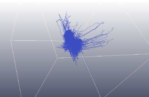
The general picture that comes out is that of a motion in which the fluid points move very fast in a small region around the origin, for the initial data ${\mathbf{v}}_{0}^{-}$, or around two symmetric points close to the origin, for the initial data ${\mathbf{v}}_{0}^{+}$, along flow lines with high curvature. Fig. 25 shows the flow lines (for the real part of ${\mathbf{u}}({\mathbf{x}},t)$) starting at $t=0$ from a random set of fluid points in a small central region and up to time 1521. One can see that the overwhelming majority of the lines is confined to the central region.

As we go to the critical time, the enstrophy, and even more the vorticity stretching, are increasingly in spikes, which diverge to infinity at the singular points, while the fluid at a finite distance remains “quiet.” A behavior which reminds that of a physical tornado.

The results so far obtained suggest the study of real-valued solutions of the 3-d NS equations which share some basic properties, such as the extension of the essential support of the solutions in ${\mathbf{k}}$-space, with the complex solutions considered in the present paper. More work in this direction is in progress.

Figure 25: Flow lines from a random set of points up to time $1541\times 10^{-7}$. $L=2528$, initial data ${\mathbf{v}}_{0}^{+}$.

8 Acknowledgements

We thank Prof. Ya. G. Sinai for his constant interest on our work, and for many discussions and suggestions. We also thank Dr D. Li for valuable remarks. We acknowledge the CINECA award under the ISCRA initiative IsB10_3DNS (2014) and IsC23_3DNS (2015), for the availability of high performance computing resources and support.

References

- [1] Arnol’d, M.D. and Khokhlov, A.V.: “Modeling a blow-up solution of tornado type for the complex version of the three dimensional Navier-Stokes equation”. Russian Mathematical Surveys, 64, 1133–1135, 2009
- [2] Boldrighini, C., Frigio, S. and Maponi, P.: “Exploding solutions of the two-dimensional Burgers equations: Computer simulations”. J. Math. Phys. 53,083101, 2012
- [3] Cheskidov, A.: “Blow-up in finite time for the dyadic model of the Navier-Stokes equations”. Trans. Am. Math. Soc., 10, 5101-5120, 2008
- [4] Hou, Th. Y.: “Blow-up or no blow-up? A unified computational and analytic approach to three-dimensional incompressible Euler and Navier-Stokes equations”. Acta Numerica, 18, 277-346, 2008
- [5] Katz, N. Pavlovic, N.: “A cheap Caffarelli-Kohn-Nirenberg inequality for the Navier-Stokes equation with hyper-dissipation”. Geom. Funct. Anal. 12, No. 2, 355-379, 2002
- [6] Leray, J.: “Sur le mouvement d’un liquide visqueux emplissant l’éspace”. Acta Math 63, 193–248, 1934
- [7] Temam, R.: Navier-Stokes Equations. North Holland, 1979
- [8] Li, D. and Sinai, Ya. G.: “Blowups of complex solutions of the 3D Navier-Stokes system and renormalization group method”. J. Eur. Math. Soc. 10, 267–313, 2008
- [9] Li, D, and Sinai, Ya.G.: “Singularities of complex-valued solutions of the two-dimensional Burgers system”. J. Math. Phys. 51, 01525, 2010
- [10] Li, D, and Sinai, Ya.G.: “Blowups of Complex-valued Solutions for Some Hydrodynamic models”. Regular and Chaotic Dynamics 15, Nos 4-5, 521-531, 2010
- [11] Ruzmaikina, A, and Grujic, Z.: “On Depletion of the Vortex-Stretching Term in the 3D Navier-Stokes Equations”. Comm. Math. Phys, 247 , 601-611, 2004
- [12] Seregin, G.: “A Certain Necessary Condition of Potential Blow up for Navier-Stokes Equations”. Commun. Math. Phys. 312, 833-845, 2012
- [13] Tao, T.: “Finite time blowup for an averaged three-dimensional Navier-Stokes equation”. arXiv: 1402.0290v2 [math AP], 2014