Wave Patterns in A Nonclassic Nonlinearly-Elastic Bar Under Riemann Data

Abstract

Recently there has been interest in studying a new class of elastic materials, which is described by implicit constitutive relations. Under some basic assumption for elasticity constants, the system of governing equations of motion for this elastic material is strictly hyperbolic but without the convexity property. In this paper, all wave patterns for the nonclassic nonlinearly elastic materials under Riemann data are established completely by separating the phase plane into twelve disjoint regions and by using a nonnegative dissipation rate assumption and the maximally dissipative kinetics at any stress discontinuity. Depending on the initial data, a variety of wave patterns can arise, and in particular there exist composite waves composed of a rarefaction wave and a shock wave. The solutions for a physically realizable case are presented in detail, which may be used to test whether the material belongs to the class of classical elastic bodies or the one wherein the stretch is expressed as a function of the stress.

Key words and phrases: implicit constitutive relation, Riemann problem, kinetic relations, wave patterns

2010 Mathematics Subject Classification: 35L65, 35L45, 74B20

1 Introduction

Until recently, models used to describe the elastic response of bodies belonged to either the class of Cauchy elastic bodies or Green elastic bodies. Recently, Rajagopal [23, 24] introduced a much larger class of elastic bodies that included Cauchy elastic bodies and Green elastic bodies as a subset, if by elastic response one refers to a response wherein the body is incapable of dissipating energy, that is, inability to convert working into thermal energy. Of particular reference to the current work are bodies defined by implicit constitutive relations between the stress and the deformation gradient, or the sub-class wherein the strain in the body is a function of the stress. Such models are relevant when one has a material wherein the body exhibits a limiting strain or when the response between the strain and stress becomes non-linear even for very small strains wherein the classical models of elasticity reduce to the classical linearized elastic model. When the elastic body exhibits limiting strain then one could encounter the possibility that the stress cannot be expressed as a function of the strain (see Rajagopal [23]). A detailed mathematical treatment of such a response can be found in Bulicek et al. [4]. With regard to the possibility of a non-linear relationship between the strain and the stress, even when the strains are very small, one needs but look at the response of alloys such as Gum metal (see Saito et al. [28]) and many other Titanium Nickel based alloys (see Talling et al. [31], Withey [35], Zhang [36]). The response of such alloys cannot be described by the classical linearized elastic response but can be described very well with the help of the new class of elastic models wherein the linearized strain is a non-linear function of the stress (see Rajagopal [26]). Another very important class of problems where the new class of models might prove to be very useful is in predicting the state of strain in the neighborhood of cracks and the tips of notches, etc. While the linearized theory of elasticity predicts strains that blow up in the neighborhood of the tip of a crack, contradicting the very precepts under which the approximation is derived, the new class predicts results that are physically meaningful in that the strains are bounded and never exceed the limit of small strain that is supposed (see Rajagopal and Walton [27], Kulvait, et al. [14]).

Nonlinear waves in elastic bars, within the traditional framework that the stress is a function of the strain, have been studied in various contexts. For example, recently Huang, Dai, Chen and Kong [11] showed that for certain nonlinearly elastic materials, it is possible to generate a phenomenon in which a tensile wave can catch the first transmitted compressive wave (so the former can be undermined) in an initially stress-free two-material bar. Depending on the interval of the initial impact, the wave catching-up phenomena can happen in two wave patterns. Some asymptotic solutions were also constructed. As a continuation of this work, Huang, Dai and Kong [10] investigated the wave catching-up phenomenon in a nonlinearly elastic prestressed two-material bar and the global structure stability of nonlinear waves was also proved by the method of characteristics and the theory of typical boundary problems. An interesting study on impact-induced phase transformation in a shape memory alloy rod was carried out by Chen and Lagoudas [6], and notably they also found that composite waves with a rarefaction wave and a shock wave can arise.

In this paper, we study the Riemann problem for a specific sub-class of the new class of elastic bodies proposed by Rajagopal and focus on the various wave patterns. These equations do not possess convexity though they are strictly hyperbolic. In this study, the Reimann problem for this special sub-class is solved completely. We find that, depending on the initial condition, a variety of wave patterns can arise including a composite wave comprising of a rarefaction wave and a shock wave. We also note that due to the implicit constitutive relation (5), it is natural to select the velocity and the stress as the unknowns. Within such a framework, the equations of motion governing the sub-class of bodies under consideration cannot be written in terms of the type of conservation laws that hold for the classical elastic body.

To introduce the kind of constitutive relation adopted in this paper, we first recall some basic definitions in kinematics. The reference configuration, denoted by $\mathcal{B}$, is assumed to be stress-free. A particle ${\bf X}\in\mathcal{B}$ occupies the position ${\bf x}\in\mathcal{B}_{t}$, where $\mathcal{B}_{t}$ is the configuration at time $t$, that is referred to as the current configuration. The mapping that maps the reference configuration to the current configuration is assumed to be one to one, and is given by ${\bf x}={\bf\chi}({\bf X},t)$. We denote the displacement by ${\bf u}={\bf x}-{\bf X}$. Then the gradients of displacement are given as

$$\frac{\partial{\bf u}}{\partial{\bf X}}=\nabla_{\bf X}{\bf u}={\bf F}-{\bf I}\quad\text{or}\quad\frac{\partial{\bf u}}{\partial{\bf x}}=\nabla_{\bf x}{\bf u}={\bf I}-{\bf F}^{-1},$$

where ${\bf F}=\frac{\partial{\bf x}}{\partial{\bf X}}$ is the deformation gradient tensor, and ${\bf I}$ is the identity tensor. The Green-Saint Venant strain ${\bf E}$ is given by

$${\bf E}=\frac{1}{2}\left(\nabla_{\bf X}{\bf u}+(\nabla_{\bf X}{\bf u})^{T}+(\nabla_{\bf X}{\bf u})^{T}\nabla_{\bf X}{\bf u}\right).$$ (1)

When one assumes that the displacement gradient is small so that the last term that appears in the right hand side of (1) can be ignored in comparison to the other terms, one obtains the linearized measure of strain. The constitutive relation for elastic response within the classical theory of Cauchy or Green elasticity then leads to the popular approximation of linearized elasticity. Recently, Rajagopal [23] (see also Rajagopal [24], [25], [26]) introduced the following implicit constitutive relation for isotropic elastic materials

$${\bf f}({\bf T},{\bf B})={\bf 0},$$ (2)

where ${\bf B}={\bf F}{\bf F^{T}}$ is the left Cauchy-Green strain tensor and ${\bf T}$ is the Cauchy stress tensor. The general class (2) includes Cauchy elastic bodies as a special sub-class and another special subclass that is useful and is given by

$${\bf B}=\tilde{\alpha}_{0}{\bf I}+\tilde{\alpha}_{1}{\bf T}+\tilde{\alpha}_{2}{\bf T}^{2},$$ (3)

where the materials moduli $\tilde{\alpha}_{i}(i=1,2,3)$ depend on the density and the principal invariants of the Cauchy stress. Under the small strain assumption

$$\max_{{\bf X}\in\mathcal{B},t\in\mathbb{R}}||\nabla_{\bf X}{\bf u}||=O(\delta),\quad\delta\ll 1,$$

where $||\cdot||$ denotes the trace norm, Rajagopal [23] obtained the approximation with $O(\delta)$ from (3) as follows

$${\bf\epsilon}=\alpha_{0}{\bf I}+\alpha_{1}{\bf T}+\alpha_{2}{\bf T}^{2},$$

where as usual the materials moduli $\alpha_{i}(i=1,2,3)$ depend on the density in current configuration and the principal invariants of Cauchy stress, $\epsilon$ is the linearized strain tensor. In particular, Kannan, Rajagopal and Saccomandi [12] proposed the following special constitutive relation:

$${\bf\epsilon}=\beta(\text{tr}{\bf T}){\bf I}+\alpha\left(1+\frac{\gamma}{2}\text{tr}{\bf T^{2}}\right)^{n}{\bf T},$$ (4)

where $\alpha\geq 0,\beta\leq 0,\gamma\geq 0$ and $n$ are constants.

There have been many studies carried out within the context of the new class of elastic bodies defined by (4). Of relevance to the current study is the paper by Kannan, Rajagopal and Saccomandi [12], wherein they investigated the unsteady motions of this new class of elastic solids. It was shown that the stress wave changes its shape since the wave speed depends on the stress and the value of stress varies according to the thickness of the slab. All these phenomena for the generated stress wave are quite different from what one observes for a classical linear elastic material.

When we restrict the constitutive relation (4) to one dimension, we obtain the one-dimensional constitutive relation

$$\epsilon=\beta T+\alpha\left(1+\frac{\gamma}{2}T^{2}\right)^{n}T.$$ (5)

We will assume that the constants in (5) satisfy that

$$\alpha>0,\quad\beta<0,\quad\gamma>0,\quad n>0.$$ (6)

Moreover, we suppose that

$$\alpha+\beta>0.$$ (7)

Remark 1.1.

The assumption (7) guarantees the following governing system of equations (8) is hyperbolic.

In this paper, we consider the Riemann problem for nonlinear wave equations

$$\rho\frac{\partial v}{\partial t}=\frac{\partial T}{\partial x},\quad\frac{\partial\epsilon}{\partial t}=\frac{\partial v}{\partial x}$$ (8)

with the initial data

$$(T,v)(0,x)=\left\{\begin{array}[]{ll}(T_{l},v_{l}),&x<0,\vspace{2mm}\\ (T_{r},v_{r}),&x>0,\end{array}\right.$$ (9)

where $t,x$ represent the time and spatial coordinate respectively, $\rho$ the density of elastic body, $T$ the Cauchy stress, $\epsilon$ the strain, $v$ the particle velocity. The constant Riemann data in (9) satisfy that $(T_{l},v_{l})\neq(T_{r},v_{r}).$

Riemann problem for PDEs is of significance not only in physics, but also in mathematics. It is well-known that the Riemann problem can be used as a building block to prove existence results for the Cauchy problem for (8) with general initial data [9], possibly having large total variation [3].

For the gas dynamics equations with convex condition, the Riemann problem has been well-studied (see [5], [29]). Wendroff [33, 34] investigated the gas dynamics equations without convexity conditions for the pressure and constructed a solution to the Riemann problem. Liu [18, 19] considered the Riemann problem for general systems of conservation laws. By introducing an extended entropy condition, which is equivalent to the Lax’s shock inequalities [15] when the system is genuinely nonlinear, Liu [19] proved the uniqueness theorem for the Riemann problem of the gas dynamics equations without convexity conditions for the pressure. By a special vanishing viscosity method, Dafermos [7] obtained the structure of solutions of the Riemann problem for a general $2\times 2$ conservation laws. Matsumura and Mei [21] considered the nonlinear asymptotic stability of viscous shock profile for a one-dimensional system of viscoelasticity, where the constitutive relation is non-convex. They applied the degenerate shock condition proposed by Nishihara [22] to single out an admissible shock solution. By introducing a generalized shock in [22], Sun and Sheng [30] constructed the solutions to the Riemann problem for a system of nonlinear degenerate wave equations in elasticity, for which the strain-stress function is nonconvex. For the same equations, by using the Liu-entropy condition in [19] alternatively, Liu and Wang [20] completely obtained the corresponding Riemann solutions, some of which are different from those in [30].

By Liu-entropy condition, LeFloch and Thanh [16] uniquely solved the Riemann problem for a nonlinear hyperbolic system describing phase transitions in elastodynamics. But it is noted that the elastic model in [16] is different from the present material by comparing the assumptions (1.3) in [16] and (5). A more related work was done by Tzavaras [32], who studied the Riemann problem for the equations of one-dimensional isothermal elastic materials by taking viscosity to be zero in the equations of viscoelasticity. Wendroff criterion was applied at shocks to select a physically admissible one. For more recent results on Riemann problems, one may refer to Chapter IX and references therein by Dafermos [8] or a monograph by LeFloch [17].

We note that while there are a number of analytical solutions available for classical elastic materials, there are few ones for the previously mentioned nonclassical materials. Considering the importance of analytical solutions and the Riemann problem, we shall solve (8) and (9) with the implicit constitutive relation analytically. The Riemann problem (8)-(9) is different from the classical one since the linearized strain is a function of stress and this function is nonconvex (cf. Remark 2.3). From the application point of view, the mathematical results on Riemann problem may be used to test whether the material belongs to the class of classical elastic bodies or the ones with an implicit constitutive relation by comparing the wave patterns in a designed experiment. Remarkably, we find that there are twelve wave patterns for the considered material, while there is only one wave pattern for a classical one with the small strain. We remark that the well-posedness for the Cauchy problem for one-dimensional strictly hyperbolic equations with small initial data has been established by Bianchini and Bressan [3]. Error estimates for the Glimm approximate solution and the vanishing viscosity solution were derived in [2].

The remaining organization of this paper is as follows: In Section 2, we briefly recall some admissibility criteria for weak solutions of hyperbolic equations. Section 3 is devoted to constructing the elementary waves for our system (8) and in Section 4, we provide all the solutions to the Riemann problem (8)-(9) case by case. Section 5 is devoted to studying the Riemann solution in detail for a physically realizable situation $v_{l}=v_{r}=0$.

2 Admissibility criteria

In the community of hyperbolic equations, one often uses the Lax entropy inequality [15] to single out the unique weak solution for genuinely nonlinear hyperbolic equations; while for general hyperbolic equations without convexity, the Liu-entropy condition ([18],[19]) is a preferable candidate, which can be viewed as a generalization of Oleinik entropy condition [8] for scalar hyperbolic conservation laws. The Liu-entropy condition reads

$$s(U_{l},U_{r})\leq s(U_{l},U)\;\text{for every}\;U\;\text{between}\;U_{l}\;\text{and}\;U_{r},$$ (10)

where $s(U_{l},U_{r})$ is the speed of a shock connecting the left state $U_{l}$ and the right state $U_{r}$. Both Lax entropy inequality and Liu-entropy condition have been justified by the method of vanishing viscosity (see Chapter VIII in Dafermos [8]). It is also worthy to point out that these two criteria can guarantee the shock waves are stable [8].

In the mechanics community, often a more physical selection criterion is used. Knowles [13] investigated the impact-induced tensile waves in a semi-infinite bar made of a rubberlike material. The governing system of equations is strictly hyperbolic, but genuine nonlinearity fails. He succeeded in constructing the corresponding solutions according to three regimes of response, depending on the intensity of the loading. For the intermediate case, there is a one-parameter family of solutions to the initial-boundary problem. In order to select the unique admissible solution, Knowles [13] introduced the concept of driving force defined via the dissipation rate (see also related discussions in the monograph by Abeyaratne and Knowles [1]) and the kinetic relations. By Eqs. (8) and the Rankine-Hugoniot conditions, the dissipation rate with shock waves can be written as (cf. [1], [13])

$$D(t)=f(t)\,s,$$ (11)

where $f(t)$ is the driving force per unit cross-sectional area acting at time $t$ and can be computed in terms of the stresses on either side of the jump by

$$f(t)=\int_{T_{r}}^{T_{l}}\varepsilon(y)dy+\frac{\varepsilon(T_{r})+\varepsilon(T_{l})}{2}(T_{r}-T_{l}),$$ (12)

$s=s(t)$ is the speed of a stress discontinuity. For the present model (5), we have

$$f(t)=\frac{\alpha}{(n+1)\gamma}[F(T_{l},T_{r})-F(T_{r},T_{l})],$$ (13)

where $F(x,y)=(1+\frac{\gamma}{2}x^{2})^{n}(1-\frac{n}{2}\gamma x^{2}+\frac{n+1}{2}\gamma xy).$ By detailed but straightforward analysis, the driving force $f(t)$ can be depicted as in Fig. 1.

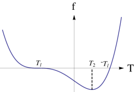
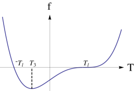
Fig. 1: Plots for $f(t)$: $T_{l}<0$ (left), $T_{l}>0$(middle) and $T_{l}=0$ (right), where $T_{2},T_{3}$ are defined through (17).

The second law of thermodynamics requires $D(t)\geq 0$. As in Knowles [13], a solution to the Riemann problem (8), (9) is called physically admissible if

$$D(t)=f(t)\,s\geq 0\;\;\text{for}\;\;t>0,$$ (14)

equivalently,

$$s\,(T_{r}-T_{l})(T_{r}+T_{l})\geq 0\;\;\text{for}\;\;t>0,$$ (15)

at every stress discontinuity. In order to obtained the uniqueness of the solution to the corresponding initial boundary value problem, Knowles [13] considered a special kinetic relation: maximally dissipative kinetics, which requires that

$$\text{either}\;\;\frac{\sigma(\gamma^{+})-\sigma(\gamma^{-})}{\gamma^{+}-\gamma^{-}}=\sigma^{\prime}(\gamma^{+})\;\;\text{or}\;\;\frac{\sigma(\gamma^{+})-\sigma(\gamma^{-})}{\gamma^{+}-\gamma^{-}}=\sigma^{\prime}(\gamma^{-})$$ (16)

must hold, where $\sigma=\sigma(\gamma)$ is the stress-response function, $\gamma^{\pm}$ are the strains on either side of a discontinuity.

In the next section, we shall discuss all backward and forward wave curves according to the cases: $T_{l}<0$, $T_{l}>0$ and $T_{l}=0$. For the case $T_{l}<0$, by the criterion (15) it is possible to construct a backward shock wave for all $T_{r}\in(T_{l},-T_{l}]$ (cf. Fig.1), while for $T_{r}>-T_{l}$, a single backward shock is thermodynamically impossible since (15) cannot be satisfied. Instead, there should appear an additional backward rarefaction wave. That is to say, when $T_{r}>-T_{l}$, we have to establish a two-wave solution composed of a rarefaction wave followed by a shock wave. However, this kind of solution is not unique since the $T$ in the middle state can lie arbitrarily in $(T_{l},-T_{l}]$. With aiming to overcome this difficulty, we apply the maximally dissipative kinetics in [13] at this solution, which requires that the $T$ in the middle state should equal $T_{2}$ given by

$$\frac{\epsilon(T_{2})-\epsilon(T_{l})}{T_{2}-T_{l}}=\epsilon^{\prime}(T_{2})\;\;\text{for}\;\;T_{l}<0\;\;\text{and}\;\;\frac{\epsilon(T_{3})-\epsilon(T_{l})}{T_{3}-T_{l}}=\epsilon^{\prime}(T_{3})\;\;\text{for}\;\;T_{l}>0,$$ (17)

where $T_{2}$ and $T_{3}$ are uniquely determined due to the specific form of the strain-stress relation (5), see Fig.2.

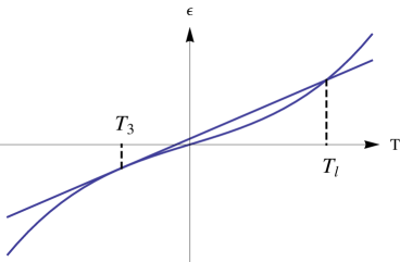
Fig. 2: The strain-stress curve and a tangent ray.

(17) is the same as (16) in terms of the inverse constitutive relation $\epsilon=\epsilon(T)$, which is the case for the nonclassic elastic material (5). Thus, by using the maximally dissipative kinetics, we arrive at a unique two-wave solution for $T_{r}>-T_{l}$. Actually, we have constructed such an elementary wave curve including two parts, one shock wave curve from $(T_{l},v_{l})$ to $(T_{2},v_{2})$ and the other rarefaction wave curve from $(T_{2},v_{2})$ to $(T_{r},v_{r})$, see Fig.4.1. If we change to use a stability criterion, such as Liu-entropy condition (10), we can construct a backward shock wave only for $T_{r}\in(T_{l},T_{2}]$ and beyond $T_{2}$, there appears a unique two-wave solution, which exactly coincides with the previous one. Interestingly, the shock wave for $T_{r}\in(T_{l},T_{2}]$ satisfies not only the Liu-entropy condition, but also the Lax entropy inequality. When $T_{r}<T_{l}$, one may obtain a forward shock wave according to the criterion (15). Moreover, this shock satisfies the Lax entropy inequality. The cases for $T_{l}>0$ and $T_{l}=0$ can be dealt with similarly. The above argument produces a reasonable observation that a physical discontinuity satisfied by the maximally dissipative kinetics must be stable. This kind of relationship between Lax entropy inequality, Liu-entropy condition and the maximally dissipative kinetics seems not revealed in the literature.

3 Elementary waves

By the method of wave curves, we next divide the discussions into three cases: $T_{l}<0,T_{l}>0$ and $T_{l}=0$. For first two cases, the phase plane is split into twelve disjoint regions and the corresponding Riemann solutions are derived. It is worth pointing out that there exist some composite wave solutions, which are composed of a rarefaction wave and a degenerate shock wave.

Let $U=\left(\begin{array}[]{c}T\\ v\end{array}\right)$, the system (8) can be rewritten as

$$U_{t}+A(U)U_{x}=0,$$ (18)

where

$$A(U)=\left(\begin{array}[]{cc}0&-\frac{1}{\epsilon^{\prime}(T)}\\ -\frac{1}{\rho}&0\end{array}\right).$$

Due to the assumption (7), it is easy to see that

$$\epsilon^{\prime}(T)=\beta+\alpha\left(1+\frac{\gamma}{2}T^{2}\right)^{n-1}\left(1+\frac{1+2n}{2}\gamma T^{2}\right)>0.$$ (19)

By direct computation, the eigenvalues of $A(U)$ read

$$\lambda_{1}=-\frac{1}{\sqrt{\rho\epsilon^{\prime}(T)}}<0<\lambda_{2}=\frac{1}{\sqrt{\rho\epsilon^{\prime}(T)}}.$$ (20)

The right eigenvectors corresponding to $\lambda_{i}(i=1,2)$ can be chosen as

$$r_{1}=\left(\begin{array}[]{c}-\rho\lambda_{1}\\ 1\end{array}\right),\quad r_{2}=\left(\begin{array}[]{c}-\rho\lambda_{2}\\ 1\end{array}\right),$$ (21)

respectively; while the left eigenvectors corresponding to $\lambda_{i}(i=1,2)$ can be taken as

$$l_{1}=(1,-\rho\lambda_{1}),\quad l_{2}=(1,-\rho\lambda_{2}),$$ (22)

respectively.

Summarizing the above argument leads to

Proposition 3.1.

Under the assumption (6)-(7), the system (18) is strictly hyperbolic with two distinct eigenvalues (see (20)), and the right (resp. left) eigenvectors can be chosen as (21) (resp. (22)).

Proposition 3.2.

Under the assumption (6)-(7), the characteristic fields $\lambda_{i}\,(i=1,2)$ for (18) are not genuinely nonlinear in the sense of Lax [15].

Proof.

It suffices to calculate the invariants $\nabla\lambda_{i}\cdot r_{i}\,(i=1,2)$. By computation,

$$\nabla\lambda_{i}\cdot r_{i}=\left(\frac{\partial\lambda_{i}}{\partial T},\frac{\partial\lambda_{i}}{\partial v}\right)\cdot\left(-\rho\lambda_{i},1\right)=-\rho\lambda_{i}\frac{\partial\lambda_{i}}{\partial T}=\frac{\epsilon^{\prime\prime}(T)}{2\left[\epsilon^{\prime}(T)\right]^{2}},$$

where

$$\epsilon^{\prime\prime}(T)=\alpha n\gamma T\left(3+\frac{1+2n}{2}\gamma T^{2}\right)\left(1+\frac{\gamma}{2}T^{2}\right)^{n-2}.$$ (23)

So the system (18) is genuinely nonlinear in the sense of Lax if $T\neq 0$, however the genuinely nonlinearity is not valid when $T=0$. Thus, the proof is completed. ∎

Remark 3.1.

By (19) and (23), the strain-stress relation $\epsilon=\epsilon(T)$ is always increasing and has concave part and convex part on $(-\infty,0]$ and $(0,+\infty)$, respectively.

Since the Riemann problem (8) and (9) are invariant under stretching of coordinates: $(t,x)\rightarrow(ct,cx)\;(c$ is a constant), we seek the self-similar solution $(T,v)(t,x)=(T,v)(\xi),\xi=x/t$. Then the Riemann problem (8)-(9) can be reduced into the following boundary value problem

$$\left\{\begin{array}[]{lll}\rho\xi v_{\xi}+T_{\xi}=0,\\ v_{\xi}+\xi\epsilon^{\prime}(T)T_{\xi}=0,\\ (T,v)(+\infty)=(T_{r},v_{r}),\\ (T,v)(-\infty)=(T_{l},v_{l}).\end{array}\right.$$ (24)

We know (24) provides either the constant state solution $U=$Const, or the singular solution, i.e., the backward (or 1-)rarefaction wave and the forward (or 2-)rarefaction wave corresponding to the eigenvalues $\lambda_{1}$ and $\lambda_{2}$, respectively.

Moreover, the system (8) admits discontinuous shock solutions, which satisfy the Rankine-Hugoniot conditions at the moving stress discontinuity located at $x=x(t)$

$$s\rho[v]+[T]=0,\quad s[\epsilon]+[v]=0,$$

where $[f]=f(t,x(t)+0)-f(t,x(t)-0)$ and $s=dx(t)/dt$ is the speed of a shock wave. If we have $s=\lambda_{i}(U_{l})$ or $s=\lambda_{i}(U_{r})$, then the shock $x=x(t)$ is called a degenerate shock. If both these equalities are fulfilled, then the discontinuity $x=x(t)$ is a so-called contact discontinuity.

Under the assumption that the strain-stress relation is convex, one can completely describe the structure of shock waves and rarefaction waves for the system of classical conservation laws (cf. [29]). However, for the nonconvex case and the system considered here, the situation is much more complicated and there appear multiple waves or composite waves, see the following discussions.

Now we consider the elementary waves for the Riemann problem (8) and (9). By definition here, an elementary wave is a single shock or a rarefaction wave, or a composite wave composed of more than one single shock or rarefaction wave. A single elementary wave can be a backward rarefaction wave, or a backward shock wave (denoted by $R_{1}$, $S_{1}$, respectively), or a forward rarefaction wave, or a forward shock wave (denoted by $R_{2}$, $S_{2}$, respectively). First, we note that

$$\frac{\partial\lambda_{1}}{\partial T}=\frac{\epsilon^{\prime\prime}(T)}{2\epsilon^{\prime}(T)\sqrt{\rho\epsilon^{\prime}(T)}}\;\left\{\begin{array}[]{ll}\geq 0,\;\;T\geq 0,\\ <0,\;\;T<0,\end{array}\right.\quad\frac{\partial\lambda_{2}}{\partial T}=-\frac{\epsilon^{\prime\prime}(T)}{2\epsilon^{\prime}(T)\sqrt{\rho\epsilon^{\prime}(T)}}\;\left\{\begin{array}[]{ll}<0,\;\;T>0,\\ \geq 0,\;\;T\leq 0.\end{array}\right.$$ (25)

By the given left state $(T_{l},v_{l})$ in the Riemann data, we divide the discussions into three cases.

Case I  $T_{l}=0$.

The backward rarefaction wave is

$$R_{1}:\quad v-v_{l}=\int_{0}^{T}\sqrt{\epsilon^{\prime}(\tau)/\rho}\;d\tau,\;\;T>0\;\;\text{or}\;\;T<0,$$ (26)

where $T>0$ or $T<0$ is determined by the requirement of $\lambda_{1}(U)>\lambda_{1}(U_{l})$ for the rarefaction waves.

The forward shock wave is given by

$$S_{2}:\quad v-v_{l}=\left\{\begin{array}[]{ll}-\sqrt{T\epsilon(T)/\rho},&T>0,\\ \sqrt{T\epsilon(T)/\rho},&T<0.\end{array}\right.$$ (27)

This shock automatically satisfies (15) and $\lambda_{2}(U_{l})>s_{2}>\lambda_{2}(U_{r}),s_{2}=1/\sqrt{\rho\,\epsilon(T)/T}.$

Case II  $T_{l}<0$.

First we consider the forward elementary waves. The forward rarefaction wave $R_{2}$ can be constructed as

$$R_{2}:\quad v-v_{l}=-\int_{T_{l}}^{T}\sqrt{\epsilon^{\prime}(\tau)/\rho}\;d\tau,\quad T_{l}<T\leq 0,\;v_{1}\leq v<v_{l},$$

where $v_{1}=v_{l}-\int_{T_{l}}^{0}\sqrt{\epsilon^{\prime}(\tau)/\rho}\;d\tau$ and $T_{l}<T\leq 0$ is determined by the requirement of $\lambda_{2}(U)>\lambda_{2}(U_{l})$ for rarefaction waves. A simple calculation shows that $\frac{dv}{dT}<0,$ and $\frac{d^{2}v}{dT^{2}}\geq 0\;(T_{l}<T\leq 0),$ where the sign of equality holds if and only if $T=0$.

If $T>0$, then the forward rarefaction wave can not be continued further since $\lambda_{2}$ is monotonically decreasing for $T>0$ (see the second equation in (25)). In fact, the $R_{2}$ curve can be continued by a forward degenerate shock curve

$$S_{2}:\quad v=v_{1}-\sqrt{T\epsilon(T)/\rho}=v_{l}-\int_{T_{l}}^{0}\sqrt{\epsilon^{\prime}(\tau)/\rho}\;d\tau-\sqrt{T\epsilon(T)/\rho},\;\;T>0,$$

where this degenerate shock wave satisfies the criterion (15) and $\lambda_{2}(U_{1})=s_{2}>\lambda_{2}(U_{r}),\;U_{1}=(0,v_{1}).$

Thus, for any state $U$ with $T>0$, we can connect the left state $U_{l}$ and the right state $U$ by a forward rarefaction wave and a degenerate shock wave. This kind of wave is often called as a composite wave or a multiple wave, which changes continuously through the rarefaction wave $R_{2}$ from $(T_{l},v_{l})$ to $(0,v_{1})$ and then jumps at the right side of $R_{2}$ from $(0,v_{1})$ to $(T,v)$.

On the other hand, when $T<T_{l}$, since $\lambda_{2}$ is an increasing function (see the second equation in (25)), we can not connect the left state $U_{l}$ by a forward rarefaction wave $R_{2}$. Actually, we can construct the following shock wave

$$S_{2}:\quad v-v_{l}=\sqrt{(T-T_{l})[\epsilon(T)-\epsilon(T_{l})]/\rho},\quad T<T_{l},$$ (28)

which is the classical shock wave satisfying (15) and moreover $\lambda_{2}(U_{l})>s_{2}>\lambda_{2}(U_{r}).$

Now we consider the backward elementary waves. As discussed in Section 2, for any $T\in(T_{l},T_{2}]$, it is possible to connect the left state $U_{l}$ and a right state $U$ by a backward shock wave as follows

$$S_{1}:\quad v-v_{l}=\sqrt{(T-T_{l})[\epsilon(T)-\epsilon(T_{l})]},\quad T_{l}<T<T_{2},\;\;v_{l}<v<v_{2},$$

where $v_{2}=v_{l}+\sqrt{(T_{2}-T_{l})[\epsilon(T_{2})-\epsilon(T_{l})]}=v_{l}+(T_{2}-T_{l})\sqrt{\epsilon^{\prime}(T_{2})/\rho},$ in which we have made use of (17)₁. We find that $\lambda_{1}(U_{l})>s_{1}>\lambda_{1}(U_{r}).$ Especially, if $T=T_{2}$, then this shock wave becomes a degenerate shock since $\lambda_{1}(U_{l})>s_{1}=\lambda_{1}(U_{r}).$

Furthermore, when the stress $T>T_{2}$, as discussed previously, we have to continue the wave curve after $T=T_{2}$ by a backward rarefaction wave:

$$R_{1}:\quad v=v_{2}+\int_{T_{2}}^{T}\sqrt{\epsilon^{\prime}(\tau)/\rho}\;d\tau=v_{l}+(T_{2}-T_{l})\sqrt{\epsilon^{\prime}(T_{2})/\rho}+\int_{T_{2}}^{T}\sqrt{\epsilon^{\prime}(\tau)/\rho}\;d\tau,\;T>T_{2}.$$

Thus, for any state $U=(T,v)$ with $T>T_{2}$, we can connect the left state $U_{l}$ and the right state $U$ by a composite wave, which is composed of an $S_{1}$ wave and a $R_{1}$ wave. This composite wave jumps at the left edge of the $R_{1}$ rarefaction wave from $U_{l}$ to $(T_{2},v_{2})$ and then changes continuously through $R_{1}$ from $(T_{2},v_{2})$ to $U$.

On the other hand, for $T<T_{l}$, we can connect the left state $U_{l}$ and the right state $U$ by a backward rarefaction wave

$$R_{1}:\quad v-v_{l}=\int_{T_{l}}^{T}\sqrt{\epsilon^{\prime}(\tau)/\rho}\;d\tau,\quad T<T_{l},$$

where $T<T_{l}$ is determined by $\lambda_{1}(U)>\lambda_{1}(U_{l})$ for a rarefaction wave.

Case III  $T_{l}>0$.

We first consider the backward elementary waves. For $T>T_{l}$, we obtain the following $R_{1}$ rarefaction wave

$$R_{1}:\quad v-v_{l}=\int_{T_{l}}^{T}\sqrt{\epsilon^{\prime}(\tau)/\rho}\;d\tau,\quad T>T_{l}>0,$$

where $T>T_{l}>0$ is due to $\lambda_{1}(U)>\lambda_{1}(U_{l})$ for rarefaction waves.

As discussed in Section 2, for any $T\in[T_{3},T_{l})$, the physical admissibility (15) holds and moreover $\lambda_{1}(U_{l})>s_{1}\geq\lambda_{1}(U)$, where $U$ is the right state. So we have the backward shock wave

$$S_{1}:\quad v-v_{l}=-\sqrt{(T-T_{l})[\epsilon(T)-\epsilon(T_{l})]/\rho},\quad T_{3}\leq T<T_{l},\;v_{3}\leq v<v_{l},$$

where $v_{3}=v_{l}-\sqrt{(T_{3}-T_{l})[\epsilon(T_{3})-\epsilon(T_{l})]/\rho}$. Furthermore, if the stress $T$ is smaller than $T_{3}$, as mentioned in Section 2, the shock wave curve can not be continued and we have to continue the solution by $R_{1}$. The $R_{1}$ rarefaction wave is given by

$$R_{1}:\quad v-v_{3}=\int_{T_{3}}^{T}\sqrt{\epsilon^{\prime}(\tau)/\rho}\;d\tau,\quad T<T_{3}.$$

Now we turn to discuss the forward elementary waves. The forward shock wave $S_{2}$ is given by

$$S_{2}:\quad v-v_{l}=-\sqrt{(T-T_{l})[\epsilon(T)-\epsilon(T_{l})]/\rho},\quad T>T_{l}>0,$$ (29)

where $T>T_{l}>0$ implies the criterion (15) and $\lambda_{2}(U_{l})>s_{2}>\lambda_{2}(U)$.

For the case $0\leq T<T_{l}$, we can construct the following forward rarefaction wave

$$R_{2}:\quad v-v_{l}=-\int_{T_{l}}^{T}\sqrt{\epsilon^{\prime}(\tau)/\rho}\;d\tau,\quad 0\leq T<T_{l},v_{l}<v\leq v_{4},$$

where $v_{4}=v_{l}-\int_{T_{l}}^{0}\sqrt{\epsilon^{\prime}(\tau)/\rho}\;d\tau$ and the condition $0\leq T<T_{l}$ is derived by the requirement that $\lambda_{2}(U)>\lambda_{2}(U_{l})$ for rarefaction waves.

For $T<0$, we can not connect the left state $U_{l}$ and the right state $U$ by the above $R_{2}$ wave. We resort to a forward shock wave

$$S_{2}:\quad v=v_{1}+\sqrt{T\epsilon(T)/\rho}=v_{l}-\int_{T_{l}}^{0}\sqrt{\epsilon^{\prime}(\tau)/\rho}\;d\tau+\sqrt{T\epsilon(T)/\rho},\;T<0<T_{l},$$

where $T<0<T_{l}$ implies the physical admissibility (15) and $\lambda_{2}(U_{l})>s_{2}>\lambda_{2}(U)$.

Thus, for any state $U$ with $T<0$, we can connect the states $U_{l}$ and $U$ by a composite wave composed of a forward rarefaction wave and a forward shock wave. This wave changes continuously through the rarefaction wave $R_{2}$ from $U_{l}$ to the state $(0,v_{4})$ and then jumps at the right edge of $R_{2}$ from $(0,v_{4})$ to $U$.

4 Global solutions to the Riemann problem

In this section, we construct the global Riemann solution to (8)-(9) according to the locations of $U_{l}$ and $U_{r}$ in the $(T,v)$ plane.

First, we place all of the wave curves $R_{i}=R_{i}(T;U_{l}),S_{i}=S_{i}(T;U_{l})(i=1,2)$ in the $(T,v)$ plane and find that their distributions vary according to $T_{l}<0,T_{l}=0$ and $T_{l}>0$, see Fig. 3. Thus, in what follows, we divide the discussions for the Riemann problem (8)-(9) into three cases $T_{l}<0$, $T_{l}>0$ and $T_{l}=0$.

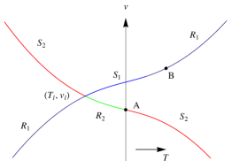
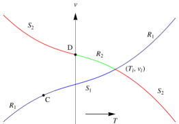
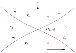
Fig. 3: Wave curves for $T_{l}<0$ (left), $T_{l}>0$ (middle) and $T_{l}=0$ (right), where the coordinates of A and B are $(0,v_{1})$ and $(T_{2},v_{2})$, respectively, in which $v_{1}=v_{l}-\int_{T_{l}}^{0}\sqrt{\epsilon^{\prime}(\tau)/\rho}\;d\tau$ and $v_{2}=v_{l}+(T_{2}-T_{l})\sqrt{\epsilon^{\prime}(T_{2})/\rho}$, and the coordinates of C and D are $(T_{3},v_{3})$ and $(0,v_{4})$, respectively, in which $v_{3}=v_{l}-\sqrt{(T_{3}-T_{l})[\epsilon(T_{3})-\epsilon(T_{l})]/\rho}$ and $v_{4}=v_{l}-\int_{T_{l}}^{0}\sqrt{\epsilon^{\prime}(\tau)/\rho}\;d\tau$.

Case A $\quad T_{l}<0$.

Referring to Fig. 3, it is well-known that the wave curves $R_{i}(T;U_{l})$ and $S_{i}(T;U_{l})$ $(i=1,2)$ have second-order contact at the point $(T_{l},v_{l})$ (cf. [29]). Moreover, we can prove that $R_{i}(T;U_{l})$ and $S_{i}(T;U_{l})\,(i=1,2)$ are twice continuously differentiable at the points A and B. As a matter of fact, in the neighborhood of point B, the shock wave and the rarefaction wave are given by

$$S_{1}(T;U_{l}):\quad v=v_{l}+\sqrt{(T-T_{l})[\epsilon(T)-\epsilon(T_{l})]/\rho},\quad T_{l}<T\leq T_{2},$$

and

$$R_{1}(T;U_{l}):\quad v=v_{l}+(T_{2}-T_{l})\sqrt{\epsilon^{\prime}(T_{2})/\rho}+\int_{T_{2}}^{T}\sqrt{\epsilon^{\prime}(\tau)/\rho}\;d\tau,\quad T>T_{2},$$

respectively, where $T_{2}$ is determined by (17). First, it is easy to see that

$$\lim_{T\rightarrow T_{2}}\frac{\partial S_{1}(T;U_{l})}{\partial T}=\lim_{T\rightarrow T_{2}}\frac{\partial R_{1}(T;U_{l})}{\partial T}=\sqrt{\frac{1}{\rho}\,\epsilon^{\prime}(T_{2})},$$

where we have made use of (17). In addition, direct computation shows

$$\frac{\partial^{2}R_{1}(T;U_{l})}{\partial T^{2}}=\frac{\epsilon^{\prime\prime}(T)}{2\sqrt{\rho\,\epsilon^{\prime}(T)}},$$

and

$$\frac{\partial^{2}S_{1}(T;U_{l})}{\partial T^{2}}=\frac{2\epsilon^{\prime}(T)+(T-T_{l})\epsilon^{\prime\prime}(T)}{2\sqrt{\rho\,(T-T_{l})[\epsilon(T)-\epsilon(T_{l})]}}-\frac{[\epsilon(T)-\epsilon(T_{l})+(T-T_{l})\epsilon^{\prime}(T)]^{2}}{4\rho^{2}[(T-T_{l})(\epsilon(T)-\epsilon(T_{l}))/\rho]^{3/2}}.$$

So by using (17), we obtain

$$\lim_{T\rightarrow T_{2}}\frac{\partial^{2}S_{1}(T;U_{l})}{\partial T^{2}}=\lim_{T\rightarrow T_{2}}\frac{\partial^{2}R_{1}(T;U_{l})}{\partial T^{2}}=\frac{\epsilon^{\prime\prime}(T_{2})}{2\sqrt{\rho\,\epsilon^{\prime}(T_{2})}}.$$

Thus, the curves $R_{1}$ and $S_{1}$ have second-order contact at the point B. It is also true for the curves $R_{2}$ and $S_{2}$ at the point A. This property for wave curves is still valid in other cases. The proof is very similar and is omitted here.

For convenience of discussion, we denote

$$\mathcal{F}(U_{l})=\left\{W_{2}(\tilde{U})\left|\tilde{U}\in W_{1}(U_{l})\right.\right\},$$

where $W_{1}(U)=R_{1}(T;U)\bigcup S_{1}(T;U)\bigcup R_{1}(T;U_{B})$ is the backward elementary wave curve issuing from $U$, in which $U_{B}$ is the state at the point B, while $W_{2}(U)$ denotes the forward elementary wave curve issuing from $U$. From Fig. 3, we know that if the stress on the left state does not vanish, then $W_{2}(U)=S_{2}(T;U)\bigcup R_{2}(T;U)\bigcup S_{2}(T;U)$; if the stress on the left state equals zero, $W_{2}(U)=S_{2}(T;U)$, see Fig. 4.

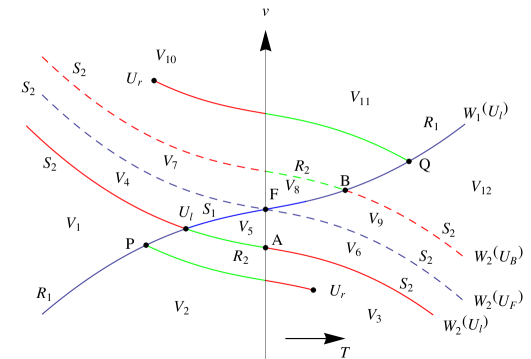
Fig. 4: Wave curves for the case $T_{l}<0$, where the coordinates of points P and Q are denoted by $(\bar{T},\bar{v})$ and $(\hat{T},\hat{v})$, respectively and the coordinates of points B and F are given by $(T_{2},v_{2})$ and $(0,v_{l}+\sqrt{T_{l}\,\epsilon(T_{l})/\rho})$, respectively.

Summarizing the preceding discussions, we have

Proposition 4.1.

The functions $W_{i}(U)\,(i=1,2)$ of the elementary wave curves are strictly monotone and twice continuously differentiable with respect to $T$.

We note that the wave curves vary dramatically according to the locations of $U_{l}$, see Fig. 3. For the present case $T_{l}<0$, by the wave curves $W_{1}(U_{l}),W_{2}(U_{l}),W_{2}(U_{B})$, $W_{2}(U_{F})$ and the line $T=0$, the phase plane $(T,v)$ is divided into twelve disjoint regions V_i $(i=1,2,\cdots,12)$, see Fig. 4.

Let $U_{l}$ be fixed and allow $U_{r}$ to vary. As discussed in Smoller [29], if $U_{r}$ lies on either $R_{i}$ or $S_{i}$ $(i=1,2)$, then the Riemann problem (8)-(9) can be solved as in the previous section. In order to obtain the general solution to the Riemann problem (8)-(9), we need to prove that the twelve disjoint regions V_i $(i=1,2,\cdots,12)$ are covered univalently by the family of curves in $\mathcal{F}(U_{l})$. That is to say, through each point $U_{r}\in$ $\bigcup_{i=1}^{12}$V_i, there passes exactly one curve in $\mathcal{F}(U_{l})$.

Suppose $U_{r}\in$ V₃. Referring to Fig. 4, we have the following equations

$$\quad\bar{v}=v_{l}+\int_{T_{l}}^{\bar{T}}\sqrt{\epsilon^{\prime}(\tau)/\rho}\;d\tau,$$ (30)

and

$$v_{r}=\left\{\begin{array}[]{lll}\bar{v}-\int_{\bar{T}}^{T}\sqrt{\epsilon^{\prime}(\tau)/\rho}\;d\tau,&\bar{T}<T\leq 0,\vspace{2mm}\\ \bar{v}-\int_{\bar{T}}^{0}\sqrt{\epsilon^{\prime}(\tau)/\rho}\;d\tau-\sqrt{T\epsilon(T)/\rho},&0<T<T_{r}.\end{array}\right.$$ (31)

In order to show the region V₃ is covered univalently by the family of curves in $\mathcal{F}(U_{l})$, it suffices to show that $\partial T/\partial\bar{v}>0$. By (30)-(31), we compute

$$1=\sqrt{\frac{\epsilon^{\prime}(\bar{T})}{\rho}}\frac{\partial\bar{T}}{\partial\bar{v}},\quad 0=\left\{\begin{array}[]{lll}1-\sqrt{\frac{\epsilon^{\prime}(T)}{\rho}}\frac{\partial T}{\partial\bar{v}}+\sqrt{\frac{\epsilon^{\prime}(\bar{T})}{\rho}}\frac{\partial\bar{T}}{\partial\bar{v}},&\bar{T}<T\leq 0,\vspace{2mm}\\ 1+\sqrt{\frac{\epsilon^{\prime}(\bar{T})}{\rho}}\,\frac{\partial\bar{T}}{\partial\bar{v}}-\frac{\epsilon(T)+T\epsilon^{\prime}(T)}{2\sqrt{\rho T\epsilon(T)}}\,\frac{\partial T}{\partial\bar{v}},&0<T<T_{r}.\end{array}\right.$$

Then, it follows that

$$\frac{\partial T}{\partial\bar{v}}=\left\{\begin{array}[]{lll}\frac{2}{\sqrt{\epsilon^{\prime}(T)/\rho}}>0,&\bar{T}<T\leq 0,\vspace{2mm}\\ \frac{4\sqrt{\rho T\epsilon^{\prime}(T)}}{\epsilon(T)+T\epsilon^{\prime}(T)}>0,&0<T<T_{r}.\end{array}\right.$$

When $U_{r}$ lies in other regions, the proof is very similar and the details are omitted.

Thus, the Riemann problem (8)-(9) can be solved by connecting $U_{l}$ and $\bar{U}$ by a backward (shock, or rarefaction, or composite) wave, and then connecting $\bar{U}$ and $U_{r}$ by a forward (shock, or rarefaction, or composite) wave.

Next, we list the Riemann solutions according to the locations of $U_{r}$ case by case.

Case A1 If $U_{r}\in$ V₁, then the Riemann solution is $U_{l}\overset{R_{1}}{\longrightarrow}\bar{U}\overset{S_{2}}{\longrightarrow}U_{r},$ where $\bar{U}=(\bar{T},\bar{v})$ is the intermediate state. The above formula means that the state $\bar{U}$ can be connected to $U_{l}$ on the right by a backward rarefaction wave and $U_{r}$ is connected to $\bar{U}$ on the right by a forward shock. The symbols below have similar meanings and we shall not explain them again unless it is necessary.

Case A2 If $U_{r}\in$ V₂, then the Riemann solution is $U_{l}\overset{R_{1}}{\longrightarrow}\bar{U}\overset{R_{2}}{\longrightarrow}U_{r}.$

Case A3 If $U_{r}\in$ V₃, then the Riemann solution is $U_{l}\overset{R_{1}}{\longrightarrow}\bar{U}\overset{R_{2}}{\longrightarrow}(0,v_{*})\xrightarrow[s_{2}=\lambda_{2}(0)]{S_{2}}U_{r},$ where $v_{*}=\bar{v}-\int_{\bar{T}}^{0}\sqrt{\epsilon^{\prime}(\tau)/\rho}\;d\tau$.

Case A4 If $U_{r}\in$ V₄, then the Riemann solution is $U_{l}\overset{S_{1}}{\longrightarrow}\bar{U}\overset{S_{2}}{\longrightarrow}U_{r}.$

Case A5 If $U_{r}\in$ V₅, then the Riemann solution is $U_{l}\overset{S_{1}}{\longrightarrow}\bar{U}\overset{R_{2}}{\longrightarrow}U_{r}.$

Case A6 If $U_{r}\in$ V₆, then the Riemann solution is $U_{l}\overset{S_{1}}{\longrightarrow}\bar{U}\overset{R_{2}}{\longrightarrow}(0,v_{*})\xrightarrow[s_{2}=\lambda_{2}(0)]{S_{2}}U_{r}.$

Case A7 If $U_{r}\in$ V₇, then the Riemann solution is $U_{l}\overset{S_{1}}{\longrightarrow}\bar{U}\overset{R_{2}}{\longrightarrow}(0,v_{*})\xrightarrow[s_{2}=\lambda_{2}(0)]{S_{2}}U_{r}.$ The structure of this solution is similar to that in Case A6.

Case A8 If $U_{r}\in$ V₈, then the Riemann solution is $U_{l}\overset{S_{1}}{\longrightarrow}\bar{U}\overset{R_{2}}{\longrightarrow}U_{r},$ which has a similar structure to that in Case A5.

Case A9 If $U_{r}\in$ V₉, then the Riemann solution is $U_{l}\overset{S_{1}}{\longrightarrow}\bar{U}\overset{S_{2}}{\longrightarrow}U_{r},$ which is similar to Case A4.

Case A10 If $U_{r}\in$ V₁₀, then the Riemann solution is

$$U_{l}\xrightarrow[s_{1}=\lambda_{1}(T_{2})]{S_{1}}U_{B}\overset{R_{1}}{\longrightarrow}\bar{U}\overset{R_{2}}{\longrightarrow}(0,v_{*})\xrightarrow[s_{2}=\lambda_{2}(0)]{S_{2}}U_{r},$$

where $U_{B}=(T_{2},v_{2})=(T_{2},v_{l}+(T_{2}-T_{l})\sqrt{\epsilon^{\prime}(T_{2})/\rho})$, in which $T_{2}$ is given by (17).

Case A11 If $U_{r}\in$ V₁₁, then the Riemann solution is $U_{l}\xrightarrow[s_{1}=\lambda_{1}(T_{2})]{S_{1}}U_{B}\overset{R_{1}}{\longrightarrow}\bar{U}\overset{R_{2}}{\longrightarrow}U_{r}.$

Case A12 If $U_{r}\in$ V₁₂, then the Riemann solution is $U_{l}\xrightarrow[s_{1}=\lambda_{1}(T_{2})]{S_{1}}U_{B}\overset{R_{1}}{\longrightarrow}\bar{U}\overset{S_{2}}{\longrightarrow}U_{r}.$

So we have solved the Riemann problem (8)-(9) for the case $T_{l}<0$.

Case B $\quad T_{l}>0$.

For this case, we are able to construct the solutions to the Riemann problem (8)-(9) by a very similar method to that in Case A. We first draw all the wave curves in the $(T,v)$ phase plane and also split the entire plane into twelve disjoint regions V${}_{i}(i=1,2,\cdots,12)$ by the wave curves $W_{1}(U_{l}),W_{2}(U_{l}),W_{2}(U_{E}),W_{2}(U_{C})$ and the line $T=0$, see Fig. 5.

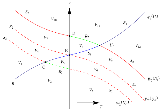
Fig. 5: Riemann solutions for the case $T_{l}>0$, where the coordinates for C, D and E are $(T_{3},v_{3}),(0,v_{4})$ and $(0,v_{l}-\sqrt{T_{l}\,\epsilon(T_{l})/\rho}\,)$, respectively.

As before, we can prove that each region V_i is covered univalently by the family of curves $\mathcal{F}(U_{l})$. So if $U_{r}$ lies in each wave curves, then the Riemann solution can be derived easily as in the previous section; while, if $U_{r}$ lies in one of regions V${}_{i}(i=1,2,\cdots,12)$, we can construct the corresponding Riemann solution as follows.

Case B1 If $U_{r}\in$ V₁, then the Riemann solution is $U_{l}\xrightarrow[s_{1}=\lambda_{1}(T_{3})]{S_{1}}U_{C}\overset{R_{1}}{\longrightarrow}\bar{U}\overset{S_{2}}{\longrightarrow}U_{r},$ where $U_{C}=(T_{3},v_{3})=(T_{3},v_{l}-\sqrt{(T_{3}-T_{l})[\epsilon(T_{3})-\epsilon(T_{l})]/\rho}\,)$, in which $T_{3}$ is determined by (17).

Case B2 If $U_{r}\in$ V₂, then the Riemann solution is $U_{l}\xrightarrow[s_{1}=\lambda_{1}(T_{3})]{S_{1}}U_{C}\overset{R_{1}}{\longrightarrow}\bar{U}\overset{R_{2}}{\longrightarrow}U_{r}.$

Case B3 If $U_{r}\in$ V₃, then the Riemann solution is $U_{l}\xrightarrow[s_{1}=\lambda_{1}(T_{3})]{S_{1}}U_{C}\overset{R_{1}}{\longrightarrow}\bar{U}\overset{R_{2}}{\longrightarrow}(0,v_{*})\xrightarrow[s_{2}=\lambda_{2}(0)]{S_{2}}U_{r},$ where $v_{*}=\bar{v}-\int_{\bar{T}}^{0}\sqrt{\epsilon^{\prime}(\tau)/\rho}\;d\tau$.

Case B4 If $U_{r}\in$ V₄, then the Riemann solution is $U_{l}\overset{S_{1}}{\longrightarrow}\bar{U}\overset{S_{2}}{\longrightarrow}U_{r}.$

Case B5 If $U_{r}\in$ V₅, then the Riemann solution is $U_{l}\overset{S_{1}}{\longrightarrow}\bar{U}\overset{R_{2}}{\longrightarrow}U_{r}.$

Case B6 If $U_{r}\in$ V₆, then the Riemann solution is $U_{l}\overset{S_{1}}{\longrightarrow}\bar{U}\overset{R_{2}}{\longrightarrow}(0,v_{*})\xrightarrow[s_{2}=\lambda_{2}(0)]{S_{2}}U_{r}.$

Case B7 If $U_{r}\in$ V₇, then the Riemann solution is $U_{l}\overset{S_{1}}{\longrightarrow}\bar{U}\overset{R_{2}}{\longrightarrow}(0,v_{*})\xrightarrow[s_{2}=\lambda_{2}(0)]{S_{2}}U_{r}.$

Case B8 If $U_{r}\in$ V₈, then the Riemann solution is $U_{l}\overset{S_{1}}{\longrightarrow}\bar{U}\overset{R_{2}}{\longrightarrow}U_{r}.$

Case B9 If $U_{r}\in$ V₉, then the Riemann solution is $U_{l}\overset{S_{1}}{\longrightarrow}\bar{U}\overset{S_{2}}{\longrightarrow}U_{r}.$

Case B10 If $U_{r}\in$ V₁₀, then the Riemann solution is $U_{l}\overset{R_{1}}{\longrightarrow}\bar{U}\overset{R_{2}}{\longrightarrow}(0,v_{*})\xrightarrow[s_{2}=\lambda_{2}(0)]{S_{2}}U_{r}.$

Case B11 If $U_{r}\in$ V₁₁, then the Riemann solution is $U_{l}\overset{R_{1}}{\longrightarrow}\bar{U}\overset{R_{2}}{\longrightarrow}U_{r}.$

Case B12 If $U_{r}\in$ V₁₂, then the Riemann solution is $U_{l}\overset{R_{1}}{\longrightarrow}\bar{U}\overset{S_{2}}{\longrightarrow}U_{r}.$

So we have finished the construction of Riemann solutions for the Case B.

Case C $\quad T_{l}=0$.

In this case, we place the wave curves $R_{1}(T;U_{l})$ and $S_{2}(T;U_{l})$ in the $(T,v)$ plane, where $R_{1}(T;U_{l})$ and $S_{2}(T;U_{l})$ are given by (26) and (27), respectively. It is seen that the $(T,v)$ plane is divided into six disjoint regions V${}_{i}\,(i=1,2,\cdots,6)$, see Fig. 3. Similarly, one can verify that each region V_i can be covered univalently by the family of curves in $\mathcal{F}(U_{l})$. So the Riemann problem (8)-(9) can be solved as in the following forms.

Case C1 If $U_{r}\in$ V₁, then the Riemann solution is $U_{l}\overset{R_{1}}{\longrightarrow}\bar{U}\overset{S_{2}}{\longrightarrow}U_{r}$.

Case C2 If $U_{r}\in$ V₂, then the Riemann solution is $U_{l}\overset{R_{1}}{\longrightarrow}\bar{U}\overset{R_{2}}{\longrightarrow}U_{r}$.

Case C3 If $U_{r}\in$ V₃, then the Riemann solution is $U_{l}\overset{R_{1}}{\longrightarrow}\bar{U}\overset{R_{2}}{\longrightarrow}(0,v_{*})\xrightarrow[s_{2}=\lambda_{2}(0)]{S_{2}}U_{r}$.

Case C4 If $U_{r}\in$ V₄, then the Riemann solution is $U_{l}\overset{R_{1}}{\longrightarrow}\bar{U}\overset{R_{2}}{\longrightarrow}(0,v_{*})\xrightarrow[s_{2}=\lambda_{2}(0)]{S_{2}}U_{r}$.

Case C5 If $U_{r}\in$ V₅, then the Riemann solution is $U_{l}\overset{R_{1}}{\longrightarrow}\bar{U}\overset{R_{2}}{\longrightarrow}U_{r}$.

Case C6 If $U_{r}\in$ V₆, then the Riemann solution is $U_{l}\overset{R_{1}}{\longrightarrow}\bar{U}\overset{S_{2}}{\longrightarrow}U_{r}$.

So we have obtained the Riemann solutions completely for the Case C.

Thus, we have obtained the globally unique piecewise smooth solutions to the Riemnn problem (8)-(9). Summarizing the above discussions, we have

Theorem 4.1.

There exists a unique piecewise smooth solution to the Riemnn problem (8)-(9) with any given initial Riemann data. These solutions are composed of constant states, backward (forward) rarefaction wave, backward (forward) shock wave and composite wave, which is a combination of rarefaction wave and shock wave.

5 A physically realizable case

In this section, we consider a case which can be realized in an experimental setting. Consider an infinitely-long circular elastic rod which is bonded by a thin rigid ring around its middle section (say, at $x=0$). Axial forces are applied to generate a stress $T_{l}$ for the part of $x<0$ and a stress $T_{r}$ for the part of $x>0$. Then, the rigid ring is released, and stress waves will be generated. Mathematically, this corresponds to the Riemann problem (8)-(9) with the velocities $v_{l}=v_{r}=0$. Although it is a special case contained in the general results given the previous section, we provide more details for the Riemann solutions due to the physical relevance.

First we make some preliminary observations. When $T_{l}<0$, by referring to Fig. 4, we denote the horizontal coordinates of the intersections for curves $W_{2}(U_{F}),W_{2}(U_{B})$ and the axes $v=0$ by $T_{*}$ and $T_{**}$, respectively. By Eq. (27) and Eq. (29) and the formulas for the states at points F and B, we find that $T_{*}$ and $T_{**}$ are determined by

$$\sqrt{T_{l}\,\epsilon(T_{l})/\rho}=\sqrt{T_{*}\,\epsilon(T_{*})/\rho},$$

and

$$(T_{2}-T_{l})\sqrt{\epsilon^{\prime}(T_{2})/\rho}=\sqrt{(T_{**}-T_{2})[\epsilon(T_{**})-\epsilon(T_{2})]/\rho},$$

respectively. Moreover, we have $T_{**}>T_{*}>0$ and $T_{*}=-T_{l}$ by (5).

When $T_{l}>0$, we represent the horizontal coordinates of the intersections for curves $W_{2}(U_{E}),W_{2}(U_{C})$ and the axes $v=0$ by $\hat{T}_{*}$ and $\hat{T}_{**}$, respectively. Similarly, by Eqs. (27) and (28), we find that $\hat{T}_{*}$ and $\hat{T}_{**}$ satisfy $\sqrt{T_{l}\,\epsilon(T_{l})/\rho}=\sqrt{\hat{T}_{*}\epsilon(\hat{T}_{*})/\rho}$ and

$$\sqrt{(T_{3}-T_{l})[\epsilon(T_{3})-\epsilon(T_{l})]/\rho}=\sqrt{(\hat{T}_{**}-T_{3})[\epsilon(\hat{T}_{**})-\epsilon(T_{3})]/\rho},$$

respectively. Furthermore, we have $\hat{T}_{**}<\hat{T}_{*}<0$ and $\hat{T}_{*}=-T_{l}$ by (5).

For the convenience of comparison with the linear case, we solve the the Riemann problem (8)-(9) with the linearized strain-stress function being $\epsilon=(\alpha+\beta)T$. By the corresponding Riemann invariants and the method of characteristics, it is straightforward to obtain the following solution

$$(T,v)=\left\{\begin{array}[]{lll}(T_{l},v_{l})&x<\lambda_{1}t,\\ \left(\frac{1}{2}\left[T_{r}+T_{l}+\sqrt{\frac{\rho}{\alpha+\beta}}(v_{r}-v_{l})\right],\frac{1}{2}\left[v_{r}+v_{l}+\sqrt{\frac{\alpha+\beta}{\rho}}(T_{r}-T_{l})\right]\right)&\lambda_{1}t<x<\lambda_{2}t,\\ (T_{r},v_{r})&x>\lambda_{2}t,\end{array}\right.$$

where $\lambda_{1}=-\frac{1}{\sqrt{\rho(\alpha+\beta)}}$ and $\lambda_{2}=\frac{1}{\sqrt{\rho(\alpha+\beta)}}.$ Especially, when $v_{l}=v_{r}=0$, the above solution reduces into

$$(T,v)=\left\{\begin{array}[]{lll}(T_{l},0)&x<\lambda_{1}t=-\frac{1}{\sqrt{\rho(\alpha+\beta)}}\;t,\\ \left(\frac{1}{2}\left(T_{r}+T_{l}\right),\frac{1}{2}\sqrt{\frac{\alpha+\beta}{\rho}}(T_{r}-T_{l})\right)&\lambda_{1}t<x<\lambda_{2}t=\frac{1}{\sqrt{\rho(\alpha+\beta)}}\;t,\\ (T_{r},0)&\frac{1}{\sqrt{\rho(\alpha+\beta)}}\;t=\lambda_{2}t<x,\end{array}\right.$$ (32)

which will be useful in the following discussions.

Now we are ready to explore the Riemann solutions in detail for the physical case $v_{l}=v_{r}=0$. The discussions are divided into the twelve cases as follows. The stress profiles corresponding to the different locations of the Riemann initial data are depicted in detail in Figs. 6 and 7.

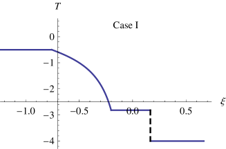
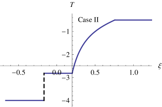
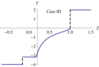
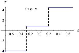
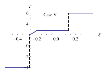
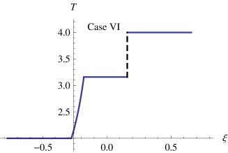
Fig. 6: Cauchy stress profiles for different locations of Riemann initial data $U_{l}$.

Case I  If $T_{r}<T_{l}<0$, the Riemann solution is $U_{l}\overset{R_{1}}{\longrightarrow}\bar{U}\overset{S_{2}}{\longrightarrow}U_{r}.$ More precisely, the solution formula is given by

$$(T,v)=\left\{\begin{array}[]{lll}(T_{l},0)&x<\xi_{1}t,\\ (\hat{T}(\xi),\hat{v}(\xi))&\xi_{1}t\leq x\leq\xi_{2}t,\\ (\bar{T},\bar{v})&\xi_{2}t<x<s_{2}t,\\ (T_{r},0)&s_{2}t<x,\end{array}\right.$$

where $\xi_{1}=-1/\sqrt{\rho\epsilon^{\prime}(T_{l})},\xi_{2}=-1/\sqrt{\rho\epsilon^{\prime}(\bar{T})}$ and $(\hat{T}(\xi),\hat{v}(\xi))$ is determined by

$$\xi=-\frac{1}{\sqrt{\rho\epsilon^{\prime}(\hat{T}(\xi))}},\quad\hat{v}(\xi)=\int_{T_{l}}^{\hat{T}}\sqrt{\frac{\epsilon^{\prime}(\tau)}{\rho}}\,d\tau.$$ (33)

In addition, by the argument in Section 2, we calculate the intermediate state $(\bar{T},\bar{v})$ via

$$\bar{v}=\int_{T_{l}}^{\bar{T}}\sqrt{\frac{\epsilon^{\prime}(\tau)}{\rho}}\,d\tau,\quad\bar{v}+\sqrt{(\bar{T}-T_{r})[\epsilon(\bar{T})-\epsilon(T_{r})]/\rho}=0,$$ (34)

and the speed of forward shock is

$$s_{2}=\frac{1}{\sqrt{\rho\frac{\epsilon(T_{r})-\epsilon(\bar{T})}{T_{r}-\bar{T}}}}.$$ (35)

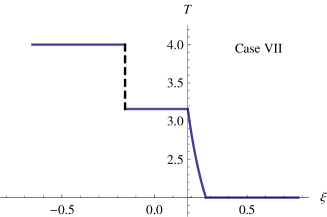
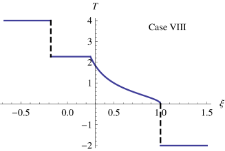
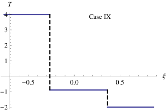
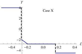
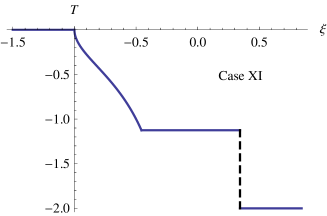
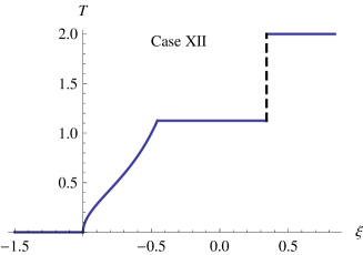
Fig. 7: Cauchy stress profiles for different locations of Riemann initial data $U_{l}$ (Continued).

It is easy to observe that if the strain-stress relation is linear, then there is no rarefaction wave (cf. (33)). Moreover, it follows from the first equation in (33) and Eq. (35) that $\xi_{1}=\xi_{2}=\lambda_{1},s_{2}=\lambda_{2}$. By (34), we further have

$$(\bar{T},\bar{v})=\left(\frac{1}{2}\left(T_{r}+T_{l}\right),\frac{1}{2}\sqrt{\frac{\alpha+\beta}{\rho}}(T_{r}-T_{l})\right).$$

So it is noted that all these results are consistent with the solution (32).

Case II  If $T_{l}<T_{r}\leq 0$, the Riemann solution is $U_{l}\overset{S_{1}}{\longrightarrow}\bar{U}\overset{R_{2}}{\longrightarrow}U_{r}.$

Case III  If $0<T_{r}<T_{*}$, the Riemann solution is $U_{l}\overset{S_{1}}{\longrightarrow}\bar{U}\overset{R_{2}}{\longrightarrow}(0,v_{*})\xrightarrow[s_{2}=\lambda_{2}(0)]{S_{2}}U_{r}.$

Case IV  If $T_{*}\leq T_{r}\leq T_{**}$, the Riemann solution is $U_{l}\overset{S_{1}}{\longrightarrow}\bar{U}\overset{S_{2}}{\longrightarrow}U_{r},$

Case V  If $T_{**}<T_{r}$, the Riemann solution is $U_{l}\xrightarrow[s_{1}=\lambda_{1}(T_{2})]{S_{1}}U_{B}\overset{R_{1}}{\longrightarrow}\bar{U}\overset{S_{2}}{\longrightarrow}U_{r}.$

Case VI  If $T_{r}>T_{l}>0$, the Riemann solution is $U_{l}\overset{R_{1}}{\longrightarrow}\bar{U}\overset{S_{2}}{\longrightarrow}U_{r}.$

Case VII  If $0\leq T_{r}<T_{l}$, the Riemann solution is $U_{l}\overset{S_{1}}{\longrightarrow}\bar{U}\overset{R_{2}}{\longrightarrow}U_{r}.$

Case VIII  If $-T_{l}=\hat{T}_{*}<T_{r}<0$, the Riemann solution is $U_{l}\overset{S_{1}}{\longrightarrow}\bar{U}\overset{R_{2}}{\longrightarrow}(0,v_{*})\xrightarrow[s_{2}=\lambda_{2}(0)]{S_{2}}U_{r}.$

Case IX  If $\hat{T}_{**}\leq T_{r}\leq\hat{T}_{*}=-T_{l}$, the Riemann solution is $U_{l}\overset{S_{1}}{\longrightarrow}\bar{U}\overset{S_{2}}{\longrightarrow}U_{r}.$

Case X  If $T_{r}<\hat{T}_{**}$, the Riemann solution is $U_{l}\xrightarrow[s_{1}=\lambda_{1}(T_{3})]{S_{1}}U_{C}\overset{R_{1}}{\longrightarrow}\bar{U}\overset{S_{2}}{\longrightarrow}U_{r}.$

Case XI  If $T_{r}<T_{l}=0$, the Riemann solution is $U_{l}\overset{R_{1}}{\longrightarrow}\bar{U}\overset{S_{2}}{\longrightarrow}U_{r}$.

Case XII  If $T_{r}>T_{l}=0$, the Riemann solution is $U_{l}\overset{R_{1}}{\longrightarrow}\bar{U}\overset{S_{2}}{\longrightarrow}U_{r}$.

In summary, there are in total twelve wave patterns depending on the initial stresses, while for a classical linearly elastic material there is only one wave pattern. Thus, if this case is realized in an experiment, by measuring the wave patterns one can determine whether the material is a classical one or the one which belongs to the sub-class of new elastic bodies defined through equation (4).

References

- [1] R. Abeyaratne, J. K. Knowles, Evolution of phase transitions: a continuum theory. Cambridge, New York, 2006.
- [2] F. Ancona, A. Marson, Sharp convergence rate of the Glimm scheme for general nonlinear hyperbolic systems, Comm. Math. Phys., 302 (2011), pp. 581-630.
- [3] S. Bianchini, A. Bressan, Vanishing viscosity solutions of nonlinear hyperbolic systems, Annals of Mathematics, 161 (2005), pp. 223-342.
- [4] M. Bulicek, J. Malek, K. R. Rajagopal and E. Suli, Elastic solids with limiting strain: modelling and analysis, EMS surveys in mathematical sciences, 1 (2014), pp. 283-332.
- [5] T. Chang, L. Hsiao, The Riemann problem and interaction of waves in gas dynamics. In Pitman Monographs and Surveys in Pure and Applied Mathematics, vol. 41. Harlow, UK: Longman Scientific and Technical and New York, NY: John Wiley & Sons Inc, 1989.
- [6] Y. C. Chen, D. C. Lagoudas, Impact induced phase transformation in shape memory alloys, Journal of the Mechanics and Physics of Solids, 48 (2000), pp. 275-300.
- [7] C. M. Dafermos, Structure of solutions of the Riemann problem for hyperbolic systems of conservation laws, Arch. Rational Mech. Anal., 53 (1974), pp. 203-217.
- [8] C. M. Dafermos, Hyperbolic conservation laws in continuum physics, Third edition. Grundlehren der Mathematischen Wissenschaften, vol. 325. Springer Verlag, Berlin, 2010.
- [9] J. Glimm, Solution in the large for nonlinear hyperbolic systems of equations, Comm. Pure Appl. Math. 18 (1965), 697-715.
- [10] S. J. Huang, H. H. Dai, and D. X. Kong, Global structure stability for the wave catching-up phenomenon in a prestressed two-material bar, SIAM J. Appl. Math., 75 (2015), pp. 585-604.
- [11] S. J. Huang, H. H. Dai, Z. Chen, and D. X. Kong, Mathematical theory and analytical solutions for the wave catching-up phenomena in a nonlinearly elastic composite bar, Proc. R. Soc. A, 468(2012), pp. 3882-3901.
- [12] K. Kannan, K. R. Rajagopal, G. Saccomandi, Unsteady motions of a new class of elastic solids, Wave motion, 51(2014), pp. 833-843.
- [13] J. K. Knowles, Impact-induced tensile waves in a rubberlike material, SIAM J. Appl. Math., 62(2002), pp. 1153-1175.
- [14] V. Kulvait, J. Mlek, and K.R. Rajagopal, Anti-plane stress state of a plate with a V-notch for a new class of elastic solids, Int. J. Fract., 179(2013), pp. 59-73.
- [15] P. D. Lax, Hyperbolic systems of conservation laws II, Comm. Pure Appl. Math. 10 (1957), pp. 537-556.
- [16] P. G. LeFloch, M. D. Thanh, Nonclassical Riemann solvers and kinetic relations I. A nonconvex hyperbolic model of phase transitions, Z. angew. Math. Phys., 52(2001), pp. 597-619.
- [17] P. G. LeFloch, Hyperbolic systems of conservation laws. The theory of classical and nonclassical shock waves, Birkhuser-Verlag, Basel, 2002.
- [18] T. P. Liu, The Riemann problem for general conservation laws, Transactions of the American Mathematical Society, 199 (1974), pp. 89-112.
- [19] T. P. Liu, The Riemann problem for general systems of conservation laws, Journal of Differential Equations, 18(1975), pp. 218-234.
- [20] X. M. Liu, Z. Wang, The Riemann problem for the nonlinear degenerate wave equations, Acta Mathematica Scientia, 31B(2011), pp. 2313-2322.
- [21] A. Matsumura and M. Mei, Nonlinear stability of viscous shock profile for a non-convex system of viscoelasticity, Osaka J. Math., 34(1997), pp. 589-603.
- [22] K. Nishihara, Stability of travelling waves with degenerate shock condition for onedimensional viscoelastic model, J. Differential Equations, 120(1995), pp. 304-318.
- [23] K. R. Rajagopal, On implicit constitutive theories, Appl. Math., 48(2003), pp. 279-319.
- [24] K. R. Rajagopal, The elasticity of elasticity, Z. Angew. Math. Phys., 58(2007), pp. 309-317.
- [25] K. R. Rajagopal, Conspectus of concepts of elasticity, Math. Mech. Solids, 16(2011), pp. 536-562.
- [26] K. R. Rajagopal, On the nonlinear elastic response of bodies in the small strain range, Acta Mech., 225(2014), pp. 1545-1553.
- [27] K. R. Rajagopal and J. Walton, Modeling fracture in the context of strain-limiting theory of elasticity, Int. J. Fract., 169(2011), pp. 39-48.
- [28] T. Saito, T. Furuta, J.H. Hwang, S. Kuramoto, K. Nishino, N. Suzuki, R. Chen, A. Yamada, K. Ito, Y. Seno, T. Nonaka, H. Ikehata, N. Nagasako, C. Iwamoto, Y. Ikuhara, and T. Sakuma, Multifunctional alloys obtained via a dislocation-free plastic deformation mechanism. Science, 300(2003), pp. 464-467.
- [29] J. Smoller, Shock waves and reaction-diffusion equations, Springer-Verlag, New York, 1994.
- [30] W. H. Sun, W. C. Sheng, The Riemann problem for nonlinear degenerate wave equations, Appl. Math. Mech. -Engl. Ed., 31(2010), pp. 665-674.
- [31] R.J. Talling, R.J. Dashwood, M. Jackson, S. Kuramoto, and D. Dye, Determination of (c11-c12) in Ti-36Nb-2Ta-3Zr-0.3O (Wt.% ) (Gum Metal), Scr. Mater., 59(2008), pp. 669-672.
- [32] A. Tzavaras, Elastic as limit of viscoelastic response in a context of self-similar viscous limits, J. Differential Equations, 123 (1995), pp. 305-341.
- [33] B. Wendroff, The Riemann problem for materials with nonconvex equations of state I: isentropic flow, J. Math. Anal. Appl., 38(1972), pp. 454-466.
- [34] B. Wendroff, The Riemann problem for materials with nonconvex equations of state II: general form, J. Math. Anal. Appl., 38(1972), pp. 640-658.
- [35] E. Withey, M. Jin, A. Minor, S. Kuramoto, D.C. Chrzan, and J.W. Jr.. Morris, The deformation of “Gum Metal” in nanoindentation, Mater. Sci. Eng. A, 493(2008), pp. 26-32.
- [36] S.Q. Zhang, S.J. Li, M.T. Jia, Y.L. Hao, and R. Yang, Fatigue properties of a multifunctional titanium alloy exhibiting nonlinear elastic deformation behavior, Scr. Mater., 60(2009), pp. 733-736.