Maximizing Coverage Centrality via Network Design: Extended Version

Abstract

Network centrality plays an important role in many applications. Central nodes in social networks can be influential, driving opinions and spreading news or rumors. In hyperlinked environments, such as the Web, where users navigate via clicks, central content receives high traffic, becoming targets for advertising campaigns. While there is an extensive amount of work on centrality measures and their efficient computation, controlling nodes’ centrality via network updates is a more recent and challenging task. Performing minimal modifications to a network to achieve a desired property falls under the umbrella of network design problems. This paper is focused on improving the group (coverage and betweenness) centrality of a set of nodes, which is a function of the number of shortest paths passing through the set, by adding edges to the network. We introduce several variations of the problem, showing that they are NP-hard as well as APX-hard. Moreover, we present a greedy algorithm, and even faster sampling algorithms, for group centrality maximization with theoretical quality guarantees under a restricted setting and good empirical results in general for several real datasets.

I Introduction

Network design is a recent area of study focused on modifying or redesigning a network in order to achieve a desired property [8, 30]. As networks become a popular framework for modeling complex systems (e.g. VLSI, transportation, communication, society), network design provides key controlling capabilities over these systems, specially when resources are constrained. Existing work has investigated the optimization of global network properties, such as minimum spanning tree [14], shortest-path distances [16, 7, 19], diameter [6], and information diffusion-related metrics [12, 27] via a few local (e.g. vertex, edge-level) upgrades. Due to the large scale of real networks, computing a global network property becomes time-intensive. For instance, computing all-pair shortest paths in large networks is prohibitive. As a consequence, design problems are inherently challenging. Moreover, because of the combinatorial nature of these local modifications, network design problems are often NP-hard, and thus, require the development of efficient approximation algorithms.

We focus on a novel network design problem, which is improving the group centrality. Given a node $v$, its coverage centrality is the number of distinct node pairs for which a shortest path passes through $v$, whereas its betweenness centrality is the fraction of shortest paths between any distinct pair of nodes passing through $v$ [29]. The centrality of a group $X$ is a function of the shortest paths that go through members of $X$ [29]. Our goal is to maximize group centrality, for a target group of nodes, via a small number of edge additions.

As an application scenario, consider an online advertising service where advertisers can place links on a set of pages depending on user context information (see Figure 1). For instance, users navigating from travel to car related pages are likely to be interested in car rentals. Thus, the ad service can display links in a subset of pages in order to increase the number of shortest paths from travel related web-pages to car related ones via a set of pages owned by a given car rental company. The idea is to boost the traffic to the car rental pages while users browse the Web, assuming that clicks will often follow shortest paths. Once the user arrives at an advertiser’s page, the car rental company can offer targeted information to support her browsing through the automobile related content (e.g. highlighting car models often rented in a given tourist location). This problem is equivalent to optimizing the group centrality of the advertiser’s pages—for a selected set of node pairs—by adding few edges from a candidate set.

Another application scenario is a professional network, such as LinkedIn, where the centrality of some users (e.g. employees of a given company) might be increased via connection recommendations/advertising. In military settings, where networks might include adversarial elements, inducing the flow of information towards key agents can enhance communication and decision making [24]. Moreover, multiple recent approaches focus on the most probable (shortest) paths to allow scalable solutions for social influence and information propagation [13, 3]. Thus, to achieve better information propagation through a target group of nodes of interest, one might improve their shortest path based centrality.

From a theoretical standpoint, for any objective function of interest, we can define a search and a corresponding design problem. In this paper, we show that, different from its search version [29], group centrality maximization cannot be approximated by a simple greedy algorithm. Furthermore, we study several variations of the problem and show that, under two realistic constraints, the problem does allow a constant factor greedy approximation. In fact, we are able to prove that our approximation for the constrained problem is optimal, in the sense that the best algorithm cannot achieve a better approximation than the one obtained by our approach. In order to scale our greedy solution to large datasets, we also propose efficient sampling schemes, with approximation guarantees, for group centrality maximization.

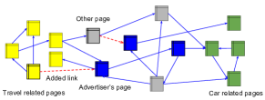
Figure 1: Application scenario: Adding links to the Web graph in order to increase user traffic from travel to car related pages via a set of car rental (advertiser’s) pages.

Our Contributions. The main contributions of this paper can be summarized as follows:

• We study several variations of a novel network design problem, the group centrality optimization, and prove that they are NP-hard as well as APX-hard.

• We propose a simple greedy algorithm and even faster sampling algorithms for group centrality maximization.

• We show the effectiveness of our algorithms on several real datasets and also prove that the proposed solutions are optimal for a constrained version of the problem.

II Problem Definition

We assume $G(V,E)$ to be an undirected graph with sets of vertices $V$ and edges $E$. A shortest path between vertices $s$ and $t$ is a path with minimum distance (in hops) among all paths between $s$ and $t$, with length $d(s,t)$. By convention, $d(s,s)=0$, for all $s\in V$. Let $P_{st}$ denote the set of vertices in the shortest paths (multiple ones might exist) between $s$ and $t$ where $s,t\notin P_{st}$. We define $Z$ as the set of candidate pairs of vertices, $Z\subseteq V\setminus X\times V\setminus X$, which we want to cover. The coverage centrality of a vertex is defined as:

$$C(v)=|\{(s,t)\in Z|v\in P_{st},s\neq v,t\neq v\}|$$ (1)

$C(v)$ gives the number of pairs of vertices with at least one shortest path going through (i.e. covered by) vertex $v$. The coverage centrality of a set of vertices $X\subseteq V$ is defined as:

$$\small C(X)=|\{(s,t)\in Z|v\in P_{st},v\in X\wedge s,t\notin X\}|$$ (2)

A set $X$ covers a pair ($s,t$) iff $X\cap P_{st}\neq\varnothing$, i.e., at least one vertex in $X$ is part of a shortest path from $s$ to $t$. Our goal is to maximize the coverage centrality of a given set $X$ over a set of pairs $Z$ by adding edges from a set of candidate edges $\Gamma$ to $G$. For instance, in our online advertising example, $X$ are pages owned by the car rental company, $Z$ are pairs of pages related to travel and cars, and $\Gamma$ are potential links that can be created to increase the traffic through the pages in $X$. Let $G_{m}$ denote the modified graph after adding edges $E_{s}\subseteq\Gamma$, $G_{m}=(V,E\cup E_{s})$. We define the coverage centrality of $X$ (over pairs in $Z$) in the modified graph $G_{m}$ as $C_{m}(X)$.

Symbols	Definitions and Descriptions
$d(s,t)$	Shortest path (s.p.) distance between $s$ and $t$
$n$	Number of nodes in the graph
$m$	Number of edges in the graph
$G(V,E)$	Given graph (vertex set $V$ and edge set $E$)
$X$	Target set of nodes
$C(v),C(X)$	Coverage centrality of node $v$, node set $X$
$\Gamma$	Candidate set of edges
$k$	budget
$P_{st}$	The set of nodes on the s.p.s between $s$ and $t$
$G_{m},C_{m}$	Modified graph and modified centrality
$Z$	Pairs of vertices to be covered
$m_{u}$	Number of uncovered pairs, $|Z|$

TABLE I: Frequently used symbols

Problem 1.

Coverage Centrality Optimization (CCO): Given a network $G=(V,E)$, a set of vertices $X\subset V$, a candidate set of edges $\Gamma$, a set of vertex pairs $Z$ and a budget $k$, find a set of edges $E_{s}\subseteq\Gamma$, such that $|E_{s}|\leq k$ and $C_{m}(X)$ is maximized.

For simplicity, in the rest of the paper, we assume $Z=V\setminus X\times V\setminus X$ unless stated otherwise. As a consequence:

$$\small C(X)=|\{(s,t)\in V\setminus X\times V\setminus X|v\in P_{st},v\in X,s<t\}|$$ (3)

where $s<t$ implies ordered pairs of vertices. Fig. 2 shows a solution for the CCO problem with budget $k=1$ for an example network where the target set $X=\{d,f\}$ and the candidate set $\Gamma=\{(d,a),(d,b),(f,b)\}$.

(a) Initial graph

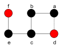
(b) Modified graph

Figure 2: Example of Coverage Centrality Optimization problem. We want to optimize the centrality of $\{d,f\}$ with a budget of one edge from the candidates $\{(d,a),(d,b),(f,b)\}$. The coverage centrality of $\{d,f\}$ is $0$ in the initial graph (a) and $3$ in the modified graph (b). Node $d$ belongs to the shortest paths between $(a,e)$, $(a,c)$ and $(a,f)$ in (b).

Similarly, we can also formulate the group betweenness centrality optimization problem. Given a vertex set $X\subseteq V$, its group betweenness centrality is defined as:

$$B(X)=\sum_{s,t\in V\setminus X}\frac{\sigma_{s,t}(X)}{\sigma_{s,t}}$$ (4)

where $\sigma_{s,t}$ is the number of shortest paths between $s$ and $t$, $\sigma_{s,t}(X)$ is the number of shortest paths between $s$ and $t$ passing through $X$. We define the group betweenness centrality of $X$ in the modified graph $G_{m}$ as $B_{m}(X)$.

Problem 2.

Betweenness Centrality Optimization (BCO): Given a network $G=(V,E)$, a node set $X\subset V$, a candidate edge set $\Gamma$, a set of node pairs $Z$ and a budget $k$, find a set of edges $E_{s}\subseteq\Gamma$, such that $|E_{s}|\leq k$ and $B_{m}(X)$ is maximized.

In this paper, we focus on the CCO problem. However, all the results described can be mapped to the BCO problem with small changes. To avoid redundancy and due to the space constraints, we omit similar results for BCO.

III Hardness and Inapproximability

This section provides complexity analysis of the CCO problem. We show that CCO is NP-hard as well as APX-hard. More specifically, CCO cannot be approximated within a factor grater than $(1-\frac{1}{e})$.

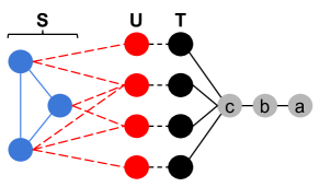
Figure 3: Example of reduction from Set Cover to Coverage Centrality Optimization, where $|U|=4$ and $|S|=3$. Target set $X=\{a\}$ and candidate edges $\Gamma$ connect $a$ to nodes in $S$.

Theorem 1.

The CCO problem is NP-hard.

Proof.

Consider an instance of the NP-complete Set Cover problem, defined by a collection of subsets $S_{1},S_{2},...,S_{m}$ for a universal set of items $U=\{u_{1},u_{2},...,u_{n}\}$. The problem is to decide whether there exist $k$ subsets whose union is $U$. To define a corresponding CCO instance, we construct an undirected graph with $m+2n+3$ nodes: there are nodes $i$ and $j$ corresponding to each set $S_{i}$ and each element $u_{j}$ respectively, and an undirected edge $(i,j)$ whenever $u_{j}\in S_{i}$. Every $S_{i}$ has an edge with $S_{j}$ when $i\neq j$ and $i,j\in{1,2,...,m}$. The set $T=\{t_{1},t_{2},...,t_{n}\}$ is a copy of set $U$ where $u_{i}$ is connected to the corresponding $t_{i}$ for all $i\in{1,2,...,n}$. Three more nodes ($a,b$ and $c$) are added to the graph where $a$ is in $X$. Node $c$ is connected to $t_{i}$ for all $i\in{1,2,...,n}$. Node $b$ is attached to $a$ and $c$. Figure 3 shows an example of this construction. The reduction clearly takes polynomial time. The candidate set $\Gamma$ consists of the edges between $a$ and set $S$. We prove that CCO of a given singleton set is NP-hard by maximizing the Coverage Centrality (CC) of the node $a$. Current CC of $a$ is $0$ by construction.

A set $S^{\prime}\subset S$, with $|S^{\prime}|\leq k$ is a set cover iff the CC of $a$ becomes $n+m+k$ after adding the edges between $a$ and every node in $S^{\prime}$. Assume that $S^{\prime}$ is a set cover and edges are added between node $a$ and every node in $S^{\prime}$. Then the CC of $a$ improves by $m+n+k$ as shortest paths between pairs $(b,s)$, $\forall s\in S$, $(b,u)$, $\forall u\in U$, and $(c,p)$, $\forall p\in S^{\prime}$, will now pass through $a$. On the other hand, assume that the CC of node $a$ is $m+n+k$ after adding edges between $a$ and any set $S^{\prime}\subset S$. It is easy to see that $m+k$ extra pairs will have their shortest paths covered by $a$. However, the only way to add another $n$ pairs is by making $S^{\prime}$ a set cover. ∎

Given that computing an optimal solution for CCO is infeasible in practice, a natural question is whether it has a polynomial-time approximation. The next theorem shows that CCO is also NP-hard to approximate within a factor greater than $(1-\frac{1}{e})$. Interestingly, different from its search counterpart [29], CCO is not submodular (see Section VII). These two results provide strong evidence that, for group centrality, network design is strictly harder than search.

Theorem 2.

CCO cannot be approximated within a factor greater than $(1-\frac{1}{e})$.

Proof.

We give an $L$-reduction [28] from the maximum coverage (MSC) problem with parameters $x$ and $y$. Our reduction is such that following two equations are satisfied:

$$OPT(I_{CCO})\leq xOPT(I_{MSC})\vspace{-2mm}$$ (5)

$$OPT(I_{MSC})-s(T^{M})\leq y(OPT(I_{CCO})-s(T^{C}))$$ (6)

where $I_{MSC}$ and $I_{CCO}$ are problem instances, and $OPT(Y)$ is the optimal value for instance $Y$. $s(T^{M})$ and $s(T^{C})$ denote any solution of the MSC and CCO instances respectively. If the conditions hold and CCO has an $\alpha$ approximation, then MSC has an $(1-xy(1-\alpha))$ approximation. However, MSC is NP-hard to approximate within a factor greater than $(1-\frac{1}{e})$. It follows that $(1-xy(1-\alpha))<(1-\frac{1}{e})$, or, $\alpha<(1-\frac{1}{xye})$ [5]. So, if the conditions are satisfied, CCO is NP-hard to approximate within a factor greater than $(1-\frac{1}{xye})$.

We use the same construction as in Theorem 1. For CCO, the set $Z$ contains pairs in the form $(b,u)$, $u\in U$. Let the solution of $I_{CCO}$ be $s(T^{C})$. The centrality of node $a$ will increase by $s(T^{C})$ to cover the pairs in $Z$. Note that $s(T^{C})=2s(T^{M})$ from the construction (as the graph is undirected, the covered pair is unordered). It follows that both the conditions are satisfied when $x=2$ and $y=\frac{1}{2}$. So, CCO is NP-hard to approximate within a factor grater than $(1-\frac{1}{e})$.

∎

Theorem 2 shows that there is no polynomial-time approximation better than $(1-\frac{1}{e})$ for CCO. Given such an inapproximation result, we propose an efficient greedy heuristic for our problem, as discussed in the next section.

IV Algorithms

IV-A Greedy Algorithm (GES)

Algorithm 1 (GES) is a simple greedy strategy that selects the best edge to be added in each of the $k$ iterations, where $k$ is the budget. Its most important steps are $2$ and $7$. In step $2$, it computes all-pair-shortest-paths in time $O(n(m+n))$. Next, it chooses, among the candidate edges $\Gamma$, the one that maximizes the marginal coverage centrality gain of $X$ (step $7$), which takes $O(|\Gamma|n^{2})$ time. After adding the best edge, the shortest path distances are updated. Then, the algorithm checks the pairwise distances in $O(n^{2})$ time (step $9$). The total running time of GES is $O(n(m+n)+k|\Gamma|n^{2})$.

0:  Network $G=(V,E)$, target node set $X$, Candidate set
of edges $\Gamma$, Budget $k$ 0:  A subset $E_{s}$ from $\Gamma$ of $k$ edges 1:  $E_{s}\leftarrow\emptyset$ 2:  Compute all pair shortest paths and store the distances 3:  while  $|E_{s}|\leq k$  do 4:     for $e\in\Gamma\setminus E_{s}$ do 5:        $\textit{Count(e)}\leftarrow$ $\#$ newly covered pairs after adding $e$ 6:     end for 7:     $e^{*}\leftarrow\operatorname*{arg\,max}_{e\in\Gamma\setminus E_{s}}\{Count(e)\}$ 8:     $E_{s}\leftarrow E_{s}\cup e^{*}$ and $E\leftarrow E\cup e^{*}$ 9:     Update the shortest path distances 10:  end while 11:  return  $E_{s}$

Algorithm 1 Greedy Edge Set (GES)

We illustrate the execution of GES on the graph from Figure 2a for a budget $k=2$, a candidate set of edges $\Gamma=\{(d,a),$ $(d,b),(f,b)\}$, and a target set $X=\{d,f\}$. Initially, adding $(d,a),(d,b)$ and $(f,b)$ increases the centrality of $X$ by $3$, $0$, and $2$, respectively, and thus $(d,a)$ is chosen. In the second iteration, $(d,b)$ and $(f,b)$ increase the centrality of $X$ by $0$ and $1$, respectively, and $(f,b)$ is chosen.

IV-B Sampling Algorithm (BUS)

The execution time of GES increases with $|\Gamma|$ and $m$. In particular, if $m=O(n^{2})$ and $|\Gamma|=O(n)$, the complexity reaches $O(n^{3})$, which is prohibitive for large graphs. To address this challenge, we propose a sampling algorithm that is nearly optimal, regarding each greedy edge choice, with probabilistic guarantees (see Section V-C). Instead of selecting edges based on all the uncovered pairs of vertices, our scheme does it based on a small number of sampled uncovered pairs. This strategy allows the selection of edges with probabilistic guarantees using a small number of samples, thus ensuring scalability to large graphs. We show that the error in estimating the coverage based on the samples is small.

Algorithm 2 (Best Edge via Uniform Sampling, or BUS) is a sampling strategy to select the best edge to be added in each of the $k$ iterations based on the sampled uncovered node pairs. For each pair of samples, we compute the distances from each node in the pair to all others. These distances estimate the number of covered pairs after the addition of one edge. In Section V-C, we provide a theoretical analysis of the approximation achieved by BUS.

The costliest steps of our algorithm are 4-7 and 8-10. Steps 4-7, where the algorithm performs shortest-path computations, take $O(q(n+m))$ time. Next, the algorithm estimates the additional number of shortest pairs covered by $X$ after adding each of the edges based on the samples (steps 8-10) in $O(|\Gamma|q^{2})$ time. Given such an estimate, the algorithm chooses the best edge to be added (step 11). The total running time of BUS is $O(kq(m+n)+k|\Gamma|q^{2})$.

0:  Network $G=(V,E)$, target node set $X$, Candidate set
of edges $\Gamma$, Budget $k$ 0:  A subset $\gamma$ from $\Gamma$ of $k$ edges 1:  Choose $q$ pairs of vertices in $Q$ from $M_{u}$ 2:  $\gamma\leftarrow\emptyset$ 3:  while  $|\gamma|\leq k$  do 4:     for  $(s,t)\in Q$  do 5:        Compute and store s.p. distance $d(s,v)$ (for all $v\in V$) 6:        Compute and store s.p. distance $d(t,v)$ (for all $v\in V$) 7:     end for 8:     for  $e\in\Gamma\setminus\gamma$ do 9:        $score_{e}\leftarrow\#$ newly covered pairs after adding $e$ 10:     end for 11:     $e^{*}\leftarrow\operatorname*{arg\,max}_{e^{\prime}\in\Gamma\setminus\gamma}\{score_{e^{\prime}}\}$ 12:     $\gamma\leftarrow\gamma\cup e^{*}$ and $E\leftarrow E\cup e^{*}$ 13:  end while 14:  Return $\gamma$

Algorithm 2 Best Edge via Uniform Sampling (BUS)

V Analysis

In the previous section, we described a greedy heuristic and an efficient algorithm to approximate the greedy approach. Next, we show, under some realistic assumptions, the described greedy algorithm provides a constant-factor approximation for a modified version of CCO. More specifically, our approximation guarantees are based on the addition of two extra constraints to the general CCO described in Section II.

V-A Constrained Problem

The extra constraints, $S^{1}$ and $S^{2}$, considered are the following: (1) $S^{1}$: We assume that edges are added from the target set $X$ to the remaining nodes, i.e. edges in a given candidate set $\Gamma$ have the form $(a,b)$ where $a\in X$ and $b\in V\setminus X$ [5]; and (2) $S^{2}$: Each pair $(s,t)$ can be covered by at most one single newly added edge [2, 19].

$S^{1}$ is a reasonable assumption in many applications. For instance, in online advertising, adding links to a third-party page gives away control over the navigation, which is undesirable. $S^{2}$ is motivated by the fact that, in real-life graphs, vertex centrality follows a skewed distribution (e.g. power-law), and thus most of the new pairs will have shortest paths through a single edge in $\Gamma$. In our experiments (see Table IV in Section VI-A), we show that, in practice, solutions for the constrained and general problem are not far from each other. Both constraints have been considered by previous work [5, 2, 19]. Next, we show that COO under constraints $S^{1}$ and $S^{2}$, or RCCO (Restricted CCO), for short, is still NP-hard.

Corollary 3.

RCCO is NP-hard.

Proof.

Follows directly from Theorem 1, as the construction applied in the proof respects both the constraints. ∎

V-B Analysis: Greedy Algorithm

The next theorem shows that RCCO’s optimization function is monotone and submodular. As a consequence, the greedy algorithm described in Section IV-A leads to a well-known constant factor approximation of $(1-1/e)$ [20].

Theorem 4.

The objective function $f(E_{s})=C_{m}(X)$ in RCCO is monotone and submodular.

Proof.

Monotonicity: Follows from the definition of a shortest path. Adding an edge $(u,v)\in E_{s}$ cannot increase $d(s,t)$ for any $(s,t)$ already covered by $X$. Since $u\in X$ for any $(u,v)\in E_{s}$, the coverage $C_{m}(X)$ is also non-decreasing.

Submodularity: We consider addition of two sets of edges, $E_{a}$ and $E_{b}$ where $E_{a}\subset E_{b}$, and show that $f(E_{a}\cup\{e\})-f(E_{a})\geq f(E_{b}\cup\{e\})-f(E_{b})$ for any edge $e\in\Gamma$ such that $e\notin E_{a}$ and $e\notin E_{b}$. Let $F(A)$ be the set of node pairs $(s,t)$ which are covered by an edge $e\in A$ ($|F(E_{s})|=C_{m}(X)$). Then $f(.)$ is submodular if $F(E_{b}\cup\{e\})\setminus F(E_{b})\subseteq F(E_{a}\cup\{e\})\setminus F(E_{a})$. To prove this claim, we make use of $S^{B}$. Therefore, each pair $(s,t)\in F(E_{b})$ is covered by only one edge in $E_{b}$. As $E_{a}\subset E_{b}$, adding $e$ to $E_{a}$ will cover some of the pairs which are already covered by $E_{b}\setminus E_{a}$. Then, for any newly covered pair $(s,t)\in F(E_{b}\cup\{e\})\setminus F(E_{b})$, it must hold that $(s,t)\in F(E_{a}\cup\{e\})\setminus F(E_{a})$. ∎

Based on Theorem 4, if $OPT$ is the optimal solution for an instance of the RCCO problem, GES will return a set of edges $E_{s}$ such that $f(E_{s})\geq(1-1/e)OPT$. The existence of such an approximation algorithm shows that the constraints $S^{1}$ and $S^{2}$ make the CCO problem easier, compared to its general version. On the other hand, whether GES is a good algorithm for the modified CCO (RCCO) remains an open question. In order to show that our algorithm is optimal, in the sense that the best algorithm for this problem cannot achieve a better approximation from those of GES, we also prove an inapproximability result for the constrained problem.

Corollary 5.

RCCO cannot be approximated within a factor greater than $(1-\frac{1}{e})$.

Proof.

Follows directly from Theorem 2, as the construction applied in the proof respects both the constraints. ∎

Corollary 5 certifies that GES achieves the best approximation possible for the constrained CCO (RCCO) problem.

V-C Analysis: Sampling Algorithm

In Section IV-B, we presented BUS, a fast sampling algorithm for the general CCO problem. Here, we study the quality of the approximation provided by BUS as a function of the number of sampled node pairs. The analysis will assume the constrained version of CCO (RCCO), but approximation guarantees regarding the general case will also be discussed.

Let us assume that $X$ covers a set $M_{c}$ of pairs of vertices. The set of remaining vertex pairs is $M_{u}$, $M_{u}=\{(s,t)|s\in V,t\in V,s\neq t,X\cap P_{st}=\emptyset\},m_{u}=|M_{u}|=n(n-1)-|M_{c}|$. We sample, uniformly with replacement, a set of ordered vertex pairs $Q$ ($|Q|=q$) from all vertex pairs ($M_{u}$) not covered by $X$. Let $g^{q}(.)$ denote the number of newly covered pairs by the candidate edges based on the samples $Q$. Moreover, for an edge set $\gamma\subset\Gamma$, let $X_{i}$ be a random variable which denotes whether the $i$th sampled pair is covered by any edge in $\gamma$. In other words, $X_{i}=1$ if the pair is covered and $0$, otherwise. Each pair is chosen with probability $\frac{1}{m_{u}}$ uniformly at random.

Lemma 1.

Given a size $q$ sample of node pairs from $M_{u}$:

$$E(g^{q}(\gamma))=\frac{q}{m_{u}}f(\gamma)$$

From the samples, we get $g^{q}(\gamma)=\Sigma_{i=1}^{q}X_{i}$. By the linearity and additive rule, $E(g^{q}(\gamma))=\Sigma_{i=1}^{q}E(X_{i})=q.E(X_{i}).$ As the probability $P(X_{i})=\frac{f(\gamma)}{m_{u}}$ and $X_{i}$s are i.i.d., $E(g^{q}(\gamma))=\frac{q}{m_{u}}f(\gamma).$ Also, let $f^{q}=\frac{m_{u}}{q}g^{q}$ be the estimated coverage.

Lemma 2.

Given $\epsilon$ $(0<\epsilon<1)$, a positive integer $l$, a budget $k$, and a sample of independent uncovered node pairs $Q,|Q|=q$, where $q(\epsilon)\geq\frac{3m_{u}(l+k)log(|\Gamma|)}{\epsilon^{2}\cdot OPT}$; then:

$$Pr(|f^{q}(\gamma)-f(\gamma)|<\epsilon\cdot OPT)\geq 1-2|\Gamma|^{-l}$$

For all $\gamma\subset\Gamma$, $|\gamma|\leq k$, where $OPT$ denotes the optimal coverage $(OPT=Max\{f(\gamma)|\gamma\subset\Gamma,|\gamma|\leq k\})$.

Proof.

Using Lemma 1:

$$\begin{split}Pr(|f^{q}(\gamma)-f(\gamma)|&\geq\delta\cdot f(\gamma))\\ Pr\Big{(}|\frac{q}{m_{u}}f^{q}(\gamma)-\frac{q}{m_{u}}f(\gamma)|&\geq\frac{q}{m_{u}}\cdot\delta\cdot f(\gamma)\Big{)}\\ Pr\Big{(}|g^{q}(\gamma)-\frac{q}{m_{u}}f(\gamma)|&\geq\frac{q}{m_{u}}\cdot\delta f(\gamma)\Big{)}\\ Pr(|g^{q}(\gamma)-E(g^{q}(\gamma))|&\geq\delta E(g^{q}(\gamma)))\end{split}$$

As the samples are independent, applying Chernoff bound:

$$Pr\Big{(}|g^{q}(\gamma)-\frac{q}{m_{u}}f(\gamma)|\geq\frac{q}{m_{u}}\delta f(\gamma)\Big{)}\leq 2\exp\Big{(}-\frac{\delta^{2}}{3}\frac{q}{m_{u}}f(\gamma)\Big{)}$$

Substituting $\delta=\frac{\epsilon OPT}{f(\gamma)}$ and $q$:

$$Pr(|f^{q}(\gamma)-f(\gamma)|\geq\epsilon\cdot OPT)\leq 2\exp\Big{(}-\frac{OPT}{f(\gamma)}(l+k)log(\Gamma)\Big{)}$$

Using the fact that $OPT\geq f(\gamma)$:

$$Pr(|f^{q}(\gamma)-f(\gamma)|\geq\epsilon\cdot OPT)\leq 2|\Gamma|^{-(l+k)}$$

Applying the union bound over all possible size-$k$ subsets of $\gamma\subset\Gamma$ (there are $|\Gamma|^{k}$) we conclude the following:

$$Pr(|f^{q}(\gamma)-f(\gamma)|\geq\epsilon\cdot OPT)<2|\Gamma|^{-l},\forall\gamma\subset\Gamma$$

$$Pr(|f^{q}(\gamma)-f(\gamma)|<\epsilon\cdot OPT)\geq 1-2|\Gamma|^{-l},\forall\gamma\subset\Gamma\qed$$

Now, we prove our main theorem which shows an approximation bound of $(1-\frac{1}{e}-\epsilon)$ by Algorithm 2 whenever the number of samples is at least $q(\epsilon/2)=\frac{12m_{u}(l+k)log(|\Gamma|)}{\epsilon^{2}\cdot OPT}$ ($l$ and $\epsilon$ are as in Lemma 2).

Theorem 6.

Algorithm 2 ensures $f(\gamma)\geq(1-\frac{1}{e}-\epsilon)OPT$ with high probability $(1-\frac{2}{|\Gamma|^{l}})$ using at least $q(\epsilon/2)$ samples.

Proof.

$f(.)$ is monotonic and submodular (Thm. 4) and one can prove the same for $f^{q}(.)$. Given the following:

1. Lemma 2: The number of samples is at least $q(\epsilon/2)$. So, with probability $1-\frac{2}{|\Gamma|^{l}}$, $f(\gamma)\geq f^{q}(\gamma)-\frac{\epsilon}{2}OPT$;

2. $f^{q}(\gamma)\geq(1-\frac{1}{e})f^{q}(\gamma*)$, $\gamma*=\operatorname*{arg\,max}_{\gamma^{\prime}\subset\Gamma,|\gamma^{\prime}|\leq k}$ $f^{q}(\gamma^{\prime})$ (submodularity property of $f^{q}(.)$);

3. $f^{q}(\gamma*)\geq f^{q}(\bar{\gamma})$, $\bar{\gamma}=\operatorname*{arg\,max}_{\gamma^{\prime}\subset\Gamma,|\gamma^{\prime}|\leq k}f(\gamma^{\prime})$ (Note that, $OPT=f(\bar{\gamma})$)

We can prove with probability $1-\frac{2}{|\Gamma|^{l}}$ that:

$$\begin{split}f(\gamma)&\geq f^{q}(\gamma)-\frac{\epsilon}{2}OPT\\ &\geq\Big{(}1-\frac{1}{e}\Big{)}f^{q}(\gamma*)-\frac{\epsilon}{2}OPT\\ &\geq\Big{(}1-\frac{1}{e}\Big{)}f^{q}(\bar{\gamma})-\frac{\epsilon}{2}OPT\\ &\geq\Big{(}1-\frac{1}{e}\Big{)}\Big{(}f(\bar{\gamma})-\frac{\epsilon}{2}OPT\Big{)}-\frac{\epsilon}{2}OPT\\ &>\Big{(}1-\frac{1}{e}-\epsilon\Big{)}OPT\qed\end{split}$$

While we are able to achieve a good probabilistic approximation with respect to the optimal value $OPT$, deciding the number of samples is not straightforward. In practice, we do not know the value of $OPT$ beforehand, which affects the number of samples needed. However, notice that $OPT$ is bounded by the number of uncovered pairs $m_{u}$. Moreover, the number of samples $q(\epsilon/2)$ depends on the ratio $\frac{m_{u}}{OPT}$. Thus, increasing this ratio while keeping the quality constant requires more samples. Also, if $OPT$ (which depends on $X$) is close to the number of uncovered pairs $m_{u}$, we need fewer samples to achieve the mentioned quality. In the experiments, we assume this ratio to be constant. Next, we propose another approximation scheme where we can reduce the number of samples by avoiding the term $OPT$ in the sample size while waiving the assumption involving constants.

Let $M_{u}$ and $m_{u}$ be the set and number of uncovered pairs by $X$ respectively in the initial graph. Let us assume,

$$\bar{q}(\epsilon)\geq\frac{3(l+k)log(|\Gamma|)}{\epsilon^{2}}$$

Corollary 7.

Given $\epsilon$ $(0<\epsilon<1)$, a positive integer $l$, a budget $k$, and a sample of independent uncovered node pairs $Q,|Q|=\bar{q}(\epsilon)$, then:

$$Pr(|f^{q}(\gamma)-f(\gamma)|<\epsilon\cdot m_{u})\geq 1-2|\Gamma|^{-l},\forall\gamma\subset\Gamma,|\gamma|\leq k$$

The proof is given in the Appendix. Next, we provide an approximation bound by our sampling scheme for at least $\bar{q}(\epsilon/2)=\frac{12(l+k)log(|\Gamma|)}{\epsilon^{2}}$ samples.

Corollary 8.

Algorithm 2 ensures $f(\gamma)\geq(1-\frac{1}{e})OPT-\epsilon.m_{u}$ with high probability $(1-\frac{2}{|\Gamma|^{l}})$ for $\bar{q}(\epsilon/2)$ samples.

Thm.	$\#$Samples	Approximations
Thm. 6	$O(\frac{m_{u}klog(|\Gamma|)}{\epsilon^{2}.OPT})$	$f(\gamma)>(1-\frac{1}{e}-\epsilon)OPT$
Cor. 8	$O(\frac{klog(|\Gamma|)}{\epsilon^{2}})$	$f(\gamma)>(1-\frac{1}{e})OPT-\epsilon.m_{u}$

TABLE II: $\#$Samples and approximations with prob. $(1-\frac{2}{|\Gamma|^{l}})$.

This proof is also in the Appendix. Table II summarizes the number of samples and corresponding bounds for Algorithm 2. Theorem 6 ensures higher quality with higher number of samples than Corollary 8. On the other hand, Corollary 8 does not assume anything about the ratio $\frac{m_{u}}{OPT}$. The results reflect a trade-off between number of samples and accuracy.

Theorem 6 and Corollary 8 assume that a greedy approach achieves a constant-factor approximation of $(1-1/e)$, which holds only for the RCCO problem (see Sections V-A and V-B). As a consequence, in the case of the general problem, the guarantees discussed in this Section apply only for each iteration of our sampling algorithm, but not for the final results. In other words, BUS provides theoretical quality guarantees that each edge selected in an iteration of the algorithm achieves a coverage within bounded distance from the optimal edge. Nonetheless, experimental results show, in practice, BUS is also effective in the general setting.

VI Experimental Results

Dataset Name	$|V|$	$|E|$
ca-GrQc (CG)	5K	14K
email-Enron (EE)	36K	183K
loc-Brightkite (LB)	58K	214K
loc-Gowalla (LG)	196K	950K
web-Stanford (WS)	280K	2.3M
DBLP (DB)	1.1M	5M

TABLE III: Dataset description and statistics.

	Ratio
Data	$k=5$	$k=10$	$k=15$
Co-authorship	$1.02$	$1.14$	$1.17$
Synthetic	$1.0$	$1.0$	$1.0$

TABLE IV: The ratio between the solutions produced by GES for the general (CCO) and constrained (RCCO) settings.

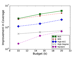
(a) Quality on CG

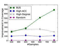
(b) Fixed Budget

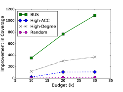
(c) Fixed $\#$Sample

Figure 4: (a) BUS vs. Greedy: Improved coverage centrality produced by different algorithms on the CG dataset. (b-c) Comparison with baselines on the EE dataset varying (b) the number of samples and (c) the budget.

Experimental Setup and Data: We evaluate the quality and scalability of our algorithms on real-world networks. All experiments were conducted on a $3.30$GHz Intel Core i7 machine with $30$ GB RAM. Algorithms were implemented in Java and all datasets applied are available online. Table III shows dataset statistics. The graphs are undirected and we consider the largest connected component for our experiments. Results reported are averages of $10$ repetitions.

We set the candidate of edges $\Gamma$ as those edges from $X$ to the remaining vertices that are absent in the initial graph (i.e. $\Gamma=\{(u,v)|u\in X\land v\in V\setminus X\land(u,v)\notin E\}$). The set of target nodes $X$ is randomly selected from the set of all nodes.

Baselines: We consider three baselines in our experiments: 1) High-ACC: Applies maximum adaptive centrality coverage [29, 17] and adds edges between target nodes $X$ and the top-$k$ centrality set; 2) High-Degree: Selects edges between the target nodes $X$ and the top $k$ high degree nodes; 3) Random: Randomly chooses $k$ edges from $\Gamma$ which are not present in the graph. We also compare our sampling algorithm (BUS) against our Greedy solution (GES) and show that BUS is more efficient while producing similar results.

VI-A GES: RCCO vs CCO

We compare coverage centrality optimization (CCO) and its restricted version (RCCO) empirically by applying GES to two small datasets: a co-authorship (NetScience) and a synthetic (Barabasi) network. The target set size $|X|$ is set to $5$. Table IV shows the ratio between results for CCO and RCCO varying the budget $k$. The results, close to $1$, provide evidence that RCCO is based on realistic assumptions.

VI-B BUS vs. GES

We apply only the smallest dataset (CG) in this experiment, as the GES algorithm is not scalable and computing all-pair-shortest-paths is required. For BUS, we set the error $\epsilon=0.3$. First, we evaluate the effect of sampling on quality, which we theoretically analyzed in Theorem 6 and Corollary 8.

Fig. 4a shows the number of new pairs covered by the algorithms. Table V shows the running times and the quality of BUS relative to the baselines—i.e. how many times more pairs are covered by BUS compared to a given baseline. BUS and GES produce results at least $2$ times better than the baselines. Moreover, BUS achieves results comparable to GES while being $2$-$3$ orders of magnitude faster.

VI-C Results for Large Graphs

We compare our sampling-based algorithm against the baseline methods using large graphs (EE, LB, LG, WS and DB). Due to the high cost of computing all-pairs shortest-paths, we estimate the coverage centrality based on $10K$ randomly selected pairs. For High-ACC, we also use sampling for adaptive coverage centrality computation [29, 17] and the same number of samples is used by High-ACC and BUS. The budget and target set size are set as $20$ and $5$, respectively.

Table VI shows the results, where the quality is relative to BUS results. BUS takes a few minutes ($8,15,17,45,85$ minutes for EE, LB, WS, LG and DB respectively) to run and significantly outperforms the baselines. This is due to the fact that existing approaches do not take into account the dependencies between the edges selected in the coverage centrality. BUS selects the edges sequentially, considering the effect of edges selected in previous steps.

	Coverage of BUS (relative to baselines)				Time [sec.]			$\#$ Samples
Budget	GES	HIgh-ACC	High-Degree	Random	GES	High-ACC	BUS	BUS
$k=10$	$1.08$	$2.46$	$5.41$	$14.45$	$>7200$	$157.1$	$5.1$	$2560$
$k=15$	$1.21$	$2.92$	$7.29$	$9.98$	$>7200$	$156.9$	$10.1$	$3840$
$k=20$	$1.29$	$2.78$	$9.96$	$9.59$	$>7200$	$157.2$	$18.2$	$5120$

TABLE V: Comparison between our sampling algorithm (BUS) and the baselines, including our Greedy (GES) approach, using the CG dataset and varying the budget $k$. We evaluate the coverage of BUS relative to the baselines—i.e. how many times more new pairs are covered by BUS compared to the baseline.

	Coverage of BUS (relative to baselines)			$\#$ Samples
Data	High-Acc	High-Degree	Random	BUS
EE	$4.88$	$2.74$	$51$	$6462$
LB	$3.3$	$2.3$	$33.8$	$6796$
LG	$3.3$	$4.2$	$62$	$4255$
WS	$1.89$	$1.95$	$4.8$	$2000$
DB	$2.5$	$1.6$	$5$	$875$

TABLE VI: BUS vs. baselines for large datasets.

VI-D Parameter Sensitivity

The main parameters of BUS are the budget and the number of samples—both affect the error $\epsilon$, as discussed in Thm. 6 and Cor. 8. We study the impact of these two parameters on performance. Again, we estimate coverage using $10K$ randomly selected pairs of nodes.

Figure 4b shows the results on EE data for budget $20$ and target set size $5$. With $600$ samples, BUS produces results at least $2$ times better than the baselines. Next, we fix the number of samples and vary the budget. Figure 4c shows the results on EE data with $10K$ samples and $5$ target nodes. BUS produces results at least $2.5$ times better than the baselines. Moreover, BUS takes only $30$ seconds to run with budget of $30$ and $1000$ samples. We find that the running time grows linearly with the budget for a fixed number of samples. These results validate the running time analysis from Section IV-B.

	Influence			Distance			Closeness
$k$	EE	LB	LG	EE	LB	LG	EE	LB	LG
$25$	$57.7$	$12.2$	$10.7$	$2.7$	$1.2$	$2.2$	$2.0$	$2.0$	$1.0$
$50$	$96.8$	$17.5$	$92.7$	$3.8$	$3.5$	$3.3$	$4.9$	$3.9$	$4.0$
$75$	$134.3$	$29.1$	$45.9$	$5.2$	$2.1$	$2.3$	$5.9$	$2.3$	$1.9$

TABLE VII: Improvement of other metrics after adding the edges found by BUS: the numbers are improvement in percentage with respect to the value for the initial graph.

VI-E Impact on other Metrics

While this paper is focused on optimizing Coverage Centrality, it is interesting to analyze how our methods affect other relevant metrics. Here, we look at the following ones: 1) influence, 2) average shortest-path distance, and 3) closeness centrality. The idea is to assess how BUS improves the influence of the target nodes, decreases the distances from the target to the remaining nodes, and increases the closeness centrality of these nodes as new edges are added to the graph. For influence analysis, we consider the popular independent cascade model [11] assuming edge probabilities as $0.1$. In all the experiments, we fix the number of sampled pairs at $1000$ and choose $10$ nodes, uniformly at random, as the target set $X$. The metrics are computed before and after the addition of edges and presented as the relative improvement in percentage. Notice that because target nodes are chosen at random, increasing the budget does not necessarily lead to an increase in the metrics considered.

Results are presented in Table VII. There is a significant improvement of the three metrics as the budget ($k$) increases. For influence, the number of seed nodes is small, and thus the relative improvement for increasing $k$ is large. The improvement of the other metrics is also significant. For instance, in EE, the decrease in distance is nearly $5\%$, which is approximately $72K$, for a budget of $75$.

VII Towards More General Settings

We start by extending our approaches to solve the Coverage Centrality optimization problem on directed graphs (e.g. our motivating example in Figure 1). In this setting, edges are added from or towards the target nodes $X$—i.e. directed edges in $\Gamma$ are of the form $(u,v)$ or $(v,u)$ where $u\in V\setminus X,v\in X$.

Problem 3.

Coverage Centrality Optimization in Directed Graphs (CCO-D): Given a directed network $G=(V,E)$, a node set $X\subset V$, a candidate edge set $\Gamma$, and a budget $k$, find edges $E_{s}\subset\Gamma$, such that $|E_{s}|\leq k$ and $C_{m}(X)$ is maximized.

We assume the same constraint $S^{2}$ for CCO-D. The next theorem shows an inapproximability result for this problem.

Theorem 9.

CCO-D under $S^{2}$ cannot be approximated within a factor greater than $(1-\frac{1}{e})$.

Proof.

We give a $L$-reduction [28] from the maximum coverage (MSC) problem with parameters $x$ and $y$. Our reduction is such that following two equations are satisfied:

$$OPT(I_{CD})\leq xOPT(I_{MSC})\vspace{-2mm}$$ (7)

$$OPT(I_{MSC})-s(T^{M})\leq y(OPT(I_{CD})-s(T^{C}))$$ (8)

where $I_{MSC}$ and $I_{CD}$ are the two problem instances, $OPT$ denotes the optimal values of the optimization problem instances. $s(T^{M})$ and $s(T^{C})$ denote any solution of the MSC and CCO-D instances respectively. If the conditions hold and CCO-D has an $\alpha$ approximation, then MSC has an $(1-xy(1-\alpha))$ approximation algorithm. However, MSC is NP-hard to approximate within a factor greater than $(1-\frac{1}{e})$. It follows that $(1-xy(1-\alpha))<(1-\frac{1}{e})$, or, $\alpha<(1-\frac{1}{xye})$ [5]. So, if the above two conditions are satisfied then CCO-D is NP-hard to approximate within a factor greater than $(1-\frac{1}{xye})$.

Consider an instance of the Maximum Coverage (MSC) problem, defined by a collection of subsets $S_{1},S_{2},...,S_{m}$ for a universal set of items $U=\{u_{1},u_{2},...,u_{n}\}$. To define a corresponding CCO-D instance, we construct an directed graph with $m+n+3$ nodes: there are nodes $i$ and $j$ corresponding to each set $S_{i}$ and each element $u_{j}$ respectively, and an directed edge $(i,j)$ whenever $u_{j}\in S_{i}$. Three more nodes ($a,b$ and $c$) are added to the graph where $a$ is in $X$. Node $c$ is connected to $u_{i}$ by $(c,u_{i})$ for all $i\in{1,2,...,n}$. Node $b$ is attached to $a$ by $(b,a)$ and $c$ by $(b,c)$. Figure 5 shows an example of this construction. The reduction clearly takes polynomial time. The candidate set $\Gamma$ consists of the edges between $a$ and the set $S$. For CCO-D, the set to be covered, $Z$ contains pairs in the form $(b,u)$ where $u\in U$.

Let the solution of $I_{CD}$ be $s(T^{C})$. The centrality of $a$ will increase by $s(T^{C})$ to cover the pairs in $Q$. Note that $s(T^{C})=s(T^{M})$ by construction. It follows that both the conditions are satisfied when $x=y=1$. So, CCO-D is NP-hard to approximate within a factor grater than $(1-\frac{1}{e})$. ∎

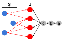
Figure 5: Example of reduction from Maximum Set Coverage, where $|U|=4$ and $|S|=3$. Target set $X=\{a\}$ and candidate edges $\Gamma$ connect $a$ to nodes in set $S$.

The next theorem shows that the objective function associated with Problem 3 under $S^{2}$ is also monotone and submodular, as was the case for the undirected setting.

Theorem 10.

Given $X$, the objective function, $f(E_{s})=C_{m}(X)$ in CCO-D is monotone and submodular.

The proof for Theorem 10 is similar to that for Theorem 4. Based on this Theorem, our algorithm (BUS) can be applied to solve CCO-D with similar guarantees. In other words, our approach is agnostic to the direction of edges. Interestingly, Theorem 9 and Theorem 10 certify that GES achieves the best approximation for the constrained CCO-D problem.

We also briefly discuss group centrality optimization under different settings. In particular, we focus on possible restrictions on the set of candidate edges $\Gamma$. For undirected graphs, $S^{0}$: $\Gamma$ is a subset of the set of absent edges, $S^{1}$: $\Gamma$ consists of absent edges of the form $(u,v)$ where either $u$ or $v$ belongs to the target set $X$, and $S^{2}$: a pair is covered using at most one newly added edge. For directed graphs, $S^{3}$: $\Gamma$ is a subset of the set of absent edges with arbitrary direction and $S^{4}$: $\Gamma$ consists of absent edges of the form $(u,v)$ where either $u$ or $v$ belongs to $X$, with any direction. The hardness of these problems can be assessed with variations of the reasoning applied in Theorem 1. Table VIII summarizes the different problem settings. We have already proven that the objective function is submodular for $S^{1}$ and $S^{2}$ (undirected) and for $S^{4}$ and $S^{2}$ (directed). Additionally, we prove that the objective functions for $S^{1}$ and $S^{4}$ individually are not submodular.

	Undirected			Directed
Settings	$S^{0}$	$S^{1}$	$S^{1}$, $S^{2}$	$S^{3}$	$S^{4}$	$S^{4}$,$S^{2}$
Submodularity	No	No	Yes	No	No	Yes

TABLE VIII: Summary of CCO under different settings.

Non-submodularity under $S^{1}$ and $S^{4}$: Counterexamples are shown in Fig. 6. For $S^{1}$: Consider $T=\{(x,a)\},S=\{\},e=(x,b)$ and a target node $x$. Clearly, $S\subset T$ and $f(T)=f(S)=0$. But $f(T\cup\{e\})=1$ as $x$ is covering $(a,b)$, whereas $f(S\cup\{e\})=0$. So, $f(T\cup\{e\})-f(T)>f(S\cup\{e\})-f(S)$, and, $f$ is not submodular. For $S^{4}$: The proof is similar to $S^{1}$. Let $T=\{(a,x)\},S=\{\},e=(x,b)$ and the target node be $x$. Thus, $S\subset T$ and $f(T)=f(S)=0$. But $f(T\cup\{e\})=1$ as $x$ is covering $(a,b)$, whereas $f(S\cup\{e\})=0$. So, $f(T\cup\{e\})-f(T)>f(S\cup\{e\})-f(S)$ and $f$ is not submodular.

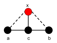
(a) Undirected, $S^{1}$

(b) Directed, $S^{4}$

Figure 6: Non-submodularity under (a) $S^{1}$ and (b) $S^{4}$.

VIII Previous Work

There is a considerable amount of work on network design targeting various objectives by modifying the network structure and node/edge attributes.

General network design problems: A set of design problems were introduced by Paik et al. [21]. They focused on vertex upgrades to improve the delays on adjacent edges. Krumke et al. [14] generalized this model and proposed minimizing the cost of the minimum spanning tree with varying upgrade costs for vertices/edges. Lin et al. [16] also proposed a shortest path optimization problem via improving edge weights under a budget constraint and with undirected edges. In [7, 18], the authors studied a different version of the problem, where weights are set to the nodes.

Design problems via edge addition: Meyerson et al. [19] proposed approximation algorithms for single-source and all-pair shortest paths minimization. Faster algorithms for the same problems were presented in [22]. Demaine et al. [6] minimized the diameter of a network and node eccentricity by adding shortcut edges with a constant factor approximation algorithm. Past research had also considered eccentricity minimization in a composite network [24]. However, all aforementioned problems are based on improving distances and hence are complementary to our objective.

Centrality computation and related optimization problems: This line of research is the most related to the present work. The first efficient algorithm for betweenness centrality computation was proposed by Brandes [1]. Recently, [25] introduced an approach for computing the top-$k$ nodes in terms of betweenness centrality via VC-dimension theory. Yoshida [29] studied similar problems —for both betweenness and coverage centrality— in the adaptive setting, where shortest paths already covered by selected nodes are not taken into account. Yoshida’s algorithm was later improved using a different sampling scheme [17]. Here, we focus on the design version of the problem, where the goal is to optimize the coverage centrality of a target set of nodes by adding edges. When the target set has size one, optimization of different centralities was studied in [5, 10]. In [23], the authors solved a similar problem, which is maximizing the expected decrease in the sum of the shortest paths from a single source to the remaining nodes via edge addition.

IX Conclusions

In this paper, we studied several variations of a novel network design problem, the group centrality optimization. This general problem has applications in a variety of domains including social, collaboration, and communication networks. From a computational hardness perspective, we have shown that the variations of problem are NP-hard as well as APX-hard. Moreover, we have proposed a simple greedy algorithm, and even faster sampling algorithms, for group centrality optimization. Our algorithms provide theoretical quality guarantees under realistic constrained versions of the problem and also outperform the baseline methods by up $5$ times in real datasets. While we have focused our discussion on coverage centrality, our results also generalize to betweenness centrality. From a broader point of view, we believe that this paper highlights interesting properties of network design problems compared to their standard search counterparts.

As future work, we will investigate the dynamic version of the problem [9, 15, 26], where coverage centrality has to be maintained under temporal, and possibly adversarial, edge updates. This problem has interesting connections with existing work on Game Theory [4]. Moreover, we will study other design problems that optimize social influence and consensus in networks [12, 2].

Appendix

Proof of Corollary 7
Using Lemmas 1 and 2:

$$\begin{split}Pr(|f^{q}(\gamma)-f(\gamma)|&\geq\delta\cdot f(\gamma))\\ Pr(|g^{q}(\gamma)-E(g^{q}(\gamma))|&\geq\delta E(g^{q}(\gamma)))\end{split}$$

The rest of the proof follows that for Lemma 2 but replacing $OPT$ by $m_{u}$. As the samples are independent, we can apply the Chernoff bound:

$$Pr\Big{(}|g^{q}(\gamma)-\frac{\bar{q}}{m_{u}}f(\gamma)|\geq\frac{\bar{q}}{m_{u}}\delta f(\gamma)\Big{)}\leq 2\exp\Big{(}-\frac{\delta^{2}}{3}\frac{\bar{q}}{m_{u}}f(\gamma)\Big{)}$$

Now, substituting $\delta=\frac{\epsilon\cdot m_{u}}{f(\gamma)}$ and $\bar{q}$:

$$Pr(|f^{q}(\gamma)-f(\gamma)|\geq\epsilon\cdot m_{u})\leq 2\exp\Big{(}-\frac{m_{u}}{f(\gamma)}(l+k)log(\Gamma)\Big{)}$$

Using the fact that $m_{u}\geq f(\gamma)$:

$$Pr(|f^{q}(\gamma)-f(\gamma)|\geq\epsilon m_{u})\leq 2|\Gamma|^{-(l+k)}$$

Now, we apply the union bound over all possible size-$k$ subsets of $\gamma\subset\Gamma$ (there are $|\Gamma|^{k}$) to get the following:

$$Pr(|f^{q}(\gamma)-f(\gamma)|\geq\epsilon\cdot m_{u})<2|\Gamma|^{-l},\forall\gamma\subset\Gamma$$

$$Pr(|f^{q}(\gamma)-f(\gamma)|<\epsilon\cdot m_{u})\geq 1-2|\Gamma|^{-l},\forall\gamma\subset\Gamma$$

Proof of Corollary 8
By the same arguments as in the proof of Theorem 6, with probability $1-\frac{2}{|\Gamma|^{l}}$:

$$\begin{split}f(\gamma)&\geq f^{q}(\gamma)-\frac{\epsilon}{2}m_{u}\\ &\geq\Big{(}1-\frac{1}{e}\Big{)}f^{q}(\gamma*)-\frac{\epsilon}{2}m_{u}\\ &\geq\Big{(}1-\frac{1}{e}\Big{)}f^{q}(\bar{\gamma})-\frac{\epsilon}{2}m_{u}\\ &\geq\Big{(}1-\frac{1}{e}\Big{)}\Big{(}f(\bar{\gamma})-\frac{\epsilon}{2}M_{u}\Big{)}-\frac{\epsilon}{2}m_{u}\\ &=\Big{(}1-\frac{1}{e}\Big{)}OPT-\Big{(}\epsilon-\frac{\epsilon}{2e}\Big{)}m_{u}\\ &>\Big{(}1-\frac{1}{e}\Big{)}OPT-\epsilon m_{u}\end{split}$$

References

- [1] U. Brandes. A faster algorithm for betweenness centrality. Journal of mathematical sociology, pages 163–177, 2001.
- [2] V. Chaoji, S. Ranu, R. Rastogi, and R. Bhatt. Recommendations to boost content spread in social networks. In WWW, pages 529–538, 2012.
- [3] W. Chen, C. Wang, and Y. Wang. Scalable influence maximization for prevalent viral marketing in large-scale social networks. In KDD, pages 1029–1038. ACM, 2010.
- [4] E. N. Ciftcioglu, S. Pal, K. S. Chan, D. H. Cansever, A. Swami, A. Singh, and P. Basu. Topology design under adversarial dynamics. In WiOpt, pages 1–8. IEEE, 2016.
- [5] P. Crescenzi, G. D’Angelo, L. Severini, and Y. Velaj. Greedily improving our own centrality in a network. In SEA, pages 43–55. Springer International Publishing, 2015.
- [6] E. D. Demaine and M. Zadimoghaddam. Minimizing the diameter of a network using shortcut edges. SWAT, ser. Lecture Notes in Computer Science, H. Kaplan,Ed., pages 420–431, 2010.
- [7] B. Dilkina, K. J. Lai, and C. P. Gomes. Upgrading shortest paths in networks. In Integration of AI and OR Techniques in Constraint Programming for Combinatorial Optimization Problems, pages 76–91. Springer, 2011.
- [8] A. Gupta and J. Könemann. Approximation algorithms for network design: A survey. Surveys in Operations Research and Management Science, pages 3–20, 2011.
- [9] T. Hayashi, T. Akiba, and Y. Yoshida. Fully dynamic betweenness centrality maintenance on massive networks. Proceedings of the VLDB Endowment, 9(2):48–59, 2015.
- [10] V. Ishakian, D. Erdos, E. Terzi, and A. Bestavros. A framework for the evaluation and management of network centrality. In SDM, pages 427–438. SIAM, 2012.
- [11] D. Kempe, J. Kleinberg, and É. Tardos. Maximizing the spread of influence through a social network. In KDD, pages 137–146, 2003.
- [12] E. B. Khalil, B. Dilkina, and L. Song. Scalable diffusion-aware optimization of network topology. In KDD, pages 1226–1235. ACM, 2014.
- [13] M. Kimura and K. Saito. Tractable models for information diffusion in social networks. In PKDD, pages 259–271, 2006.
- [14] S. Krumke, M. Marathe, H. Noltemeier, R. Ravi, and S. Ravi. Approximation algorithms for certain network improvement problems. Journal of Combinatorial Optimization, 2:257–288, 1998.
- [15] K. Lerman, R. Ghosh, and J. H. Kang. Centrality metric for dynamic networks. In Proceedings of the Eighth Workshop on Mining and Learning with Graphs, pages 70–77. ACM, 2010.
- [16] Y. Lin and K. Mouratidis. Best upgrade plans for single and multiple source-destination pairs. GeoInformatica, 19(2):365–404, 2015.
- [17] A. Mahmoody, E. Charalampos, and E. Upfal. Scalable betweenness centrality maximization via sampling. In KDD. ACM, 2016.
- [18] S. Medya, P. Bogdanov, and A. Singh. Towards scalable network delay minimization. In ICDM, pages 1083–1088. IEEE, 2016.
- [19] A. Meyerson and B. Tagiku. Minimizing average shortest path distances via shortcut edge addition. In APPROX-RANDOM, I. Dinur, K.Janson, J.Noar and J. D. P. Rolim Eds, Vol. 5687. Springer, pages 272–285, 2009.
- [20] G. L. Nemhauser, L. A. Wolsey, and M. L. Fisher. Best algorithms for approximating the maximum of a submodular set function. Math. Oper. Res., pages 177–188, 1978.
- [21] D. Paik and S. Sahni. Network upgrading problems. Networks, pages 45–58, 1995.
- [22] N. Parotisidis, E. Pitoura, and P. Tsaparas. Selecting shortcuts for a smaller world. In SDM, pages 28–36. SIAM, 2015.
- [23] N. Parotsidis, E. Pitoura, and P. Tsaparas. Centrality-aware link recommendations. In WSDM, pages 503–512. ACM, 2016.
- [24] S. Perumal, P. Basu, and Z. Guan. Minimizing eccentricity in composite networks via constrained edge additions. In MILCOM, pages 1894–1899, 2013.
- [25] M. Riondato and E. M. Kornaropoulos. Fast approximation of betweenness centrality through sampling. In WSDM, pages 413–422. ACM, 2014.
- [26] T. Takaguchi, Y. Yano, and Y. Yoshida. Coverage centralities for temporal networks. The European Physical Journal B, 89(2):1–11, 2016.
- [27] H. Tong, B. A. Prakash, T. Eliassi-Rad, M. Faloutsos, and C. Faloutsos. Gelling, and melting, large graphs by edge manipulation. In CIKM, pages 245–254. ACM, 2012.
- [28] D. P. Williamson and D. B. Shmoys. The design of approximation algorithms. Cambridge university press, 2011.
- [29] Y. Yoshida. Almost linear-time algorithms for adaptive betweenness centrality using hypergraph sketches. In KDD, pages 1416–1425. ACM, 2014.
- [30] Q. K. Zhu. Power distribution network design for VLSI. John Wiley & Sons, 2004.