Constraint Answer Set Solver EZCSP and Why Integration Schemas Matter

Abstract

Researchers in answer set programming and constraint programming have spent significant efforts in the development of hybrid languages and solving algorithms combining the strengths of these traditionally separate fields. These efforts resulted in a new research area: constraint answer set programming. Constraint answer set programming languages and systems proved to be successful at providing declarative, yet efficient solutions to problems involving hybrid reasoning tasks. One of the main contributions of this paper is the first comprehensive account of the constraint answer set language and solver ezcsp, a mainstream representative of this research area that has been used in various successful applications. We also develop an extension of the transition systems proposed by Nieuwenhuis et al. in 2006 to capture Boolean satisfiability solvers. We use this extension to describe the ezcsp algorithm and prove formal claims about it. The design and algorithmic details behind ezcsp clearly demonstrate that the development of the hybrid systems of this kind is challenging. Many questions arise when one faces various design choices in an attempt to maximize system’s benefits. One of the key decisions that a developer of a hybrid solver makes is settling on a particular integration schema within its implementation. Thus, another important contribution of this paper is a thorough case study based on ezcsp, focused on the various integration schemas that it provides.
Under consideration in Theory and Practice of Logic Programming (TPLP).

1 Introduction

Knowledge representation and automated reasoning are areas of Artificial Intelligence dedicated to understanding and automating various aspects of reasoning. Such traditionally separate fields of AI as answer set programming (ASP) Niemelä (1999); Marek and Truszczyński (1999); Brewka et al. (2011), propositional satisfiability (SAT) Gomes et al. (2008), constraint (logic) programming (CSP/CLP) Rossi et al. (2008); Jaffar and Maher (1994) are all representatives of distinct directions of research in automated reasoning. The algorithmic techniques developed in subfields of automated reasoning are often suitable for distinct reasoning tasks. For example, ASP proved to be an effective tool for formalizing elaborate planning tasks, whereas CSP/CLP is efficient in solving difficult scheduling problems. However, when solving complex practical problems, such as scheduling problems involving elements of planning or defeasible statements, methods that go beyond traditional ASP and CSP are sometimes desirable. By allowing one to leverage specialized algorithms for solving different parts of the problem at hand, these methods may yield better performance than the traditional ones. Additionally, by allowing the use of constructs that more closely fit each sub-problem, they may yield solutions that conform better to the knowledge representation principles of flexibility, modularity, and elaboration tolerance. This has led, in recent years, to the development of a plethora of hybrid approaches that combine algorithms and systems from different AI subfields. Constraint logic programming Jaffar and Maher (1994), satisfiability modulo theories (SMT) Nieuwenhuis et al. (2006), HEX-programs Eiter et al. (2005), and VI-programs Calimeri et al. (2007) are all examples of this current. Various projects have focused on the intersection of ASP and CSP/CLP, which resulted in the development of a new field of study, often called constraint answer set programming (CASP) Elkabani et al. (2004); Mellarkod et al. (2008); Gebser et al. (2009); Balduccini (2009a); Drescher and Walsh (2011); Lierler (2014).

Constraint answer set programming allows one to combine the best of two different automated reasoning worlds: (1) the non-monotonic modeling capabilities and SAT-like solving technology of ASP and (2) constraint processing techniques for effective reasoning over non-Boolean constructs. This new area has already demonstrated promising results, including the development of CASP solvers acsolver Mellarkod et al. (2008), clingcon Gebser et al. (2009), ezcsp Balduccini (2009a), idp Wittocx et al. (2008), inca Drescher and Walsh (2011), dingo Janhunen et al. (2011), mingo Liu et al. (2012), aspmt2smt Bartholomew and Lee (2014), and ezsmt Susman and Lierler (2016). CASP opens new horizons for declarative programming applications. For instance, research by Balduccini (2011) on the design of CASP language ezcsp and on the corresponding solver, which is nowadays one of the mainstream representatives of CASP systems, yielded an elegant, declarative solution to a complex industrial scheduling problem.

Unfortunately, achieving the level of integration of CASP languages and systems requires nontrivial expertise in multiple areas, such as SAT, ASP and CSP. The crucial message transpiring from the developments in the CASP research area is the need for standardized techniques to integrate computational methods spanning these multiple research areas. We argue for undertaking an effort to mitigate the difficulties of designing hybrid reasoning systems by identifying general principles for their development and studying the implications of various design choices. Our work constitutes a step in this direction. Specifically, the main contributions of our work are:

1. The paper provides the first comprehensive account of the constraint answer set solver ezcsp Balduccini (2009a), a long-time representative of the CASP subfield. We define the language of ezcsp and illustrate its use on several examples. We also account for algorithmic and implementation details behind ezcsp.

2. To present the ezcsp algorithm and prove formal claims about the system, we develop an extension of the transition systems proposed by Nieuwenhuis et al. (2006) for capturing SAT/SMT algorithms. This extension is well-suited for formalizing the behavior of the ezcsp solver.

3. We also conduct a case study exploring a crucial aspect in building hybrid systems – the integration schemas of participating solving methods. This allows us to shed light on the costs and benefits of this key design choice in hybrid systems. For the case study, we use ezcsp as a research tool and study its performance with three integration schemas: “black-box”, “grey-box”, and “clear-box”. One of the main conclusions of the study is that there is no single choice of integration schema that achieves best performance in all cases. As such, the choice of integration schema should be made as easily configurable as it is the choice of particular branching heuristics in SAT or ASP solvers. The work on analytical and architectural aspects described in this paper shows how this can be achieved.

We begin this paper with a review of the ASP and CASP formalisms. In Section 3 we present the ezcsp language. In Section 4 we provide a broader context to our study by drawing a parallel between CASP and SMT solving. Then we review the integration schemas used in the design of hybrid solvers focusing on the schemas implemented in ezcsp. Section 5 provides a comprehensive account of algorithmic aspects of ezcsp. Section 6 introduces the details of the “integration schema” case study. In particular, it provides details on the application domains considered, namely, Weighted Sequence, Incremental Scheduling, and Reverse Folding. The section also discusses the variants of the encodings we compared. Experimental results and their analysis form Section 7. Section 8 provides a brief overview of CASP solvers. The conclusions are stated in Section 9.

Parts of this paper have been earlier presented at ASPOCP 2009 Balduccini (2009a) and at PADL 2012 Balduccini and Lierler (2012).

2 Preliminaries

2.1 Regular Programs

A regular (logic) program is a finite set of rules of the form

$$\begin{array}[]{l}a_{0}\leftarrow a_{1},\dots,a_{l},not\ a_{l\mathchar 43\relax 1},\dots,not\ a_{m},not\ not\ a_{m\mathchar 43\relax 1},\dots,not\ not\ a_{n},\end{array}$$ (1)

where $a_{0}$ is $\bot$ (false) or an atom, and each $a_{i}$ ($1\leq i\leq n$) is an atom so that $a_{i}\neq a_{j}$ ($1\leq i\mathchar 60\relax j\leq l$), $a_{i}\neq a_{j}$ ($l\mathchar 43\relax 1\leq i\mathchar 60\relax j\leq m$), and $a_{i}\neq a_{j}$ ($m\mathchar 43\relax 1\leq i\mathchar 60\relax j\leq n$). This is a special case of programs with nested expressions Lifschitz et al. (1999). The expression $a_{0}$ is the head of a rule (1). If $a_{0}\mathchar 61\relax\bot$, we often omit $\bot$ from the notation. We call such rules denials. We call the right hand side of the arrow in (1) the body. If a body of a rule is empty, we call such rule a fact and omit the $\leftarrow$ symbol. We also ignore the order of the elements in the rule. For example, rule $a\leftarrow b,c$ is considered identical to $a\leftarrow c,b$. If $B$ denotes the body of (1), we write $B^{pos}$ for the elements occurring in the positive part of the body, i.e., $B^{pos}\mathchar 61\relax\{a_{1},\dots,a_{l}\}$. We frequently identify the body of (1) with the conjunction of its elements (in which $not\ not$ is dropped and $not$ is replaced with the classical negation connective $\neg$):

$$a_{1}\wedge\dots\wedge a_{l}\wedge\neg a_{l\mathchar 43\relax 1}\wedge\dots\land\neg a_{m}\wedge a_{m\mathchar 43\relax 1}\wedge\dots\land a_{n}\mathbin{\cdot}$$ (2)

Similarly, we often interpret a rule (1) as a clause

$$a_{0}\vee\neg a_{1}\vee\dots\vee\neg a_{l}\vee a_{l\mathchar 43\relax 1}\vee\dots\vee a_{m}\vee\neg a_{m\mathchar 43\relax 1}\vee\dots\vee\neg a_{n}$$ (3)

In the case when $a_{0}\mathchar 61\relax\bot$ in (1), $a_{0}$ is absent in (3). Given a program $\Pi$, we write $\Pi^{cl}$ for the set of clauses of the form (3) corresponding to the rules in $\Pi$.

Answer sets

An alphabet is a set of atoms. The semantics of logic programs relies on the notion of answer sets, which are sets of atoms. A literal is an atom $a$ or its negation $\neg a$. We say that a set $M$ of literals is complete over alphabet $\sigma$ if, for any atom $a$ in $\sigma$, either $a\in M$ or $\neg a\in M$. It is easy to see how a set $X$ of atoms over some alphabet $\sigma$ can be identified with a complete and consistent set of literals over $\sigma$ (an interpretation):

• $\displaystyle\hskip 25.00003pt{\{a\mid a\in X\}\cup\{\neg a\mid a\in\sigma\setminus X\}\mathbin{\cdot}}$

We now restate the definition of an answer set due to Lifschitz et al. (1999) in a form convenient for our purposes. By $\mathit{At}(\Pi)$ we denote the set of all atoms that occur in $\Pi$. The reduct $\Pi^{X}$ of a regular program $\Pi$ with respect to set $X$ of atoms over $\mathit{At}(\Pi)$ is obtained from $\Pi$ by deleting each rule (1) such that $X$ does not satisfy its body (recall that we identify its body with (2)), and replacing each remaining rule (1) by $a_{0}\leftarrow B^{pos}$. A set $X$ of atoms is an answer set of a regular program $\Pi$ if it is subset minimal among the sets of atoms satisfying $(\Pi^{X})^{cl}$. For example, consider a program consisting of a single rule

$$a\leftarrow\ not\ not\ a\mathbin{\cdot}$$

This program has two answer sets: set $\emptyset$ and set $\{a\}$. Indeed, $(\Pi^{\emptyset})^{cl}$ is an empty set of clauses so that $\emptyset$ is subset minimal among the sets of atoms that satisfies $(\Pi^{\emptyset})^{cl}$. On the other hand, $(\Pi^{\{a\}})^{cl}$ consists of a single clause $a$. Set $\{a\}$ is subset minimal among the sets of atoms that satisfies $(\Pi^{\{a\}})^{cl}$.

A choice rule construct $\{a\}\leftarrow B$ Niemelä and Simons (2000) of the lparse language can be seen as an abbreviation for a rule $a\leftarrow\ not\ not\ a,B$ Ferraris and Lifschitz (2005). We adopt this abbreviation in the rest of the paper.

Example 1

Consider the regular program

$$\begin{array}[]{l}\{switch\}\mathbin{\cdot}\\ lightOn\leftarrow\ switch,not\ am\mathbin{\cdot}\\ \leftarrow not\ lightOn\mathbin{\cdot}\\ \{am\}\mathbin{\cdot}\\ \end{array}$$ (4)

Intuitively, the rules of the program state the following:

• action switch is exogenous,

• light is on only if an action switch occurs during the non-am hours,

• it is impossible that light is not on (in other words, light must be on).

• it is either the case that these are am hours or not,

This program’s only answer set is $\{switch,\ lightOn\}$.

We now state an important result that summarizes the effect of adding denials to a program. For a set $M$ of literals, by $M^{\mathchar 43\relax}$ we denote the set of positive literals in $M$. For instance, $\{a,c,\neg b\}^{\mathchar 43\relax}\mathchar 61\relax\{a,c\}$.

Theorem 1 (Proposition 2 from Lifschitz et al. (1999))

For a program $\Pi$, a set $\Gamma$ of denials, and a consistent and complete set $M$ of literals over $\mathit{At}(\Pi)$, $M^{\mathchar 43\relax}$ is an answer set of $\Pi\cup\Gamma$ if and only if $M^{\mathchar 43\relax}$ is an answer set of $\Pi$ and $M$ is a model of $\Gamma^{cl}$.

Unfounded sets

For a literal $l$, by $\overline{l}$ we denote its complement. For a conjunction (disjunction) $B$ of literals, $\overline{B}$ stands for a disjunction (conjunction) of the complements of literals. For instance, $\overline{a\wedge\neg b}\mathchar 61\relax\neg a\vee b$. We sometimes associate disjunctions and conjunctions of literals with the sets containing these literals. For example, conjunction $\neg a\wedge b$ and disjunction $\neg a\vee b$ are associated with the set $\{\neg a,\leavevmode\nobreak\ b\}$ of literals. By $Bodies(\Pi,a)$ we denote the set of the bodies of all rules of program $\Pi$ with the head $a$ (including the empty body that can be seen as $\top$).

A set $U$ of atoms occurring in a program $\Pi$ is unfounded Van Gelder et al. (1991); Lee (2005) on a consistent set $M$ of literals with respect to $\Pi$ if for every $a\in U$ and every $B\in Bodies(\Pi,a)$, $M\cap\overline{B}\not\mathchar 61\relax\emptyset$ or $U\cap B^{pos}\neq\emptyset$. We say that a consistent and complete set $M$ of literals over $\mathit{At}(\Pi)$ is a model of $\Pi$ if it is a model of ${\Pi}^{cl}$.

We now state a result that can be seen as an alternative way to characterize answer sets of a program.

Theorem 2 (Theorem on Unfounded Sets from Lee (2005))

For a program $\Pi$ and a consistent and complete set $M$ of literals over $\mathit{At}(\Pi)$, $M^{\mathchar 43\relax}$ is an answer set of $\Pi$ if and only if $M$ is a model of $\Pi$ and $M$ contains no non-empty subsets unfounded on $M$ with respect to $\Pi$.

Theorem 2 is essential in understanding key features of modern answer set solvers. It provides a description of properties of answer sets that are utilized by so called “propagators” of solvers. Section 5 relies on these properties.

2.2 Logic Programs with Constraint Atoms

A constraint satisfaction problem (CSP) is defined as a triple $\langle X,D,C\rangle$, where $X$ is a set of variables, $D$ is a domain – a (possibly infinite) set of values – and $C$ is a set of constraints. Every constraint is a pair $\langle t,R\rangle$, where $t$ is an $n$-tuple of variables and $R$ is an $n$-ary relation on $D$. When arithmetic constraints are considered, it is common to replace explicit representations of relations as collections of tuples by arithmetic expressions. For instance, for a domain of three values $\{1,2,3\}$ and binary-relation $R$ consisting of ordered pairs $(1,1),(2,2)$, and $(3,3)$, we can abbreviate the constraint $\langle x,y,R\rangle$ by the expression $x\mathchar 61\relax y$. We follow this convention in the rest of the paper.

An evaluation of the variables is a function from the set of variables to the domain of values, $\nu:X\rightarrow D$. An evaluation $\nu$ satisfies a constraint $\langle(x_{1},\ldots,x_{n}),R\rangle$ if $(v(x_{1}),\ldots,v(x_{n}))\in R$. A solution is an evaluation that satisfies all constraints.

For a constraint $c\mathchar 61\relax\langle t,R\rangle$, where $D$ is the domain of its variables and $k$ is the arity of $t$, we call the constraint $\overline{c}\mathchar 61\relax\langle t,D^{k}\setminus R\rangle$ the complement of $c$. Obviously, an evaluation of variables in $t$ satisfies $c$ if and only if it does not satisfy $\overline{c}$.

For a set $M$ of literals and alphabet $\mathcal{B}$, by $M_{|\mathcal{B}}$ we denote the set of literals over alphabet $\mathcal{B}$ in $M$. For example, $\{\neg a,\leavevmode\nobreak\ b,c\}_{|\{a,b\}}\mathchar 61\relax\{\neg a,\leavevmode\nobreak\ b\}$.

A logic program with constraint atoms (CA program) is a quadruple

• $\displaystyle\hskip 25.00003pt{\langle\Pi,\mathcal{C},\gamma,D\rangle,}$

where

• $\mathcal{C}$ is an alphabet,

• $\Pi$ is a regular logic program such that (i) $a_{0}\not\in\mathcal{C}$ for every rule (1) in $\Pi$ and (ii) $\mathcal{C}\subseteq\mathit{At}(\Pi)$,

• $\gamma$ is a function from $\mathcal{C}$ to constraints, and

• $D$ is a domain.

We refer to the elements of alphabet $\mathcal{C}$ as constraint atoms. We call all atoms occurring in $\Pi$ but not in $\mathcal{C}$ regular. To distinguish constraint atoms from the constraints to which these atoms are mapped, we use bars to denote that an expression is a constraint atom. For instance, $|x\mathchar 60\relax 12|$ and $|x\geq 12|$ denote constraint atoms. Consider alphabet $\mathcal{C}_{1}$ that consists of these two constraint atoms and a function $\gamma_{1}$ that maps atoms in $\mathcal{C}_{1}$ to constraints as follows: $\gamma_{1}(|x\mathchar 60\relax 12|)$ maps to an inequality $x\mathchar 60\relax 12$, whereas $\gamma_{1}(|x\geq 12|)$ maps to an inequality $x\geq 12$. Clearly, $\overline{\gamma_{1}(|x\mathchar 60\relax 12|)}$ maps into an inequality $x\geq 12$; similarly $\overline{\gamma_{1}(|x\geq 12|)}$ maps into an inequality $x\mathchar 60\relax 12$.

Example 2

Here we present a sample CA program

$$\mathcal{P}_{1}\mathchar 61\relax\langle\Pi_{1},\mathcal{C}_{1},\gamma_{1},D_{1}\rangle,$$ (5)

where $D_{1}$ is a range of integers from $0$ to $23$ and $\Pi_{1}$ is a regular program

$$\begin{array}[]{l}\{switch\}\mathbin{\cdot}\\ lightOn\leftarrow\ switch,not\ am\mathbin{\cdot}\\ \leftarrow not\ lightOn\mathbin{\cdot}\\ \{am\}\mathbin{\cdot}\\ \leftarrow not\ am,\ |x\mathchar 60\relax 12|\mathbin{\cdot}\\ \leftarrow am,\ |x\geq 12|\mathbin{\cdot}\\ \end{array}$$ (6)

The first four rules of $\Pi_{1}$ follow the lines of (4). The last two rules intuitively state that

• it is impossible that these are not am hours while variable $x$ has a value less than $12$,

• it is impossible that these are am hours while variable $x$ has a value greater or equal to $12$.

Note how $x$ represents specific hours of a day. Also worth noting is the fact that $x$ has a global scope. This is different from the traditional treatment of variables in CLP, Prolog, and ASP.

Let $\mathcal{P}\mathchar 61\relax\langle\Pi,\mathcal{C},\gamma,D\rangle$ be a CA program. By $\mathcal{V}_{\mathcal{P}}$ we denote the set of variables occurring in the constraints $\{\gamma(c)\mid c\in\mathcal{C}\}$. For instance, $\mathcal{V}_{\mathcal{P}_{1}}\mathchar 61\relax\{x\}$. By $\Pi[\mathcal{C}]$ we denote $\Pi$ extended with choice rules $\{c\}$ for each constraint atom $c\in\mathcal{C}$. We call program $\Pi[\mathcal{C}]$ an asp-abstraction of $\mathcal{P}$. For example, an asp-abstraction $\Pi_{1}[\mathcal{C}_{1}]$ of any CA program whose first two elements of its quadruple are $\Pi_{1}$ and $\mathcal{C}_{1}$ consists of rules (6) and the following choice rules

• $\displaystyle\hskip 25.00003pt{\begin{array}[]{l}\{|x\mathchar 60\relax 12|\}\\ \{|x\geq 12|\}\mathbin{\cdot}\\ \end{array}}$

Let $M$ be a consistent set of literals over $\mathit{At}(\Pi)$. By $K_{\mathcal{P},M}$ we denote the following constraint satisfaction problem

$$\langle\mathcal{V},\leavevmode\nobreak\ D,\leavevmode\nobreak\ \{\gamma(c)|c\in M_{|\mathcal{C}},c\in\mathcal{C}\}\cup\{\overline{\gamma(c)}|\neg c\in M_{|\mathcal{C}},c\in\mathcal{C}\}\rangle,$$

where $\mathcal{V}$ is the set of variables occurring in the constraints of the last element of the triple above. We call this constraint satisfaction problem a csp-abstraction of $\mathcal{P}$ with respect to $M$. For instance, a csp-abstraction of $\mathcal{P}_{1}$ w.r.t. $\{|x\geq 12|,\leavevmode\nobreak\ \neg|x\mathchar 60\relax 12|,\leavevmode\nobreak\ lightOn\}$, or $K_{\mathcal{P}_{1},\{|x\geq 12|,\leavevmode\nobreak\ \neg|x\mathchar 60\relax 12|,\leavevmode\nobreak\ lightOn\}}$, is

$$\langle\{x\},D_{1},\{x\geq 12\}\rangle\mathbin{\cdot}$$ (7)

It is easy to see that $\mathcal{V}_{\mathcal{P}}$ consists of the variables that occur in a csp-abstractions of $\mathcal{P}$ w.r.t. any consistent sets of literals over $\mathit{At}(\Pi)$.

Let $\mathcal{P}\mathchar 61\relax\langle\Pi,\mathcal{C},\gamma,D\rangle$ be a CA program and $M$ be a consistent and complete set of literals over $\mathit{At}(\Pi)$. We say that $M$ is an answer set of $\mathcal{P}$ if

1. $M^{\mathchar 43\relax}$ is an answer set of $\Pi[\mathcal{C}]$ and

2. the constraint satisfaction problem $K_{\mathcal{P},M}$ has a solution.

Let $\alpha$ be an evaluation from the set $\mathcal{V}_{\mathcal{P}}$ of variables to the set $D$ of values. We say that a pair $\langle M,\alpha\rangle$ is an extended answer set of $\mathcal{P}$ if $M$ is an answer set of $\mathcal{P}$ and $\alpha$ is a solution to $K_{\mathcal{P},M}$.

Example 3

Consider sample CA program $\mathcal{P}_{1}\mathchar 61\relax\langle\Pi_{1},\mathcal{C}_{1},\gamma_{1},D_{1}\rangle$ given in (5). Consistent and complete set

• $\displaystyle\hskip 25.00003pt{M_{1}\mathchar 61\relax\{switch,lightOn,\neg am,\neg|x\mathchar 60\relax 12|,|x\geq 12|\}}$

of literals over $\mathit{At}(\Pi_{1})$ is such that $M_{1}^{\mathchar 43\relax}$ is the answer set of $\Pi_{1}[\mathcal{C}_{1}]$. The constraint satisfaction problem $K_{\mathcal{P}_{1},M_{1}}$ is presented in (7). Pairs

$$\langle M_{1},x\mathchar 61\relax 12\rangle$$

and

$$\langle M_{1},x\mathchar 61\relax 23\rangle$$

are two among twelve extended answer sets of program (5).

2.3 CA Programs and Weak Answer Sets

In the previous section we introduced CA programs that capture programs that a CASP solver such as clingcon processes. The ezcsp solver interprets similar programs slightly differently. To illustrate the difference we introduce the notion of a weak answer set for a CA program and discuss the differences with earlier definition.

Let $\mathcal{P}\mathchar 61\relax\langle\Pi,\mathcal{C},\gamma,D\rangle$ be a CA program and $X$ be a set of atoms over $\mathit{At}(\Pi)$. We say that $X$ is a weak answer set of $\mathcal{P}$ if

1. $X$ is an answer set of $\Pi[\mathcal{C}]$ and

2. the constraint satisfaction problem

   $$\langle\mathcal{V}_{\mathcal{P}},\leavevmode\nobreak\ D,\leavevmode\nobreak\ \{\gamma(c)|c\in X_{|\mathcal{C}}\}\rangle,$$ (8)

   has a solution.

Let $\alpha$ be an evaluation from the set $\mathcal{V}_{\mathcal{P}}$ of variables to the set $D$ of values. We say that a pair $\langle X,\alpha\rangle$ is an extended weak answer set of $\mathcal{P}$ if $X$ is an answer set of $\mathcal{P}$ and $\alpha$ is a solution to (8).

The key difference between the definition of an answer set and a weak answer set of a CA program lies in their conditions 2 and 2. (It is obvious that we can always identify a complete and consistent set of literals with the set of its atoms.) To illustrate the difference between the two semantics, consider simple CA program:

$$\begin{array}[]{l}night\leftarrow|x\mathchar 60\relax 6|\mathbin{\cdot}\\ am\leftarrow|x\mathchar 60\relax 12|\mathbin{\cdot}\\ \end{array}$$

This program has three answer sets and four weak answer sets that we present in the following table.

• $\displaystyle\hskip 25.00003pt{\begin{array}[]{l|l}\hbox{Answer Sets:}&\hbox{Weak Answer Sets:}\\ \{night,am,|x\mathchar 60\relax 6|,|x\mathchar 60\relax 12|\}&\{night,am,|x\mathchar 60\relax 6|,|x\mathchar 60\relax 12|\}\\ \{\neg night,am,\neg|x\mathchar 60\relax 6|,|x\mathchar 60\relax 12|\}&\{am,|x\mathchar 60\relax 12|\}\\ \{\neg night,\neg am,\neg|x\mathchar 60\relax 6|,\neg|x\mathchar 60\relax 12|\}&\emptyset\\ &\{night,|x\mathchar 60\relax 6|\}\end{array}}$

Note how the last weak answer set listed yields an unexpected solution, as it suggests that it is currently night but not am hours.

Another sample program is due to Sara Biavaschi and Agostino Dovier:

$$\begin{array}[]{l}\leftarrow|x\mathchar 60\relax 12|\mathbin{\cdot}\\ \leftarrow|x\mathchar 62\relax 10|\mathbin{\cdot}\end{array}$$

This program has no answer sets, but has a weak answer set, $\emptyset$. Arguably, weak answer sets exhibit an agnostic attitude toward the values of variables associated with constraints that have no corresponding constraint atoms occurring in the answer sets.

3 The ezcsp Language

The origins of the constraint answer set solver ezcsp and of its language go back to the development of an approach for integrating ASP and constraint programming, in which ASP is viewed as a specification language for constraint satisfaction problems Balduccini (2009a). In this approach, (i) ASP programs are written in such a way that some of their rules, and corresponding atoms found in their answer sets, encode the desired constraint satisfaction problems; (ii) both the answer sets and the solutions to the constraint problems are computed with arbitrary off-the-shelf solvers. This is achieved by an architecture that treats the underlying solvers as black boxes and relies on translation procedures for linking the ASP solver to constraint solver. The translation procedures extract from an answer set of an ASP program the constraints that must be satisfied and translate them into a constraint problem in the input language of the corresponding constraint solver. At the core of the ezcsp specification language is relation $required$, which is used to define the atoms that encode the constraints of the constraint satisfaction problem.

We start this section by defining the notion of propositional ez-programs and introducing their semantics via a simple mapping into CA programs under weak answer set semantics. Then, we move to describing the full language available to CASP practitioners in the ezcsp system. The tight relation between ez-programs and CA programs makes the following evident: although the origins of ezcsp are rooted in providing a simple, yet effective framework for modeling constraint satisfaction problems, the ezcsp language developed into a full-fledged constraint answer set programming formalism. This also yields another interesting observation: constraint answer set programming can be seen as a declarative modeling framework utilizing constraint satisfaction solving technology. The MiniZinc language Marriott et al. (2008) is another remarkable effort toward a declarative modeling framework supported by the constraint satisfaction technology. It goes beyond the scope of this paper comparing the expressiveness of the constraint answer set programming and MiniZinc.

Syntax

An ez-atom is an expression of the form

• $\displaystyle\hskip 25.00003pt{required(\beta),}$

where $\beta$ is an atom. Given an alphabet $\mathcal{C}$, the corresponding alphabet of ez-atoms $\mathcal{C}^{\textsc{ez}}$ is obtained in a straightforward way. For instance, from an alphabet $\mathcal{C}_{1}\mathchar 61\relax\{|x\mathchar 60\relax 12|,\leavevmode\nobreak\ |x\geq 12|\}$ we obtain $\mathcal{C}^{\textsc{ez}}_{1}\mathchar 61\relax\{required(|x\mathchar 60\relax 12|),\leavevmode\nobreak\ required(|x\geq 12|)\}$.

A (propositional) ez-program is a tuple

• $\displaystyle\hskip 25.00003pt{\langle E,\mathcal{A},\mathcal{C},\gamma,D\rangle,}$

where

• $\mathcal{A}$ and $\mathcal{C}$ are alphabets so that $\mathcal{A}$, $\mathcal{C}$, $\mathcal{C}^{\textsc{ez}}$ do not share the elements,

• $E$ is a regular logic program so that $\mathit{At}(E)\mathchar 61\relax\mathcal{A}\cup\mathcal{C}^{\textsc{ez}}$ and atoms from $\mathcal{C}^{\textsc{ez}}$ only occur in the head of its rules,

• $\gamma$ is a function from $\mathcal{C}$ to constraints, and

• $D$ is a domain.

Semantics

We define the semantics of ez-programs via a mapping to CA programs under the weak answer set semantics. Let $\mathcal{E}\mathchar 61\relax\langle E,\mathcal{A},\mathcal{C},\gamma,D\rangle$ be an ez-program. By $\mathcal{P}_{\mathcal{E}}$ we denote the CA program

• $\displaystyle\hskip 25.00003pt{\langle\Pi,\mathcal{C},\gamma,D\rangle,}$

where $\Pi$ extends $E$ by two denials

$$\begin{array}[]{l}\leftarrow required(\beta),\ not\ \beta\\ \leftarrow not\ required(\beta),\ \beta\end{array}$$ (9)

for every ez-atom $required(\beta)$ occurring in $E$. For a set $X$ of atoms over $\mathit{At}(E)\cup\mathcal{C}$ and an evaluation $\alpha$ from the set $\mathcal{V}_{\mathcal{P}_{\mathcal{E}}}$ of variables to the set $D$ of values, we say that

• $X$ is an answer set of $\mathcal{E}$ if $X$ is a weak answer set of $\mathcal{P}_{\mathcal{E}}$;

• a pair $\langle X,\alpha\rangle$ is an extended answer set of $\mathcal{E}$ if $\langle M,\alpha\rangle$ is an extended weak answer set of $\mathcal{P}_{\mathcal{E}}$.

Example 4

We now illustrate the concept of an ez-program on our running example of the “light domain”. Let $\mathcal{A}_{1}$ denote the alphabet $\{switch,\leavevmode\nobreak\ lightOn,\leavevmode\nobreak\ am\}$. Let $E_{1}$ be a collection of rules

$$\begin{array}[]{l}\{switch\}\mathbin{\cdot}\\ lightOn\leftarrow\ switch,not\ am\mathbin{\cdot}\\ \leftarrow not\ lightOn\mathbin{\cdot}\\ \{am\}\mathbin{\cdot}\\ required(|x\geq 12|)\leftarrow not\ am\mathbin{\cdot}\\ required(|x\mathchar 60\relax 12|)\leftarrow am\mathbin{\cdot}\\ \end{array}$$ (10)

where $\mathcal{C}^{ez}_{1}$ forms an alphabet of ez-atoms. Let $\mathcal{E}_{1}$ be an ez-program

$$\langle E_{1},\mathcal{A}_{1},\mathcal{C}_{1},\gamma_{1},D_{1}\rangle\mathbin{\cdot}$$ (11)

The first member of the quadruple $\mathcal{P}_{\mathcal{E}}$ is composed of the rules from (10) and of the denials

$$\begin{array}[]{l}\leftarrow required(|x\geq 12|),\ not\ |x\geq 12|\mathbin{\cdot}\\ \leftarrow required(|x\mathchar 60\relax 12|),\ not\ |x\mathchar 60\relax 12|\mathbin{\cdot}\\ \leftarrow not\ required(|x\geq 12|),\ |x\geq 12|\mathbin{\cdot}\\ \leftarrow not\ required(|x\mathchar 60\relax 12|),\ |x\mathchar 60\relax 12|\mathbin{\cdot}\par\end{array}$$ (12)

Ez-program $\mathcal{E}_{1}$ has one answer set

• $\displaystyle\hskip 25.00003pt{N_{1}\mathchar 61\relax\{switch,lightOn,required(|x\geq 12|),|x\geq 12|)\}\\ }$

Pairs

$$\langle N_{1},x\mathchar 61\relax 12\rangle$$ (13)

and $\langle N_{1},x\mathchar 61\relax 23\rangle$ are two among twelve extended answer sets of ez-program $\mathcal{E}_{1}$.

At the core of the ezcsp system is its solver algorithm (described in Section 5), which takes as an input a propositional ez-program and computes its answer sets. In order to allow for more compact specifications, the ezcsp system supports an extension of the language of propositional ez-programs, which we call ez. The language is described by means of examples next. Its definition can be found in A. Also, the part of formalization of the Weighted Sequence domain presented in Section 6 illustrates the use of the so called reified constraints, which form an important modeling tool of the ez language.

Example 5

In the ez language, the ez-program $\mathcal{E}_{1}$ introduced in ${\mathit{E}xample}$ 4 is specified as follows:

• $\displaystyle\hskip 25.00003pt{\begin{array}[]{l}cspdomain(fd)\mathbin{\cdot}\\ cspvar(x,0,23)\mathbin{\cdot}\\ \{switch\}\mathbin{\cdot}\\ lightOn\leftarrow\ switch,not\ am\mathbin{\cdot}\\ \leftarrow not\ lightOn\mathbin{\cdot}\\ \{am\}\mathbin{\cdot}\\ required(x\geq 12)\leftarrow not\ am\mathbin{\cdot}\\ required(x\mathchar 60\relax 12)\leftarrow am\mathbin{\cdot}\\ \end{array}}$

The first rule specifies domain of possible csp-abstractions, which in this case is that of finite-domains. The second rule states that $x$ is a variable over this domain ranging between $0$ and $23$. The rest of the program follows the lines of (10) almost verbatim.

It is easy to see that denial (9) poses the restriction on the form of the answer sets of ez-programs so that an atom of the form $required(\beta)$ appears in an answer set if and only if an atom of the form $\beta$ appears in it. Thus, when the ezcsp system computes answer sets for the ez programs, it omits $\beta$ atoms. For instance, for the program of this example ezcsp will output:

$$\{cspdomain(fd),cspvar(x,0,23),required(x\geq 12),switch,lightOn,x\mathchar 61\relax 12\}$$

to encode extended answer set (13).

Example 6

The ez language includes support for a number of commonly-used global constraints, such as $all\_dif\!ferent$ and $cumulative$ (more details in A). For example, a possible encoding of the classical “Send$\mathchar 43\relax$More$\mathchar 61\relax$Money” problem is:

• $\displaystyle\hskip 25.00003pt{\begin{array}[]{l}cspdomain(fd)\ldotp\\ cspvar(s,0,9)\ldotp\ \ cspvar(e,0,9)\ldotp\ \ldots\ cspvar(y,0,9)\ldotp\\ required(s*1000\mathchar 43\relax e*100\mathchar 43\relax n*10\mathchar 43\relax d\mathchar 43\relax\\ \hskip 45.53044ptm*1000\mathchar 43\relax o*100\mathchar 43\relax r*10\mathchar 43\relax e\mathchar 61\relax\\ \hskip 45.53044ptm*10000\mathchar 43\relax o*1000\mathchar 43\relax n*100\mathchar 43\relax e*10\mathchar 43\relax y)\ldotp\\ required(s\neq 0)\ldotp\ \ \ required(m\neq 0)\ldotp\\ required(all\_dif\!ferent([s,e,n,d,m,o,r,y]))\ldotp\end{array}}$

As before, the first rule specifies the domain of possible csp-abstractions. The next set of rules specifies the variables and their ranges. The remaining rules state the main constraints of the problem. Of those, the final rule encodes an $all\_dif\!ferent$ constraint, which informally requires all of the listed variables to have distinct values. The argument of the constraint is an extensional list of the variables of the CSP. An extensional list is a list that explicitly enumerates all of its elements.

A simple renaming of the variables of the problem allows us to demonstrate the intensional specification of lists:

• $\displaystyle\hskip 25.00003pt{\begin{array}[]{l}cspdomain(fd)\ldotp\\ cspvar(v(s),0,9)\ldotp\ \ cspvar(v(e),0,9)\ldotp\ \ldots\ cspvar(v(y),0,9)\ldotp\\ required(v(s)*1000\mathchar 43\relax v(e)*100\mathchar 43\relax v(n)*10\mathchar 43\relax v(d)\mathchar 43\relax\\ \hskip 45.53044ptv(m)*1000\mathchar 43\relax v(o)*100\mathchar 43\relax v(r)*10\mathchar 43\relax v(e)\mathchar 61\relax\\ \hskip 45.53044ptv(m)*10000\mathchar 43\relax v(o)*1000\mathchar 43\relax v(n)*100\mathchar 43\relax v(e)*10\mathchar 43\relax v(y))\ldotp\\ required(v(s)\neq 0)\ldotp\ \ \ required(v(m)\neq 0)\ldotp\\ required(all\_dif\!ferent([v/1]))\ldotp\end{array}}$

The argument of the global constraint in the last rule is intensional list $[v/1]$, which is a shorthand for the extensional list, $[v(d),v(e),v(m),v(n),\ldots]$, of all variables of the form $v(\cdot)$.

Example 7

Consider a riddle:

There are either 2 or 3 brothers in the Smith family. There is a 3 year difference between one brother and the next (in order of age) for all pairs of brothers. The age of the eldest brother is twice the age of the youngest. The youngest is at least 6 years old.

Figure 1 presents the ez program that captures the riddle. We refer to this program as $P_{1}$.

$\begin{array}[]{l}\mbox{\emph{\% There are either 2 or 3 brothers in the Smith family.}}\\ num\_brothers(2)\leftarrow\mbox{not}\;\,num\_brothers(3)\ldotp\\ num\_brothers(3)\leftarrow\mbox{not}\;\,num\_brothers(2)\ldotp\\[7.22743pt] index(1)\ldotp\ \ index(2)\ldotp\ \ index(3)\ldotp\\[7.22743pt] is\_brother(B)\leftarrow\hskip 7.22743ptindex(B),\hskip 7.22743ptindex(N),\hskip 7.22743ptnum\_brothers(N),\hskip 7.22743ptB\leq N\mathbin{\cdot}\\[7.22743pt] eldest\_brother(1)\ldotp\\ youngest\_brother(B)\leftarrow\hskip 7.22743ptindex(B),\hskip 7.22743ptnum\_brothers(B)\ldotp\\[7.22743pt] cspdomain(fd)\ldotp\\[7.22743pt] cspvar(age(B),1,80)\leftarrow index(B),is\_brother(B)\ldotp\\[7.22743pt] \mbox{\emph{\% 3 year difference between one brother and the next.}}\\ required(age(B1)\mathchar 45\relax age(B2)\mathchar 61\relax 3))\leftarrow\\ \hskip 36.135ptindex(B1),index(B2),\hskip 7.22743ptis\_brother(B1),is\_brother(B2),\hskip 7.22743ptB2\mathchar 61\relax B1\mathchar 43\relax 1\mathbin{\cdot}\\[7.22743pt] \mbox{\emph{\% The eldest brother is twice as old as the youngest.}}\\ required(age(BE)\mathchar 61\relax age(BY)*2)\leftarrow\\ \hskip 36.135ptindex(BE),index(BY),\hskip 7.22743pteldest\_brother(BE),\hskip 7.22743ptyoungest\_brother(BY)\ldotp\\[7.22743pt] \mbox{\emph{\% The youngest is at least 6 years old.}}\\ required(age(BY)\geq 6)\leftarrow\hskip 7.22743ptindex(BY),\hskip 7.22743ptyoungest\_brother(BY)\mathbin{\cdot}\end{array}$

Figure 1: The ez program for the riddle of ${\mathit{E}xample}$ 7

Note how this program contains non-constraint variables $B$, $N$, $B1$, $B2$, $BE$, and $BY$. As explained in A, the grounding process that occurs in the ezcsp system transforms these rules into propositional (ground) rules using the same approach commonly applied to ASP programs. For instance, the last rule of program $P_{1}$ results in three ground rules

• $\displaystyle\hskip 25.00003pt{\begin{array}[]{l}required(age(1)\geq 6)\leftarrow\hskip 7.22743ptindex(1),\hskip 7.22743ptyoungest\_brother(1)\mathbin{\cdot}\\ required(age(2)\geq 6)\leftarrow\hskip 7.22743ptindex(2),\hskip 7.22743ptyoungest\_brother(2)\mathbin{\cdot}\\ required(age(3)\geq 6)\leftarrow\hskip 7.22743ptindex(3),\hskip 7.22743ptyoungest\_brother(3)\mathbin{\cdot}\\ \end{array}}$

The ez-program that corresponds to $P_{1}$ has a unique extended answer set

• $\displaystyle\hskip 25.00003pt{\begin{array}[]{l}\langle\{num\_brothers(3),\\ \ \ \ \ cspvar(age(1),1,80),\ldots,cspvar(age(3),1,80),\ldots\},\\ \ \ \{(age(1)\mathchar 61\relax 12,age(2)\mathchar 61\relax 9,age(3)\mathchar 61\relax 6\}\rangle\mathbin{\cdot}\end{array}}$

The extended answer set states that there are $3$ brothers, of age $12$, $9$, and $6$ respectively.

4 Satisfiability Modulo Theories and its Integration Schemas

We are now ready to draw a parallel between constraint answer set programming and satisfiability modulo theories. To do so, we first define the SMT problem by following the lines of (Nieuwenhuis et al., 2006, Section 3.1). A theory $T$ is a set of closed first-order formulas. A CNF formula $F$ (a set of clauses) over a fixed finite set of ground (variable-free) first-order atoms is $T$-satisfiable if there exists an interpretation, in first-order sense, that satisfies every formula in set $F\cup T$. Otherwise, it is called $T$-unsatisfiable. Let $M$ be a set of ground literals. We say that $M$ is a $T$-model of $F$ if

1. $M$ is a model of $F$ and

2. $M$, seen as a conjunction of its elements, is $T$-satisfiable.

The SMT problem for a theory $T$ is the problem of determining, given a formula $F$, whether $F$ has a $T$-model. It is easy to see that in the CASP problem, $\Pi[\mathcal{C}]$ in condition 1 plays the role of $F$ in 1 in the SMT problem. At the same time, condition 2 is similar to condition 2.

Given this tight conceptual relation between the SMT and CASP formalisms, it is not surprising that solvers stemming from these different research areas share several design traits even though these areas have been developing to a large degree independently (CASP being a younger field). We now review major integration schemas/methods in SMT solvers by following (Nieuwenhuis et al., 2006, Section 3.2). During the review, we discuss how different CASP solvers account for one or another method. This discussion allows us to systematize design patterns of solvers present both in SMT and CASP so that their relation becomes clearer. Such a transparent view on architectures of solvers immediately translates findings in one area to the other. Thus, although the case study conducted as part of our research uses CASP technology only, we expect similar results to hold for SMT, and for the construction of hybrid automated reasoning methods in general. To the best of our knowledge there was no analogous effort – thorough evaluation of effect of integration schemas on performance of systems – in the SMT community.

In every approach discussed, a formula $F$ is treated as a satisfiability formula, where each atom is considered as a propositional symbol, forgetting about the theory $T$. Such a view naturally invites an idea of lazy integration: the formula $F$ is given to a SAT solver, if the solver determines that $F$ is unsatisfiable then $F$ has no $T$-model. Otherwise, a propositional model $M$ of $F$ found by the SAT solver is checked by a specialized $T$-solver, which determines whether $M$ is $T$-satisfiable. If so, then it is also a $T$-model of $F$, otherwise $M$ is used to build a clause $C$ that precludes this assignment, i.e., $M\not\models C$ while $F\cup C$ has a $T$-model if and only if $F$ has a $T$-model. The SAT solver is invoked on an augmented formula $F\cup C$. This process is repeated until the procedure finds a $T$-model or returns unsatisfiable. Note how in this approach two automated reasoning systems – a SAT solver and a specialized $T$-solver – interleave: a SAT solver generates “candidate models” whereas a $T$-solver tests whether these models are in accordance with requirements specified by theory $T$. We find that it is convenient to introduce the following terminology for the future discussion: a base solver and a theory solver, where the base solver is responsible for generating candidate models and the theory solver is responsible for any additional testing required for stating whether a candidate model is indeed a solution. In this paper we refer to lazy evaluation as black-box to be consistent with the terminology often used in CASP.

It is easy to see how the black-box integration policy translates to the realm of CASP. Given a CA program $\mathcal{P}$, an answer set solver serves the role of base solver by generating answer sets of the asp-abstraction of $\mathcal{P}$ (that are “candidate answer sets” for $\mathcal{P}$) and then uses a CLP/CSP solver as a theory solver to verify whether condition 2 is satisfied on these candidate answer sets. Originally, constraint answer set solver ezcsp embraced the black-box integration approach in its design. To solve a CASP problem via black-box approach, ezcsp offers a user various options for base and theory solvers. Table 1 shows some of the currently available solvers. The variety of possible configurations of ezcsp illustrates how black-box integration provides great flexibility in choosing underlying base and theory solving technology in addressing problems of interest. In principle, this approach allows for a simple integration of constraint programming systems that use MiniZinc and FlatZinc as their front-end description languages. Implementing support for this interface is a topic of future research.

Base Solvers	Theory Solvers
smodels Simons et al. (2002)	SICStus Prolog Carlsson and Mildner (2012)
clasp Gebser et al. (2007)	bprolog Zhou (2012)
cmodels Giunchiglia et al. (2006)

Table 1: Base and theory solvers supported by ezcsp

The Davis-Putnam-Logemann-Loveland (DPLL) procedure Davis et al. (1962) is a backtracking-based search algorithm for deciding the satisfiability of a propositional CNF formula. DPLL-like procedures form the basis for most modern SAT solvers as well as answer set solvers. If a DPLL-like procedure underlies a base solver in the SMT and CASP tasks then it opens a door to several refinements of black-box integration. We now describe these refinements.

In the black-box integration approach a base solver is invoked iteratively. Consider the SMT task: a CNF formula $F_{i\mathchar 43\relax 1}$ of the $i\mathchar 43\relax 1^{\hbox{th}}$ iteration to a SAT solver consists of a CNF formula $F_{i}$ of the $i^{\hbox{th}}$ iteration and an additional clause (or a set of clauses). Modern DPLL-like solvers commonly implement such technique as incremental solving. For instance, incremental SAT-solving allows the user to solve several SAT problems $F_{1},\dots,F_{n}$ one after another (using a single invocation of the solver), if $F_{i\mathchar 43\relax 1}$ results from $F_{i}$ by adding clauses. In turn, the solution to $F_{i\mathchar 43\relax 1}$ may benefit from the knowledge obtained during solving $F_{1},\dots,F_{i}$. Various modern SAT-solvers, including minisat Eén and Biere (2005); Eén and Sörensson (2003), implement interfaces for incremental SAT solving. Similarly, the answer set solver cmodels implements an interface that allows the user to solve several ASP problems $\Pi_{1},\dots,\Pi_{n}$ one after another, if $\Pi_{i\mathchar 43\relax 1}$ results from $\Pi_{i}$ by adding a set of denials. It is natural to utilize incremental dpll-like procedures for enhancing the black-box integration protocol: we call this refinement grey-box integration. In this approach, rather than invoking a base solver from scratch, an incremental interface provided by a solver is used to implement the iterative process. CASP solver ezcsp implements grey-box integration using the above mentioned incremental interface by cmodels.

Nieuwenhuis et al. (2006) also review such integration techniques used in SMT as on-line SAT solver and theory propagation. We refer to on-line SAT solver integration as clear-box here. In this approach, the $T$-satisfiability of the “partial” assignment is checked, while the assignment is being built by the DPLL-like procedure. This can be done fully eagerly as soon as a change in the partial assignment occurs, or with a certain frequency, for instance at some regular intervals. Once the inconsistency is detected, the SAT solver is instructed to backtrack. The theory propagation approach extends the clear-box technique by allowing a theory solver not only to verify that a current partial assignment is “$T$-consistent“ but also to detect literals in a CNF formula that must hold given the current partial assignment.

The CASP solver clingcon exemplifies the implementation of the theory propagation integration schema in CASP. It utilizes answer set solver clasp as the base solver and constraint processing system gecode Schulte and Stuckey (2008) as the theory solver. The acsolver and idp systems are other CASP solvers that implement the theory propagation integration schema. In the scope of this work, the CASP solver ezcsp was extended to implement the clear-box integration schema using cmodels. It is worth noting that all of the above approaches consider the theory solver as a black box, disregarding its internal structure and only accessing it through its external API. To the best of our knowledge, no systematic investigation exists of integration schemas that also take advantage of the internal structure of the theory solver.

An important point is due here. Some key details about the grey-box and clear-box integration schemas have been omitted in the presentation above for simplicity. To make these integration schemas perform efficiently, learning – a sophisticated solving technique stemming from SAT Zhang et al. (2001) – is used to capture the information (explanation) retrieved due to necessity to backtrack upon theory solving. This information is used by the base solver to avoid similar conflicts. Section 5.2 presents the details on the integration schemas formally and points at the key role of learning.

5 The ezcsp Solver

In this section, we describe an algorithm for computing answer sets of CA programs. A specialization of this algorithm to ez-programs is used in the ezcsp system. For this reason, we begin by giving an overview of the architecture of the ezcsp system. We then describe the solving algorithm.

5.1 Architecture

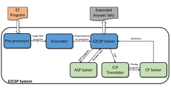
Figure 2: Architecture of the ezcsp system

Figure 2 depicts the architecture of the system, while the narrative below elaborates on the essential details. Both are focused on the functioning of the ezcsp system while employing the black-box integration schema.

The first step of the execution of ezcsp (corresponding to the Pre-processor component in the figure) consists in running a pre-processor, which translates an input ez program into a syntactically legal ASP program. This is accomplished by replacing the occurrences of arithmetic functions and operators in $required(\beta)$ atoms by auxiliary function symbols. For example, an atom $required(v\mathchar 62\relax 2)$ is replaced by $required(gt(v,2))$. A similar process is also applied to the notation for the specification of lists. For instance, an atom $required(all\_dif\!ferent([x,y]))$ is translated into $required(all\_dif\!ferent(list(x,y)))$. The Grounder component of the architecture transforms the resulting program into its propositional equivalent, a regular program, using an off-the-shelf grounder such as gringo (Gebser et al., 2007). This regular program is then passed to the ezcsp Solver component.

The ezcsp Solver component iterates ASP and constraint programming computations by invoking the corresponding components of the architecture. Specifically, the ASP Solver component computes an answer set of the regular program using an off-the-shelf ASP solver, such as cmodels or clasp. If an answer set is found, the ezcsp solver runs the CLP Translator component, which maps the csp-abstraction corresponding to the computed answer set to a Prolog program. The program is then passed to the CP Solver component, which uses the CLP solver embedded in a Prolog interpreter, e.g. SICStus or bprolog, to solve the CSP instance. For example, for the sample program presented in ${\mathit{E}xample}$ 5, the ezcsp system produces the answer set:

$$\{cspdomain(fd),cspvar(x,0,23),required(x\geq 12),switch,lightOn\}\mathbin{\cdot}$$

The csp-abstraction of the program with respect to this answer set is translated into a Prolog rule:

• $\displaystyle\hskip 25.00003pt{solve([x,V_{x}])\ :\mathchar 45\relax\ \ V_{x}\geq 0,\ \ V_{x}\leq 23,\ \ V_{x}\geq 12,\ \ labeling([V_{x}])\mathbin{\cdot}}$

In this case, the CLP solver embedded in the Prolog interpreter will find feasible assignments for variable $V_{x}$. The head of the rule is designed to return a complete solution and to ensure that the variable names used in the ez program are associated with the corresponding values. The interested reader can refer to Balduccini (2009a) for a complete description of the translation process.

Finally, the ezcsp Solver component gathers the solutions to the respective csp-abstraction and combines them with the answer set obtained earlier to form extended answer sets. Additional extended answer sets are computed iteratively by finding other answer sets and the solutions to the corresponding csp-abstractions.

5.2 Solving Algorithm

We are now ready to present our algorithm for computing answer sets of CA programs. In earlier work, Lierler (2014) demonstrated how the CASP language clingcon Gebser et al. (2009) as well as the essential subset of the CASP language AC of acsolver Mellarkod et al. (2008) are captured by CA programs. Based on those results, the algorithm described in this section can be immediately used as an alternative to the procedures implemented in systems clingcon and acsolver.

Usually, software systems are described by means of pseudocode. The fact that ezcsp system follows an “all-solvers-in-one” philosophy combined with a variety of integration schemas complicates the task of describing it in this way. For example, one configuration of ezcsp may invoke answer set solver clasp via black-box integration for enumerating answer sets of an asp-abstraction of CA program, whereas another may invoke cmodels via grey-box integration for the same task. Thus, rather than committing ourselves to a pseudocode description, we follow a path pioneered by Nieuwenhuis et al. (2006). In their work, the authors devised a graph-based abstract framework for describing backtrack search procedures for Satisfiability and SMT. Lierler (2014) designed a similar abstract framework that captures the ezcsp algorithm in two cases: (a) when ezcsp invokes answer set solver smodels via black-box integration for enumerating answer sets of asp-abstraction program, and (b) when ezcsp invokes answer set solver clasp via black-box integration.

In the present paper we introduce a graph-based abstract framework that is well suited for capturing the similarities and differences of the various configurations of ezcsp stemming from different integration schemas. The graph-based representation also allows us to speak of termination and correctness of procedures supporting these configurations. In this framework, nodes of a graph representing a solver capture its possible “states of computation”, while edges describe the possible transitions from one state to another. It should be noted that the graph representation is too high-level to capture some specific features of answer set solvers or constraint programming tools used within different ezcsp configurations. For example, the graph incorporates no information on the heuristic used to select a literal upon which a decision needs to be made. This is not an issue, however: stand alone answer set solvers have been analyzed and compared theoretically in the literature Anger et al. (2006), Giunchiglia et al. (2008) Lierler and Truszczyński (2011) as well as empirically in biennial answer set programming competitions Gebser et al. (2007), Denecker et al. (2009), Calimeri et al. (2011). At the same time, ezcsp treats constraint programming tools as “black-boxes” in all of its configurations.

5.2.1 Abstract ezcsp

Before introducing the transition system (graph) capable of capturing a variety of ezcsp procedures, we start by developing some required terminology. To make this section more self-contained we also restate some notation and definitions from earlier sections. Recall that for a set $M$ of literals, by $M^{\mathchar 43\relax}$ we denote the set of positive literals in $M$. For a CA program $\mathcal{P}\mathchar 61\relax\langle\Pi,\mathcal{C},\gamma,D\rangle$, a consistent and complete set $M$ of literals over $\mathit{At}(\Pi)$ is an answer set of $\mathcal{P}$ if

1. $M^{\mathchar 43\relax}$ is an answer set of $\Pi[\mathcal{C}]$ and

2. the constraint satisfaction problem $K_{\mathcal{P},M}$ has a solution.

As noted in Section 2.1 we can view denials as clauses. Given a denial $G$, by $G^{cl}$ we will denote a clause that corresponds to $G$, e.g., $(\leftarrow not\ pm)^{cl}$ denotes a clause $pm$. We may sometime abuse the notation and refer to a clause as if it were a denial. For instance, a clause $pm$ may denote a denial $\leftarrow not\ pm$.

We now introduce notions for CA programs that parallel ”entailment” for the case of classical logic formulas. Let $\mathcal{P}\mathchar 61\relax\langle\Pi,\mathcal{C},\gamma,D\rangle$ be a CA program. We say that $\mathcal{P}$ asp-entails a denial $G$ over $\mathit{At}(\Pi)$ when for every complete and consistent set $M$ of literals over $\mathit{At}(\Pi)$ such that $M^{\mathchar 43\relax}$ is an answer set of $\Pi[\mathcal{C}]$, $M$ satisfies $G^{cl}$. In other words, a denial is asp-entailed if any set of literals that satisfies the condition 1 of the answer set definition is such that it satisfies this denial. CA program $\mathcal{P}$ cp-entails a denial $G$ over $\mathit{At}(\Pi)$ when (i) for every answer set $M$ of $\mathcal{P}$, $M$ satisfies $G^{cl}$ and (ii) there is a complete and consistent set $N$ of literals over $\mathit{At}(\Pi)$ such that $N^{\mathchar 43\relax}$ is an answer set of $\Pi[\mathcal{C}]$ and $N$ does not satisfy $G$. Notice that if a denial $G$ is such that a CA program $\mathcal{P}$ cp-entails $G$, then $\mathcal{P}$ does not asp-entail $G$. We say that $\mathcal{P}$ entails a denial $G$ when $\mathcal{P}$ either asp-entails or cp-entails $G$. For a consistent set $N$ of literals over $\mathit{At}(\Pi)$ and a literal $l$, we say that $\mathcal{P}$ asp-entails $l$ with respect to $N$, if for every complete and consistent set $M$ of literals over $\mathit{At}(\Pi)$ such that $M^{\mathchar 43\relax}$ is an answer set of $\Pi[\mathcal{C}]$ and $N\subseteq M$, $l\in M$.

Example 8

Recall program $\mathcal{P}_{1}\mathchar 61\relax\langle\Pi_{1},\mathcal{C}_{1},\gamma_{1},D_{1}\rangle$ from ${\mathit{E}xample}$ 2. It is easy to check that denial $\leftarrow not\ lightOn\mathbin{\cdot}$ (or, in other words clause $lightOn$) is asp-entailed by $\mathcal{P}_{1}$. Also, $\mathcal{P}_{1}$ asp-entails literals $switch$ and $\neg am$ with respect to set $\{lightOn\}$ (and also with respect to $\emptyset$).

Let regular program $\Pi_{2}$ extend program $\Pi_{1}$ from ${\mathit{E}xample}$ 2 by rules

$$\begin{array}[]{l}\{pm\}\mathbin{\cdot}\\ \leftarrow\ not\ pm,\ |x\geq 12|\mathbin{\cdot}\\ \leftarrow\ |x\mathchar 60\relax 12|\mathbin{\cdot}\\ \end{array}$$

Consider a CA program $\mathcal{P}_{2}$ that differs from $\mathcal{P}_{1}$ only by substituting its first member $\Pi_{1}$ of quadruple $\langle\Pi_{1},\mathcal{C}_{1},\gamma_{1},D_{1}\rangle$ by $\Pi_{2}$. Denial $\leftarrow not\ pm$ (or clause $pm$) is cp-entailed by $\mathcal{P}_{2}$. Indeed, the only answer set of this program is $\{pm,\neg|x\mathchar 60\relax 12|,|x\geq 12|\}$. This set satisfies $(\leftarrow not\ pm)^{cl}$, in other words, clause $pm$. Consider set $\{\neg pm,\neg|x\mathchar 60\relax 12|,|x\geq 12|\}$ that does not satisfy clause $pm$. Set of atoms $\{\neg pm,\neg|x\mathchar 60\relax 12|,|x\geq 12|\}^{\mathchar 43\relax}\mathchar 61\relax\{|x\geq 12|\}$ is an answer set of $\Pi_{2}[\mathcal{C}_{1}]$.

For a CA program $\mathcal{P}\mathchar 61\relax\langle\Pi,\mathcal{C},\gamma,D\rangle$ and a set $\Gamma$ of denials, by $\mathcal{P}[\Gamma]$ we denote the CA program $\langle\Pi\cup\Gamma,\mathcal{C},\gamma,D\rangle$. The following propositions capture important properties underlying the introduced entailment notions.

Proposition 1

For a CA program $\mathcal{P}\mathchar 61\relax\langle\Pi,\mathcal{C},\gamma,D\rangle$ and a set $\Gamma$ of denials over $\mathit{At}(\Pi)$ if $\mathcal{P}$ asp-entails every denial in $\Gamma$ then (i) programs $\Pi[\mathcal{C}]$ and $(\Pi\cup\Gamma)[\mathcal{C}]$ have the same answer sets; (ii) CA programs $\mathcal{P}$ and $\mathcal{P}[\Gamma]$ have the same answer sets.

Proof 5.1.

We first show that condition (i) holds. From Theorem 1 and the fact that $\mathcal{P}$ asp-entails every denial in $\Gamma$ it follows that programs $\Pi[\mathcal{C}]$ and $(\Pi\cup\Gamma)[\mathcal{C}]$ have the same answer sets. Condition (ii) follows from (i) and the fact that $K_{\mathcal{P},M}\mathchar 61\relax K_{\mathcal{P}[\Gamma],M}$ for any answer set $M$ of $\Pi[\mathcal{C}]$ (and, consequently, for $(\Pi\cup\Gamma)[\mathcal{C}]$).

Proposition 5.2.

For a CA program $\mathcal{P}\mathchar 61\relax\langle\Pi,\mathcal{C},\gamma,D\rangle$ and a set $\Gamma$ of denials over $\mathit{At}(\Pi)$ if $\mathcal{P}$ cp-entails every denial in $\Gamma$ then CA programs $\mathcal{P}$ and $\mathcal{P}[\Gamma]$ have the same answer sets.

Proof 5.3.

Let $\mathcal{P}$ be a CA program $\langle\Pi,\mathcal{C},\gamma,D\rangle$. It is easy to see that (a) $\Pi[\mathcal{C}]\cup\Gamma\mathchar 61\relax(\Pi\cup\Gamma)[\mathcal{C}]$ and (b) $K_{\mathcal{P},M}\mathchar 61\relax K_{\mathcal{P}[\Gamma],M}$.

Right-to-left: Take $M$ to be an answer set of $\mathcal{P}$. By the definition of an answer set, (i) $M^{\mathchar 43\relax}$ is an answer set of $\Pi[\mathcal{C}]$ and (ii) the constraint satisfaction problem $K_{\mathcal{P},M}$ has a solution. Since $\mathcal{P}$ cp-entails every denial in $\Gamma$, we conclude that $M$ is a model of $\Gamma^{cl}$. By Theorem 1, $M^{\mathchar 43\relax}$ is an answer set of $\Pi[\mathcal{C}]\cup\Gamma$. From (a) and (b) we derive that $M$ is an answer set of $\mathcal{P}[\Gamma]$.

Left-to-right: Take $M$ to be an answer set of $\mathcal{P}[\Gamma]$. By the definition of an answer set, (i) $M^{\mathchar 43\relax}$ is an answer set of $(\Pi\cup\Gamma)[\mathcal{C}]$ and (ii) the constraint satisfaction problem $K_{\mathcal{P}[\Gamma],M}$ has a solution. From (i) and (a) it follows that $M^{\mathchar 43\relax}$ is an answer set of $\Pi[\mathcal{C}]\cup\Gamma$. By Theorem 1, $M^{\mathchar 43\relax}$ is an answer set of $\Pi[\mathcal{C}]$. By (b) and (ii) we derive that, $M$ is an answer set of $\mathcal{P}$.

Proposition 5.4.

For a CA program $\mathcal{P}\mathchar 61\relax\langle\Pi,\mathcal{C},\gamma,D\rangle$ and a set $\Gamma$ of denials over $\mathit{At}(\Pi)$ if $\mathcal{P}$ entails every denial in $\Gamma$ then (i) every answer set of $(\Pi\cup\Gamma)[\mathcal{C}]$ is also an answer set of $\Pi[\mathcal{C}]$; (ii) CA programs $\mathcal{P}$ and $\mathcal{P}[\Gamma]$ have the same answer sets.

Proof 5.5.

Condition (i) follows from Theorem 1 and the fact that $(\Pi)[\mathcal{C}]$ and $(\Pi\cup\Gamma)[\mathcal{C}]$ only differ in denials.

We now show that condition (ii) holds. Set $\Gamma$ is composed of two disjoint sets $\Gamma_{1}$ and $\Gamma_{2}$ (i.e., $\Gamma\mathchar 61\relax\Gamma_{1}\cup\Gamma_{2}$), where $\Gamma_{1}$ is the set of all denials that are asp-entailed by $\mathcal{P}$ and $\Gamma_{2}$ is the set of all denials that are cp-entailed by $\mathcal{P}$. By Proposition 1 (ii), CA programs $\mathcal{P}$ and $\mathcal{P}[\Gamma_{1}]$ have the same answer sets. By Proposition 5.2, CA programs $\mathcal{P}[\Gamma_{1}]$ and $\mathcal{P}[\Gamma_{1}\cup\Gamma_{2}]$ have the same answer sets. It immediately follows that CA programs $\mathcal{P}$ and $\mathcal{P}[\Gamma_{1}\cup\Gamma_{2}]$ have the same answer sets.

For an alphabet $\sigma$, a record relative to $\sigma$ is a sequence $M$ composed of distinct literals over $\sigma$ or symbol $\bot$, some literals are possibly annotated by the symbol $\Delta$, which marks them as decision literals such that:

1. the set of literals in $M$ is consistent or $M\mathchar 61\relax M^{\prime}l$, where the set of literals in $M^{\prime}$ is consistent and contains $\overline{l}$,

2. if $M\mathchar 61\relax M^{\prime}l^{\Delta}M^{\prime\prime}$, then neither $l$ nor its dual $\overline{l}$ is in $M^{\prime}$, and

3. if $\bot$ occurs in $M$, then $M\mathchar 61\relax M^{\prime}\bot$ and $M^{\prime}$ does not contain $\bot$.

We often identify records with the set of its members disregarding annotations.

For a CA program $\mathcal{P}\mathchar 61\relax\langle\Pi,\mathcal{C},\gamma,D\rangle$, a state relative to $\mathcal{P}$ is either a distinguished state Failstate or a triple $M||\Gamma||\Lambda$ where $M$ is a record relative to $\mathit{At}(\Pi)$; $\Gamma$ and $\Lambda$ are each a set of denials that are entailed by $\mathcal{P}$. Given a state $M||\Gamma||\Lambda$ if neither a literal $l$ nor $\overline{l}$ occurs in $M$, then $l$ is unassigned by the state; if  $\bot$ does not occur in $M$ as well as for any atom $a$ it is not the case that both $a$ and $\neg a$ occur in $M$, then this state is consistent. For a state $M||\Gamma||\Lambda$, we call $M$, $\Gamma$, and $\Lambda$ the atomic, permanent, and temporal parts of the state, respectively. The role of the atomic part of the state is to track decisions (choices) as well as inferences that the solver has made. The permanent and temporal parts are responsible for assisting the solver in accumulating additional information – entailed denials by a given program – that becomes apparent during the search process.

$\begin{array}[t]{lll}\hbox{{\hbox{{Decide}}}:}&M||\Gamma||\Lambda\leavevmode\nobreak\ \Rightarrow\leavevmode\nobreak\ M\leavevmode\nobreak\ l^{\Delta}||\Gamma||\Lambda&\hbox{if $l$ is unassigned by $M$ and $M$ is consistent}\\ \\ \hbox{{\hbox{{Fail}}}:}&M||\Gamma||\Lambda\leavevmode\nobreak\ \Rightarrow\leavevmode\nobreak\ {\hbox{{Failstate}}}&\hbox{if \leavevmode\nobreak\ }\left\{\begin{array}[]{l}\hbox{$M$ is inconsistent and}\\ \hbox{$M$ contains no decision literals}\\ \end{array}\right\mathbin{\cdot}\\ \\ \hbox{{\hbox{{Backtrack}}}:}&P\leavevmode\nobreak\ l^{\Delta}\leavevmode\nobreak\ Q||\Gamma||\Lambda\Rightarrow\leavevmode\nobreak\ P\leavevmode\nobreak\ \overline{l}||\Gamma||\Lambda&\hbox{if \leavevmode\nobreak\ }\left\{\begin{array}[]{l}\hbox{$P\leavevmode\nobreak\ l^{\Delta}\leavevmode\nobreak\ Q$ is inconsistent, and}\\ \hbox{$Q$ contains no decision literals.}\end{array}\right\mathbin{\cdot}\\ \\ \hbox{{\hbox{{ASP-Propagate}}}:}&M||\Gamma||\Lambda\leavevmode\nobreak\ \Rightarrow\leavevmode\nobreak\ M\leavevmode\nobreak\ l||\Gamma||\Lambda&\hbox{if \leavevmode\nobreak\ }\hbox{$\mathcal{P}[\Gamma\cup\Lambda]$ asp-entails $l$ with respect to $M$}\\ \\ \hbox{{\hbox{{CP-Propagate}}}:}&M||\Gamma||\Lambda\leavevmode\nobreak\ \Rightarrow\leavevmode\nobreak\ M\leavevmode\nobreak\ \bot||\Gamma||\Lambda&\hbox{if $K_{\mathcal{P},M}$ has no solution}\\ \\ \hbox{{\hbox{{Learn}}}:}&M||\Gamma||\Lambda\leavevmode\nobreak\ \Rightarrow\leavevmode\nobreak\ M||\Gamma\cup\{R\}||\Lambda&\hbox{if }\mathcal{P}[\Gamma\cup\Lambda]\hbox{ entails denial $R$ {\color[rgb]{0,0,0}and $R\not\in\Gamma\cup\Lambda$ }}\\ \\ \hbox{{\hbox{{Learn${}^{t}$}}}:}&M||\Gamma||\Lambda\leavevmode\nobreak\ \Rightarrow\leavevmode\nobreak\ M||\Gamma||\Lambda\cup\{R\}&\hbox{if }\mathcal{P}[\Gamma\cup\Lambda]\hbox{ entails denial $R$ {\color[rgb]{0,0,0}and $R\not\in\Gamma\cup\Lambda$} }\\ \\ \hbox{{\hbox{{Restart}}}:}&M||\Gamma||\Lambda\leavevmode\nobreak\ \Rightarrow\leavevmode\nobreak\ \emptyset||\Gamma||\Lambda&\hbox{if }M\neq\emptyset\\ \\ \hbox{{\hbox{{Restart${}^{t}$}}}:}&M||\Gamma||\Lambda\leavevmode\nobreak\ \Rightarrow\leavevmode\nobreak\ \emptyset||\Gamma||\emptyset&\hbox{if }M\neq\emptyset\\ \\ \end{array}$

Figure 3: The transition rules of the graph $\hbox{{ez}}_{\mathcal{P}}$.

$\begin{array}[]{lc}\emptyset||\emptyset||\emptyset&\stackrel{{\scriptstyle\hbox{{ASP-Propagate}}}}{{\Rightarrow}}\\ \\ lightOn||\emptyset||\emptyset&\stackrel{{\scriptstyle\hbox{{ASP-Propagate}}}}{{\Rightarrow}}\\ \\ lightOn\ switch||\emptyset||\emptyset&\stackrel{{\scriptstyle\hbox{{ASP-Propagate}}}}{{\Rightarrow}}\\ \\ lightOn\ switch\ \neg am||\emptyset||\emptyset&\stackrel{{\scriptstyle\hbox{{ASP-Propagate}}}}{{\Rightarrow}}\\ \\ lightOn\ switch\ \neg am\ \neg|x\mathchar 60\relax 12|\leavevmode\nobreak\ ||\emptyset||\emptyset&\stackrel{{\scriptstyle\hbox{{Decide}}}}{{\Rightarrow}}\\ \\ lightOn\ switch\ \neg am\ \neg|x\mathchar 60\relax 12|\ \neg|x\geq 12|^{\Delta}||\emptyset||\emptyset&\stackrel{{\scriptstyle\hbox{{CP-Propagate}}}}{{\Rightarrow}}\\ \\ lightOn\ switch\ \neg am\ \neg|x\mathchar 60\relax 12|\ \neg|x\geq 12|^{\Delta}\ \bot||\emptyset||\emptyset&\stackrel{{\scriptstyle\hbox{{Backtrack}}}}{{\Rightarrow}}\\ \\[7.22743pt] lightOn\ switch\ \neg am\ \neg|x\mathchar 60\relax 12|\ |x\geq 12|\ ||\emptyset||\emptyset&\end{array}$

Figure 4: Sample path in graph ${\textsc{ez}}_{\mathcal{P}_{1}}$.

We now define a graph ez_P for a CA program $\mathcal{P}$. Its nodes are the states relative to $\mathcal{P}$. These nodes intuitively correspond to states of computation. The edges of the graph ez_P are specified by nine transition rules presented in Figure 3. These rules correspond to possible operations by the ezcsp system that bring it from one state of computation to another. A path in the graph $\hbox{{ez}}_{\mathcal{P}}$ is a description of a process of search for an answer set of $\mathcal{P}$. The process is captured via applications of transition rules. Theorem 3 introduced later in this section makes this statement precise.

Example 5.6.

Recall CA program $\mathcal{P}_{1}\mathchar 61\relax\langle\Pi_{1},\mathcal{C}_{1},\gamma_{1},D_{1}\rangle$ introduced in ${\mathit{E}xample}$ 2. Figure 4 presents a sample path in ${\textsc{ez}}_{\mathcal{P}_{1}}$ with every edge annotated by the name of a transition rule that justifies the presence of this edge in the graph.

Now we turn our attention to an informal discussion of the role of each of the transition rules in $\hbox{{ez}}_{\mathcal{P}}$.

5.2.2 Informal account on transition rules

We refer to the transition rules Decide, Fail, Backtrack, ASP-Propagate, CP-Propagate of the graph $\hbox{{ez}}_{\mathcal{P}}$ as basic.

The unique feature of basic rules is that they only concern the atomic part of a state. Consider a state $S\mathchar 61\relax M||\Gamma||\Lambda$. An application of any basic rule results in a state whose permanent and temporal parts remain unchanged, i.e., $\Gamma$ and $\Lambda$ respectively (unless it is the case of Fail).

Decide

An application of the transition rule Decide to $S$ results in a state whose atomic part has the form $M\leavevmode\nobreak\ l^{\Delta}$. Intuitively this rule allows us to pursue evaluation of assignments that assume value of literal $l$ to be true. The fact that this literal is marked by $\Delta$ suggests that we can still reevaluate this assumption in the future, in other words to backtrack on this decision.

Fail

The transition rule Fail specifies the conditions on atomic part $M$ of state $S$ suggesting that Failstate is reachable from $M$. Intuitively, if our computation brought us to such a state transition to Failstate confirms that there is no solution to the problem.

Backtrack

The transition rule Backtrack specifies the conditions on atomic part of the state suggesting when it is time to backtrack and what the new atomic part of the state is after backtracking. Rules Fail and Backtrack share one property: they are applicable only when states are inconsistent.

ASP-Propagate

The transition rule ASP-Propagate specifies the condition under which a new literal $l$ (without a decision annotation) is added to an atomic part. Such rules are commonly called propagators. Note that the condition of ASP-Propagate

$$\mathcal{P}[\Gamma\cup\Lambda] l M$$ asp-entails with respect to (14)

is defined over a program extended by permanent and temporal part. This fact illustrates the role of these entities. They carry extra information aquired/learnt during the computation. Also condition (14) is semantic. It refers to the notion of asp-entailment, which is defined by a reference to the semantics of a program. Propagators used by software systems typically use syntactic conditions, which are easy to check by inspecting syntactic properties of a program. Later in this section we present instances of such propagators, in particular, propagators that are used within the ezcsp solver.

CP-Propagate

The transition rule CP-Propagate specifies the condition under which symbol $\bot$ is added to an atomic part. Thus it leads to a state that is inconsistent suggesting that the search process is either ready to fail or to backtrack. The condition of CP-Propagate

$$K_{\mathcal{P},M}$$ has no solution

represents a decision procedure that establishes whether the CSP problem $K_{\mathcal{P},M}$ has solutions or not.

We now turn our attention to non-basic rules that concern permanent and temporal parts of the states of computation.

Learn

Recall the definition of the transition rule Learn

• $\displaystyle\hskip 25.00003pt{M||\Gamma||\Lambda\leavevmode\nobreak\ \Rightarrow\leavevmode\nobreak\ M||\Gamma\cup\{R\}||\Lambda\hbox{ \leavevmode\nobreak\ \leavevmode\nobreak\ if\leavevmode\nobreak\ \leavevmode\nobreak\ }\mathcal{P}[\Gamma\cup\Lambda]\hbox{ entails denial $R$ {\color[rgb]{0,0,0}and $R\not\in\Gamma\cup\Lambda$ }}}$

An application of this rule to a state $M||\Gamma||\Lambda$, results in a state whose atomic and temporal parts stay unchanged. The permanent part is extended by a denial $R$. Intuitively the effect of this rule is such that from this point of computation the “permanent” denial becomes effectively a part of the program being solved. This is essential for two reasons. First, if the learnt denial $R$ is cp-entailed then $\Pi\cup\Gamma\cup\Lambda$ and $\Pi\cup\Gamma\cup\Lambda\cup\{R\}$ are programs with different answer sets. In turn, the rule ASP-Propagate may be applicable to some state $N||\Gamma\cup\{R\}||\Lambda$ and not to $N||\Gamma||\Lambda$. Similarly, due to the fact that only “syntactic” instances of ASP-Propagate are implemented in solvers, the previous statement also holds for the case when $R$ is asp-entailed.

Learn^t

The role of the transition rule Learn^t is similar to that of Learn, but the learnt denials by this rule are not meant to be preserved permanently in the computation.

Restart and Restart^t

The transition rule Restart allows the computation to start from “scratch” with respect to atomic part of the state. The transition rule Restart^t forces the computation to start from “scratch” with respect to not only atomic part of the state but also all temporally learnt denials. These restart rules are essential in understanding the key differences between various integration strategies that are of focus in this paper.

5.2.3 Formal properties of ${\hbox{{ez}}}_{\mathcal{P}}$

We call the state $\emptyset||\emptyset||\emptyset$ — initial. We say that a node in the graph is semi-terminal if no rule other than Learn, Learn^t, Restart, Restart^t is applicable to it (or, in other words, if no single basic rule is applicable to it). We say that a path in ${\hbox{{ez}}}_{\mathcal{P}}$ is restart-safe when, prior to any edge $e$ due to an application of Restart or Restart^t on this path, there is an edge $e^{\prime}$ due to an application of Learn such that: (i) edge $e^{\prime}$ precedes $e$; (ii) $e^{\prime}$ does not precede any other edge $e^{\prime\prime}\neq e$ due to Restart or Restart^t. We say that a restart-safe path $t$ is maximal if (i) the first state in $t$ is an initial state, and (ii) $t$ is not a subpath of any restart-safe path $t^{\prime}\neq t$.

Example 5.7.

Recall CA program $\mathcal{P}_{1}\mathchar 61\relax\langle\Pi_{1},\mathcal{C}_{1},\gamma_{1},D_{1}\rangle$ introduced in ${\mathit{E}xample}$ 2. Trivially a sample path in ${\textsc{ez}}_{\mathcal{P}_{1}}$ in Figure 4 is a restart-safe path. A nontrivial example of restart-safe path in ${\textsc{ez}}_{\mathcal{P}_{1}}$ follows

$$\begin{array}[]{lc}\emptyset||\emptyset||\emptyset&\stackrel{{\scriptstyle\hbox{{Learn}}}}{{\Rightarrow}}\\ \\ \emptyset||\{\leftarrow not\ switch\}||\emptyset&\stackrel{{\scriptstyle\hbox{{ASP-Propagate}}}}{{\Rightarrow}}\\ \\ lightOn||\{\leftarrow not\ switch\}||\emptyset&\stackrel{{\scriptstyle\hbox{{Restart}}}}{{\Rightarrow}}\\ \\ \emptyset||\{\leftarrow not\ switch\}||\emptyset\mathbin{\cdot}&\end{array}$$ (15)

Similarly, a path that extends the path above as follows

$$\begin{array}[]{lc}&\stackrel{{\scriptstyle\hbox{{Learn}}}}{{\Rightarrow}}\\ \\ \emptyset||\{\leftarrow not\ switch,\ \leftarrow am\}||\emptyset&\stackrel{{\scriptstyle\hbox{{ASP-Propagate}}}}{{\Rightarrow}}\\ \\ lightOn||\{\leftarrow not\ switch,\ \leftarrow am\}||\emptyset&\stackrel{{\scriptstyle\hbox{{Restart}}}}{{\Rightarrow}}\\ \\ \emptyset||\{\leftarrow not\ switch,\ \leftarrow am\}||\emptyset&\end{array}$$

is restart-safe.

A simple path in ${\textsc{ez}}_{\mathcal{P}_{1}}$ that is not restart-safe

• $\displaystyle\hskip 25.00003pt{\begin{array}[]{lc}\emptyset||\emptyset||\emptyset&\stackrel{{\scriptstyle\hbox{{ASP-Propagate}}}}{{\Rightarrow}}\\ lightOn||\emptyset||\emptyset&\stackrel{{\scriptstyle\hbox{{Restart}}}}{{\Rightarrow}}\\ \emptyset||\emptyset||\emptyset\mathbin{\cdot}&\end{array}}$

Indeed, condition (i) of the restart-safe definition does not hold. Another example of a not restart-safe path is a path that extends path (15) as follows

$$\begin{array}[]{lc}&\stackrel{{\scriptstyle\hbox{{ASP-Propagate}}}}{{\Rightarrow}}\\ \\ lightOn||\{\leftarrow not\ switch\}||\emptyset&\stackrel{{\scriptstyle\hbox{{Restart}}}}{{\Rightarrow}}\\ \\ \emptyset||\{\leftarrow not\ switch\}||\emptyset\mathbin{\cdot}&\end{array}$$

Indeed, condition (ii) of the restart-safe definition does not hold for the second occurrence of the Restart edge.

The following theorem captures key properties of the graph ${\hbox{{ez}}}_{\mathcal{P}}$. They suggest that the graph can be used for deciding whether a program with constraint atoms has an answer set.

Theorem 3.

For any CA program $\mathcal{P}$:

• every restart-safe path in $\hbox{{ez}}_{\mathcal{P}}$ is finite, and any maximal restart-safe path ends with a state that is semi-terminal,

• for any semi-terminal state $M||\Gamma||\Lambda$ of $\hbox{{ez}}_{\mathcal{P}}$ reachable from initial state, $M$ is an answer set of $\mathcal{P}$,

• state Failstate is reachable from initial state in $\hbox{{ez}}_{\mathcal{P}}$ by a restart-safe path if and only if $\mathcal{P}$ has no answer set.

On the one hand, part (a) of Theorem 3 asserts that, if we construct a restart-safe path from initial state, then some semi-terminal state is eventually reached. On the other hand, parts (b) and (c) assert that, as soon as a semi-terminal state is reached by following any restart-safe path, the problem of deciding whether CA program $\mathcal{P}$ has answer sets is solved. Section 5.3 describes the varying configurations of the ezcsp system.

Example 5.8.

Recall ${\mathit{E}xample}$ 5.6. Since the last state in the sample path presented in Figure (4) is semi-terminal, Theorem 3 asserts that the set of literals composed of the elements of this semi-terminal state forms the answer set of CA program $\mathcal{P}_{1}$. Indeed, this set coincides with the answer set $M_{1}$ of $\mathcal{P}_{1}$ presented in ${\mathit{E}xample}$ 3.

In our discussion of the transition rule ASP-Propagate we mentioned how the ezcsp solver accounts only for some transitions due to this rule. Let $\mathcal{P}\mathchar 61\relax\langle\Pi,\mathcal{C},\gamma,D\rangle$ be a CA program. By $\hbox{{ezsm}}_{\mathcal{P}}$ we denote an edge-induced subgraph of $\hbox{{ez}}_{\mathcal{P}}$, where we drop the edges that correspond to the application of transition rules ASP-Propagate not accounted by the following two transition rules (propagators) Unit Propagate and Unfounded:

• $\displaystyle\hskip 25.00003pt{\begin{array}[t]{l}\hbox{{\hbox{{Unit Propagate}}}: }M||\Gamma||\Lambda\leavevmode\nobreak\ \Rightarrow\leavevmode\nobreak\ M\leavevmode\nobreak\ l||\Gamma||\Lambda\left\{\begin{array}[]{l}\hbox{$C\vee l\in{(\Pi[\mathcal{C}]\cup\Gamma\cup\Lambda)^{cl}}$,}\\ \hbox{$M$ is consistent,}\\ \hbox{$M\models\overline{C}$}\\ \end{array}\right\mathbin{\cdot}\\ \\ \hbox{{\hbox{{Unfounded}}}: }M||\Gamma||\Lambda\leavevmode\nobreak\ \Rightarrow\leavevmode\nobreak\ M\leavevmode\nobreak\ l||\Gamma||\Lambda\left\{\begin{array}[]{l}\hbox{$M$ is consistent, and there is literal $l$ so that}\\ \hbox{$\overline{l}\in U$ for a set $U$, which is}\\ \hbox{unfounded on $M$ w.r.t. $\Pi[\mathcal{C}]\cup\Gamma\cup\Lambda$}\\ \end{array}\right\mathbin{\cdot}\\ \\ \end{array}}$

These two propagators rely on properties that can be checked by efficient procedures. The conditions of these transition rules are such that they are satisfied only if $\mathcal{P}[\Gamma\cup\Lambda]$ asp-entails $l$ w.r.t. $M$. In other words, the transition rules Unit Propagate or Unfounded are applicable only in states where ASP-Propagate is applicable. The other direction is not true. Theorem 3 holds if we replace $\hbox{{ez}}_{\mathcal{P}}$ by $\hbox{{ezsm}}_{\mathcal{P}}$ in its statement. The proof of this theorem relies on the statement of Theorem 2, and is given at the end of this subsection. Graph $\hbox{{ezsm}}_{\mathcal{P}}$ is only one of the possible subgraphs of the generic graph $\hbox{{ez}}_{\mathcal{P}}$ that share its key properties stated in Theorem 3. These properties show that graph $\hbox{{ezsm}}_{\mathcal{P}}$ gives rise to a class of correct algorithms for computing answer sets of programs with constraints. It provides a proof of correctness of every CASP solver in this class and a proof of termination under the assumption that restart-safe paths are considered by a solver. Note how much weaker propagators, such as Unit Propagate and Unfounded, than ASP-Propagate are sufficient to ensure the correctness of respective solving procedures. We picked the graph $\hbox{{ezsm}}_{\mathcal{P}}$ for illustration as it captures the essential propagators present in modern (constraint) answer set solvers and allows a more concrete view on the $\hbox{{ez}}_{\mathcal{P}}$ framework. Yet the goal of this work is not to detail the variety of possible propagators of (constraint) answer set solvers but master the understanding of hybrid procedures that include this technology. Therefore in the rest of this section we turn our attention back to the $\hbox{{ez}}_{\mathcal{P}}$ graph and use this graph to formulate black-box, grey-box, and clear-box configurations of the CASP solver ezcsp.

The rest of this subsection presents a proof of Theorem 3 as well as a proof of the similar theorem for the graph $\hbox{{ezsm}}_{\mathcal{P}}$.

Proof 5.9 (Proof of Theorem 3).

(a) Let $\mathcal{P}$ be a CA program $\langle\Pi,\mathcal{C},\gamma,D\rangle$.

We first show that any path in $\hbox{{ez}}_{\mathcal{P}}$ that does not contain Restart^t or Restart edges is finite. We name this statement Statement 1.

Consider any path $t$ in $\hbox{{ez}}_{\mathcal{P}}$ that does not contain Restart^t or Restart edges.

For any list $N$ of literals, by $|N|$ we denote the length of $N$. Any state $M||\Gamma||\Lambda$ has the form $M_{0}\leavevmode\nobreak\ l^{\Delta}_{1}\leavevmode\nobreak\ M_{1}\dots l^{\Delta}_{p}\leavevmode\nobreak\ M_{p}||\Gamma||\Lambda$, where $l^{\Delta}_{1}\dots l^{\Delta}_{p}$ are all decision literals of $M$; we define $\alpha(M||\Gamma||\Lambda)$ as the sequence of nonnegative integers $|M_{0}|,|M_{1}|,\dots,|M_{p}|$, and $\alpha(\hbox{{Failstate}})\mathchar 61\relax\infty$. For any two states, $S$ and $S^{\prime}$, of ${\hbox{{ez}}}_{\mathcal{P}}$, we understand $\alpha(S)\mathchar 60\relax\alpha(S^{\prime})$ as the lexicographical order. We note that, for any state $M||\Gamma||\Lambda$, the value of $\alpha$ is based only on the first component, $M$, of the state. Second, there is a finite number of distinct values of $\alpha$ for the states of ${\hbox{{ez}}}_{\mathcal{P}}$ due to the fact that there is a finite number of distinct $M$’s over $\mathcal{P}$. We now define relation smaller over the states of ${\hbox{{ez}}}_{\mathcal{P}}$. We say that state $M||\Gamma||\Lambda$ is smaller than state $M^{\prime}||\Gamma^{\prime}||\Lambda^{\prime}$ when either

1. $\Gamma\subset\Gamma^{\prime}$, or

2. $\Gamma\mathchar 61\relax\Gamma^{\prime}$, and $\Lambda\subset\Lambda^{\prime}$, or

3. $\Gamma\mathchar 61\relax\Gamma^{\prime}$, $\Lambda\mathchar 61\relax\Lambda^{\prime}$, and $\alpha(M||\Gamma||\Lambda)\mathchar 60\relax\alpha(M^{\prime}||\Gamma^{\prime}||\Lambda^{\prime})$.

It is easy to see that this relation is anti-symmetric and transitive.

By the definition of the transition rules of ${\hbox{{ez}}}_{\mathcal{P}}$, if there is an edge from $M||\Gamma||\Lambda$ to $M^{\prime}||\Gamma^{\prime}||\Lambda^{\prime}$ in ${\hbox{{ez}}}_{\mathcal{P}}$ formed by any basic transition rule or rules Learn or Learn^t, then $M||\Gamma||\Lambda$ is smaller than state $M^{\prime}||\Gamma^{\prime}||\Lambda^{\prime}$. Observe that (i) there is a finite number of distinct values of $\alpha$, and (ii) there is a finite number of distinct denials entailed by $\mathcal{P}$. Then, it follows that there is only a finite number of edges in $t$, and, thus, Statement 1 holds.

We call a subpath from state $S$ to state $S^{\prime}$ of some path in $\hbox{{ez}}_{\mathcal{P}}$ restarting when (i) an edge that follows $S$ is due to the application of rule Learn, (ii) an edge leading to $S^{\prime}$ is due to the application of rule Restart^t or Restart, and (iii) on this subpath, there are no other edges due to applications of Learn, Restart^t, or Restart, but the ones mentioned above. Using Statement 1, it follows that any restarting subpath is finite.

Consider any restart-safe path $r$ in $\hbox{{ez}}_{\mathcal{P}}$. We construct a path $r^{\prime}$ by dropping some finite fragments from $r$. This is accomplished by replacing each restarting subpath of $r$ from state $S$ to state $S^{\prime}$ by an edge from $S$ to $S^{\prime}$ that we call Artificial. It is easy to see that an edge in $r^{\prime}$ due to Artificial leads from a state of the form $M||\Gamma||\Lambda$ to a state $\emptyset||\Gamma\cup\{C\}||\Lambda^{\prime}$, where $C$ is a denial. Indeed, within a restarting subpath an edge due to rule Learn occurred introducing denial $C$. State $M||\Gamma||\Lambda$ is smaller than the state $\emptyset||\Gamma\cup\{C\}||\Lambda^{\prime}$. At the same time, $r^{\prime}$ contains no edges due to applications of Restart^t or Restart. Indeed, we eliminated these edges in favor of edges called Artificial. Thus by the same argument as in the proof of Statement 1, $r^{\prime}$ contains a finite number of edges. We can now conclude that $r$ is finite.

It is easy to see that maximal restart-safe path ends with a state that is semi-terminal. Indeed, assume the opposite: there is a maximal restart-safe path $t$, which ends in a non semi-terminal state $S$. Then, some basic rule applies to state $S$. Consider path $t^{\prime}$ consisting of path $t$ and a transition due to a basic rule applicable to $S$. Note that $t^{\prime}$ is also a restart-safe path, and that $t$ is a subpath of $t^{\prime}$. This contradicts the definition of maximal.

(b) Let $M||\Gamma||\Lambda$ be a semi-terminal state so that none of the Basic rules are applicable. From the fact that Decide is not applicable, we conclude that $M$ assigns all literals or $M$ is inconsistent.

We now show that $M$ is consistent. Proof by contradiction. Assume that $M$ is inconsistent. Then, since Fail is not applicable, $M$ contains a decision literal. Consequently, $M||\Gamma||\Lambda$ is a state in which Backtrack is applicable. This contradicts our assumption that $M||\Gamma||\Lambda$ is semi-terminal.

Also, $M^{\mathchar 43\relax}$ is an answer set of $\Pi[\mathcal{C}]$. Proof by contradiction. Assume that $M^{\mathchar 43\relax}$ is not an answer set of $\Pi[\mathcal{C}]$. It follows that that $M$ is not an answer set of $\mathcal{P}$. By Proposition 5.4, it follows that $M$ is not an answer set of $\mathcal{P}[\Gamma\cup\Lambda]$ and $M^{\mathchar 43\relax}$ is not an answer of $\Pi[\mathcal{C}]\cup\Gamma\cup\Lambda$. Recall that $\mathcal{P}[\Gamma\cup\Lambda]$ asp-entails a literal $l$ with respect to $M$ if for every complete and consistent set $M^{\prime}$ of literals over $\mathit{At}(\Pi)$ such that $M^{\prime\mathchar 43\relax}$ is an answer set of $\Pi[\mathcal{C}]\cup\Gamma\cup\Lambda$ and $M\subseteq M^{\prime}$, $l\in M^{\prime}$. Since $M$ is complete and consistent set of literals over $\mathit{At}(\Pi)$ it follows that there is no complete and consistent set $M^{\prime}$ of literals over $\mathit{At}(\Pi)$ such that $M\subseteq M^{\prime}$ and $M^{\prime\mathchar 43\relax}$ is an answer set of $\Pi[\mathcal{C}]\cup\Gamma\cup\Lambda$. We conclude that $\mathcal{P}[\Gamma\cup\Lambda]$ asp-entails any literal $l$. Take $l$ to be a complement of some literal occurring in $M$. It follows that ASP-Propagate is applicable in state $M||\Gamma||\Lambda$ allowing a transition to state $M\leavevmode\nobreak\ l||\Gamma||\Lambda$. This contradicts our assumption that $M||\Gamma||\Lambda$ is semi-terminal.

CSP $K_{\mathcal{P},M}$ has a solution. This immediately follows from the application condition of the transition rule CP-Propagate and the fact that the state $M||\Gamma||\Lambda$ is semi-terminal.

From the conclusions that $M^{\mathchar 43\relax}$ is an answer set of $\Pi[\mathcal{C}]$ and $K_{\mathcal{P},M}$ has a solution we derive that $M$ is an answer set of $\mathcal{P}$.

(c) We start by proving an auxiliary statement:

Statement 2: For any CA program $\mathcal{P}$, and a path from an initial state to $l_{1}\dots l_{n}||\Gamma||\Lambda$ in $\hbox{{ez}}_{\mathcal{P}}$, every answer set $X$ for $\mathcal{P}$ satisfies $l_{i}$ if it satisfies all decision literals $l_{j}^{\Delta}$ with $j\leq i$.

By induction on the length of a path. Since the property trivially holds in the initial state, we only need to prove that all transition rules of $\hbox{{ez}}_{\mathcal{P}}$ preserve it.

Consider an edge $M||\Gamma||\Lambda\Rightarrow S$ where $S$ is either a fail state or state of the form $M^{\prime}||\Gamma^{\prime}||\Lambda^{\prime}$, $M$ is a sequence $l_{1}\leavevmode\nobreak\ \dots\leavevmode\nobreak\ l_{k}$ such that every answer set $X$ of $\mathcal{P}$ satisfies $l_{i}$ if it satisfies all decision literals $l^{\Delta}_{j}$ with $j\leq i$.

Decide, Fail, CP-Propagate Learn, Learn^t, Restart, Restart^t: Obvious.

ASP-Propagate: $M^{\prime}||\Gamma^{\prime}||\Lambda^{\prime}$ is $M\leavevmode\nobreak\ l_{k\mathchar 43\relax 1}||\Gamma||\Lambda$. Take any answer set $X$ of $\mathcal{P}$ such that $X$ satisfies all decision literals $l^{\Delta}_{j}$ with $j\leq k\mathchar 43\relax 1$. From the inductive hypothesis it follows that $X$ satisfies $M$. Consequently, $M\subseteq X$ since $X$ is a consistent and complete set of literals. From the definition of ASP-Propagate, $\mathcal{P}$ asp-entails $l_{k\mathchar 43\relax 1}$ with respect to $M$. We also know that $X^{\mathchar 43\relax}$ is an answer set of $\Pi[\mathcal{C}]$. Thus, $l_{k\mathchar 43\relax 1}\in X$.

Backtrack: $M$ has the form $P\leavevmode\nobreak\ l^{\Delta}_{i}\leavevmode\nobreak\ Q$ where $Q$ contains no decision literals. $M^{\prime}||\Gamma^{\prime}||\Lambda^{\prime}$ has the form $P\leavevmode\nobreak\ \overline{l_{i}}||\Gamma||\Lambda$. Take any answer set $X$ of $\mathcal{P}$ such that $X$ satisfies all decision literals $l^{\Delta}_{j}$ with $j\leq i$. We need to show that $X\models\overline{l_{i}}$. By contradiction. Assume that $X\models\leavevmode\nobreak\ \!\!{l_{i}}$. By the inductive hypothesis, since $Q$ does not contain decision literals, it follows that $X$ satisfies $P\leavevmode\nobreak\ l^{\Delta}_{i}\leavevmode\nobreak\ Q$, that is, $M$. This is impossible because $M$ is inconsistent. Hence, $X\models\overline{l_{i}}$.

Left-to-right: Since Failstate is reachable from the initial state by a restart-safe path, there is an inconsistent state $M||\Gamma||\Lambda$ without decision literals such that there exists a path from the initial state to $M||\Gamma||\Lambda$. By Statement 2, any answer set of $\mathcal{P}$ satisfies $M$. Since $M$ is inconsistent we conclude that $\mathcal{P}$ has no answer sets.

Right-to-left: From (a) it follows that any maximal restart-safe path is a path from initial state to some semi-terminal state $S$. By (b), this state $S$ cannot be different from Failstate, because $\mathcal{P}$ has no answer sets.

Theorem 4.

For any CA program $\mathcal{P}$,

• every restart-safe path in $\hbox{{ezsm}}_{\mathcal{P}}$ is finite, and any maximal restart-safe path ends with a state that is semi-terminal,

• for any semi-terminal state $M||\Gamma||\Lambda$ of $\hbox{{ezsm}}_{\mathcal{P}}$ reachable from initial state, $M$ is an answer set of $\mathcal{P}$,

• state Failstate is reachable from initial state in $\hbox{{ezsm}}_{\mathcal{P}}$ by a restart-safe path if and only if $\mathcal{P}$ has no answer sets.

Proof 5.10.

Let $\mathcal{P}$ be a CA program $\langle\Pi,\mathcal{C},\gamma,D\rangle$.

(a) This part is proved as part (a) in proof of Theorem 3.

(b) Let $M||\Gamma||\Lambda$ be a semi-terminal state so that none of the basic rules are applicable (Unit Propagate and Unfounded are basic rules). As in proof of part (b) in Theorem 3 we conclude that $M$ assigns all literals and is consistent. Also, CSP $K_{\mathcal{P},M}$ has a solution.

We now illustrate that, $M^{\mathchar 43\relax}$ is an answer set of $\Pi[\mathcal{C}]$. Proof by contradiction. Assume that $M^{\mathchar 43\relax}$ is not an answer set of $\Pi[\mathcal{C}]$. It follows that that $M$ is not an answer set of $\mathcal{P}$. By Proposition 5.4, it follows that $M$ is not an answer set of $\mathcal{P}[\Gamma\cup\Lambda]$ and $M^{\mathchar 43\relax}$ is not an answer of $\Pi[\mathcal{C}]\cup\Gamma\cup\Lambda$. By Theorem 2, it follows that either $M$ is not a model of $\Pi[\mathcal{C}]\cup\Gamma\cup\Lambda$ or $M$ contains a non-empty subset unfounded on $M$ w.r.t. $\Pi[\mathcal{C}]\cup\Gamma\cup\Lambda$. In case the former holds we derive that the rule Unit Propagate is applicable in the state $M||\Gamma||\Lambda$. In case the later holds we derive that the rule Unfounded is applicable in the state $M||\Gamma||\Lambda$. This contradicts our assumption that $M||\Gamma||\Lambda$ is semi-terminal.

From the conclusions that $M^{\mathchar 43\relax}$ is an answer set of $\Pi[\mathcal{C}]$ and $K_{\mathcal{P},M}$ has a solution we derive that $M$ is an answer set of $\mathcal{P}$.

(c) Left-to-right part of the proof follows from Theorem 3 (c, left-to-right) and the fact that $\hbox{{ezsm}}_{\mathcal{P}}$ is a subgraph of $\hbox{{ez}}_{\mathcal{P}}$.

Right-to-left part of the proof follow the lines of Theorem 3 (c, right-to-left).

5.3 Integration Configurations of ezcsp

We can characterize the algorithm of a specific solver that utilizes the transition rules of the graph $\hbox{{ez}}_{\mathcal{P}}$ by describing a strategy for choosing a path in this graph.

black-box:

A configuration of ezcsp that invokes an answer set solver via black-box integration for enumerating answer sets of an asp-abstraction program is captured by the following strategy in navigating the graph $\hbox{{ez}}_{\mathcal{P}}$

1. Restart never applies,

2. rule CP-Propagate never applies to the states where one of these rules are applicable: Decide, Backtrack, Fail, ASP-Propagate,

3. Learn^t may apply anytime with the restriction that the denial $R$ learnt by the application of this rule is such that $\mathcal{P}$ asp-entails $R$,

4. single application of Learn follows immediately after an application of the rule CP-Propagate. Furthermore, the denial $R$ learnt by the application of this rule is such that $\mathcal{P}$ cp-entails $R$,

5. Restart^t follows immediately after an application of the rule Learn. Restart^t does not apply under any other condition.

It is easy to see that the specifications of the strategy above forms a subgraph of the graph $\hbox{{ez}}_{\mathcal{P}}$. Let us denote this subgraph by $\hbox{{ez}}^{b}_{\mathcal{P}}$. Theorem 3 holds if we replace $\hbox{{ez}}_{\mathcal{P}}$ by $\hbox{{ez}}^{b}_{\mathcal{P}}$ in its statement:

Theorem 5.

For any CA program $\mathcal{P}$,

• every restart-safe path in $\hbox{{ez}}^{b}_{\mathcal{P}}$ is finite, and any maximal restart-safe path ends with a state that is semi-terminal,

• for any semi-terminal state $M||\Gamma||\Lambda$ of $\hbox{{ez}}^{b}_{\mathcal{P}}$ reachable from initial state, $M$ is an answer set of $\mathcal{P}$,

• state Failstate is reachable from initial state in $\hbox{{ez}}^{b}_{\mathcal{P}}$ by a restart-safe path if and only if $\mathcal{P}$ has no answer sets.

Proof 5.11.

Let $\mathcal{P}$ be a CA program $\langle\Pi,\mathcal{C},\gamma,D\rangle$.

(a) This part is proved as part (a) in proof of Theorem 3.

(b) Graph $\hbox{{ez}}^{b}_{\mathcal{P}}$ is the subgraph of $\hbox{{ez}}_{\mathcal{P}}$. At the same time it is easy to see that any non semi-terminal state in $\hbox{{ez}}_{\mathcal{P}}$ is also a non semi-terminal state in $\hbox{{ez}}^{b}_{\mathcal{P}}$. Thus, claim (b) follows from Theorem 3 (b).

(c) Left-to-right part of the proof follows from Theorem 3 (c, left-to-right) and the fact that $\hbox{{ez}}^{b}_{\mathcal{P}}$ is a subgraph of $\hbox{{ez}}_{\mathcal{P}}$.

Right-to-left part of the proof follows the lines of Theorem 3 (c, right-to-left).

grey-box:

A configuration of ezcsp that invokes an answer set solver via grey-box integration for enumerating answer sets of asp-abstraction program is captured by the strategy in navigating the graph $\hbox{{ez}}_{\mathcal{P}}$ that differs from the strategy of black-box in rules 1 and 5 only. Below we present only these rules.

• Restart^t never applies,

• Restart follows immediately after an application of the rule Learn. Restart does not apply under any other condition.

clear-box:

A configuration of ezcsp that invokes an answer set solver via clear-box integration for enumerating answer sets of asp-abstraction program is captured by the following strategy in navigating the graph $\hbox{{ez}}_{\mathcal{P}}$

• Restart^t and Restart never apply.

Similar to the black-box case, the specifications of the grey-box and clear-box strategies form subgraphs of the graph $\hbox{{ez}}_{\mathcal{P}}$. Theorem 3 holds if we replace $\hbox{{ez}}_{\mathcal{P}}$ by these subgraphs. We avoid stating formal proofs as they follow the lines of proof for Theorem 5.

We note that the outlined strategies provide only a skeleton of the algorithms implemented in these systems. Generally, any particular configurations of ezcsp can be captured by some subgraph of $\hbox{{ez}}_{\mathcal{P}}$. The provided specifications of black-box, grey-box, and clear-box scenarios allow more freedom than specific configurations of ezcsp do. For example, in any setting of ezcsp it will never follow an edge due to the transition Decide when the transition ASP-Propagate is available. Indeed, this is a design choice of all available answer set solvers that ezcsp is based upon. The provided skeleton is meant to highlight the essence of key differences between the variants of integration approaches. For instance, it is apparent that any application of Restart^t forces us to restart the search process by forgetting about atomic part of a current state as well as some previously learnt clauses. The black-box integration architecture is the only one allowing this transition.

As discussed earlier, the schematic rule ASP-Propagate is more informative than any real propagator implemented in any answer set solver. These solvers are only able to identify some literals that are asp-entailed by a program with respect to a state. Thus if a program is extended with additional denials a specific propagator may find additional literals that are asp-entailed. This observation is important in understanding the benefit that Restart provides in comparison to Restart^t. Note that applications of these rules highlight the difference between black-box and grey-box.

6 Application Domains

In this work we compare and contrast different integration schemas of hybrid solvers on three application domains that stem from various subareas of computer science: weighted-sequence Lierler et al. (2012), incremental scheduling Balduccini (2011), reverse folding. The weighted-sequence domain is a handcrafted benchmark, whose key features are inspired by the important industrial problem of finding an optimal join order by cost-based query optimizers in database systems. The problem is not only practically relevant but proved to be hard for current ASP and CASP technology as illustrated in Lierler et al. (2012). The incremental scheduling domain stems from a problem occurring in commercial printing. CASP offers an elegant solution to it. The reverse folding problem is inspired by VLSI design – the process of creating an integrated circuit by combining thousands of transistors into a single chip.

This section provides a brief overview of these applications. All benchmark domains are from the Third Answer Set Programming Competition – 2011 (aspcomp) Calimeri et al. (2011), in particular, the Model and Solve track. We chose these domains for our investigation for several reasons. First, these problems touch on applications relevant to various industries. Thus, studying different possibilities to model and solve these problems is of value. Second, each one of them displays features that benefit from the synergy of computational methods in ASP and CSP. Each considered problem contains variables ranging over a large integer domain thus making grounding required in pure ASP a bottleneck. Yet, the modeling capabilities of ASP and availability of such sophisticated solving techniques such as learning makes ASP attractive for designing solutions to these domains. As a result, CASP languages and solvers become a natural choice for these benchmarks making them ideal for our investigation.

Three Kinds of CASP Encodings: Hybrid languages such as CASP combine constructs and processing techniques stemming from different formalisms. As a result, depending on how the encodings are crafted, one underlying solver may be used more heavily than the other. For example, any ASP encoding of a problem is also a CASP formalization of it. Therefore, the computation for such encoding relies entirely on the base solver and the features and performance of the theory solver are irrelevant to it. We call this a pure-ASP encoding. At the other end of the spectrum are pure-CSP encodings: encodings that consist entirely of ez-atoms. From a computational perspective, such an encoding exercises only the theory solver. (From a specification perspective, the use of CASP is still meaningful, as it allows for a convenient, declarative, and at the same time executable specification of the constraints.) In the middle of the spectrum are true-CASP encodings, which, typically, are non-stratified and include collections of ez-atoms expressing constraints whose solution is non-trivial.

An analysis of these varying kinds of encodings in CASP gives us a better perspective on how different integration schemas are affected by the design choices made during the encoding of a problem. At the same time considering the encoding variety allows us to verify our intuition that true-CASP is an appropriate modeling and solving choice for the explored domains. We conducted experiments on encodings falling in each category for all benchmarks considered.

The weighted-sequence (wseq) domain is a handcrafted benchmark problem. Its key features are inspired by the important industrial problem of finding an optimal join order by cost-based query optimizers in database systems. Lierler et al. (2012) provides a complete description of the problem itself as well as the formalization named seq++ that became the encoding used in the present paper.

In the weighted-sequence problem we are given a set of leaves (nodes) and an integer $m$ – maximum cost. Each leaf is a pair (weight, cardinality) where weight and cardinality are integers. Every sequence (permutation) of leaves is such that all leaves but the first are assigned a color that, in turn, associates a leaf with a cost (via a cost formula). A colored sequence is associated with the cost that is a sum of leaves costs. The task is to find a colored sequence with cost at most $m$. We refer the reader to Lierler et al. (2012) for the details of pure-ASP encoding seq++. The same paper also contains the details on a true-CASP variant of seq++ in the language of clingcon. We further adapted that encoding to the ez language by means of simple syntactic transformations. Here we provide a review of details of the seq++ formalizations using pure-ASP and the ez language that we find most relevant to this presentation. The reader can refer to A for details on the syntax used. The non-domain predicates of the pure-ASP encoding are $\mathit{leafPos}$, $posColor$, $posCost$. Intuitively, $\mathit{leafPos}$ is responsible for assigning a position to a leaf, $posColor$ is responsible for assigning a color to each position, $posCost$ carries information on costs associated with each leaf. Some rules used to define these relations are given in Figure 5.

$\begin{array}[]{l}\mbox{\% Give each leaf a location in the sequence}\\ 1\{leafPos(L,N):location(N)\}1\leftarrow leaf(L)\mathbin{\cdot}\\ \mbox{\% No sharing of locations}\\ \leftarrow leafPos(L1,N),leafPos(L2,N),location(N),L1\neq L2\mathbin{\cdot}\\ \\ \mbox{\% green if (weight(right) + card(right)) $\mathchar 60\relax$ (weight(left) + leafCost(right))}\\ posColor(1,green)\leftarrow leafPos(L1,0),leafPos(L2,1),\\ \hskip 106.95929ptleafWeightCardinality(L1,WL,CL),\\ \hskip 106.95929ptleafWeightCardinality(L2,WR,CR),\\ \hskip 106.95929ptleafCost(L2,W3),\\ \hskip 106.95929ptW1\mathchar 61\relax WR\mathchar 43\relax CR,\ W2\mathchar 61\relax WL\mathchar 43\relax W3,\\ \hskip 106.95929ptW1\mathchar 60\relax W2\mathbin{\cdot}\\ \\ \mbox{\% posCost for first coloredPos}\\ posCost(1,W)\leftarrow posColor(1,green),leafPos(L,1),\\ \hskip 86.72377ptleafWeightCardinality(L,WR,CR),\\ \hskip 86.72377ptmax\_total\_weight(MAX),\\ \hskip 86.72377ptW\mathchar 61\relax WR\mathchar 43\relax CR,W\leq MAX\mathbin{\cdot}\\ posCost(1,W)\leftarrow\mbox{not}\;\,posColor(1,green),leafPos(L1,0),leafPos(L2,1),\\ \hskip 86.72377ptleafWeightCardinality(L1,WL,CL),leafCost(L2,WR),\\ \hskip 86.72377ptmax\_total\_weight(MAX),\\ \hskip 86.72377ptW\mathchar 61\relax WL\mathchar 43\relax WR,\ W\leq MAX\mathbin{\cdot}\\ \\ \mbox{\% Acceptable solutions}\\ acceptable\leftarrow\#sum[nWeight(P,W)\mathchar 61\relax W:coloredPos(P)]MAX,\\ \hskip 66.48827ptmax\_total\_weight(MAX)\mathbin{\cdot}\\ \leftarrow\mbox{not}\;\,acceptable\mathbin{\cdot}\end{array}$

Figure 5: Some typical rules of the pure-ASP language formalization of wseq.

The first two rules in Figure 5 assign a distinct location to each leaf. The next rule is part of the color assignment. The following two rules are part of the cost determination. The final two rules ensure that the total cost is within the specified limit.

The main difference between the pure-ASP and true-CASP encodings is in the treatment of the cost values of the leaves. We first note that cost predicate $posCost$ in the pure-ASP encoding is “functional”. In other words, when this predicate occurs in an answer set, its first argument uniquely determines its second argument. Often, such functional predicates in ASP encodings can be replaced by ez-atoms in CASP encodings. Indeed, this is the case in the weighted-sequence problem. Thus in the true-CASP encoding, the definition of $posCost$ is replaced by suitable ez-atoms, making it possible to evaluate cost values by CSP techniques. This approach is expected to benefit performance especially when the cost values are large. Some of the corresponding rules follow:

• $\displaystyle\hskip 25.00003pt{\begin{array}[]{l}\mbox{\% posCost for first coloredPos}\\ required(posCost(1)\mathchar 61\relax W)\leftarrow posColor(1,green),leafPos(L,1),\\ \hskip 79.49744ptleafWeightCardinality(L,WR,CR),W\mathchar 61\relax WR\mathchar 43\relax CR\mathbin{\cdot}\\ required(posCost(1)\mathchar 61\relax W)\leftarrow\mbox{not}\;\,posColor(1,green),\\ \hskip 79.49744ptleafPos(L1,0),leafPos(L2,1),\\ \hskip 79.49744ptleafWeightCardinality(L1,WL,CL),leafCost(L2,WR),\\ \hskip 79.49744ptW\mathchar 61\relax WL\mathchar 43\relax WR\mathbin{\cdot}\\ \\ \mbox{\% Acceptable solutions}\\ required(sum([posCost/1],\leq,MV))\leftarrow max\_total\_weight(MV)\mathbin{\cdot}\end{array}}$

The first two rules are rather straightforward translations of the ASP equivalents. The last rule uses a global constraint to ensure acceptability of the total cost.

The pure-CSP encoding is obtained from the true-CASP encoding by replacing the definitions of $\mathit{leafPos}$ and $posColor$ predicates by constraint atoms. The replacement is based on the observation that $\mathit{leafPos}$ and $posColor$ are functional.

• $\displaystyle\hskip 25.00003pt{\begin{array}[]{l}\mbox{\% green if (weight(right) + card(right)) $\mathchar 60\relax$ (weight(left) + leafCost(right))}\\ is\_green(1,L1,L2)\leftarrow leafWeightCardinality(L1,WL,CL),\\ \hskip 106.95929ptleafWeightCardinality(L2,WR,CR),\\ \hskip 106.95929ptleafCost(L2,W3),\\ \hskip 106.95929ptW1\mathchar 61\relax WR\mathchar 43\relax CR,\ W2\mathchar 61\relax WL\mathchar 43\relax W3,\\ \hskip 106.95929ptW1\mathchar 60\relax W2\mathbin{\cdot}\\ required(posColor(1)\mathchar 61\relax green\leftarrow(leafPos(L1)\mathchar 61\relax 0\ \land\ leafPos(L2)\mathchar 61\relax 1))\leftarrow\\ \hskip 36.135ptleaf(L1),\ leaf(L2),\ is\_green(1,L1,L2)\mathbin{\cdot}\end{array}}$

As shown by the last rule, color assignment requires the use of reified constraints. It is important to note that symbol $\leftarrow$ within the scope of $required$ stands for material implication. Color names are mapped to integers by introducing additional variables. For example, variable $green$ is associated with value $1$ by a variable declaration $cspvar(green,1,1)$. Interestingly, no ez-atoms are needed for the definition of $leafPos$. The role of the choice rule above is implicitly played by the variable declaration

$$cspvar(leafPos(L),0,N\mathchar 45\relax 1)\leftarrow leaf(L),location(N)\mathbin{\cdot}$$

The incremental scheduling (is) domain stems from a problem occurring in commercial printing. In this domain, a schedule is maintained up-to-date with respect to jobs being added and equipment going offline. A problem description includes a set of devices, each with predefined number of instances (slots for jobs), and a set of jobs to be produced. The penalty for a job being late is computed as $td\cdot imp$, where $td$ is the job’s tardiness and $imp$ is a positive integer denoting the job’s importance. The total penalty of a schedule is the sum of the penalties of the jobs. The task is to find a schedule whose total penalty is no larger than the value specified in a problem instance. We direct the reader to Balduccini (2011) for more details on this domain. We start by describing the pure-CSP encoding and then illustrate how it relates to the true-CASP encoding.

The pure-CSP encoding used in our experiments is the official competition encoding submitted to aspcomp by the ezcsp team. In that encoding, constraint atoms are used for (i) assigning start times to jobs, (ii) selecting which device instance will perform a job, and (iii) calculating tardiness and penalties. Core rules of the encoding are shown in Figure 6.

$\begin{array}[]{l}\mbox{\% Assignment of start times: cumulative constraint}\\ required(cumulative([st(D)/2],\\ \hskip 46.97505pt[operation\_len\_by\_dev(D)/3],\\ \hskip 46.97505pt[operation\_res\_by\_dev(D)/3],\\ \hskip 46.97505ptN))\leftarrow\\ \hskip 36.135ptinstances(D,N)\mathbin{\cdot}\\ \mbox{\% Instance assignment}\\ required((on\_instance(J1)\neq on\_instance(J2))\ \lor\\ \hskip 46.97505pt(st(D,J2)\geq st(D,J1)\mathchar 43\relax Len1)\ \lor\\ \hskip 46.97505pt(st(D,J1)\geq st(D,J2)\mathchar 43\relax Len2))\ \leftarrow\\ \hskip 36.135ptinstances(D,N),N\mathchar 62\relax 1,\\ \hskip 36.135ptjob\_device(J1,D),job\_device(J2,D),J1\neq J2,\\ \hskip 36.135ptjob\_len(J1,Len1),job\_len(J2,Len2)\mathbin{\cdot}\\ \mbox{\% Total Penalty}\\ required(sum([penalty/1],\mathchar 61\relax,tot\_penalty))\mathbin{\cdot}\\ required(tot\_penalty\leq K)\leftarrow max\_total\_penalty(K)\mathbin{\cdot}\end{array}$

Figure 6: Rules of the pure-CSP formalization of is.

The ez-atom of the first rule uses a global constraint to specify that the start times must be assigned in such a way as to ensure that no more than $n_{d}$ jobs are executed at any time, where $n_{d}$ is the number of instances of a given device $d$. The ez-atom of the second rule uses reified constraints with the $\lor$ connective (disjunction) to guarantee that at most one job is executed on a device instance at every time. The ez-atom of the third rule uses a global constraint to define total penalty. The last rule restricts total penalty to be within the allowed maximum value.

The true-CASP encoding was obtained from the pure-CSP encoding by introducing a new relation $on\_instance(j,i)$, stating that job $j$ runs on device-instance $i$. The rules formalizing the assignment of device instances in the pure-CSP encoding were replaced by ez-atoms. For example, the second rule from Figure 6 was replaced by:

• $\displaystyle\hskip 25.00003pt{\begin{array}[]{l}1\{on\_instance(J,I):instance\_of(D,I)\}1\leftarrow job\_device(J,D)\mathbin{\cdot}\\ \end{array}}$

• $\displaystyle\hskip 25.00003pt{\begin{array}[]{l}required((st(D,J2)\geq st(D,J1)\mathchar 43\relax Len1)\ \lor\\ \hskip 46.97505pt(st(D,J1)\geq st(D,J2)\mathchar 43\relax Len2))\leftarrow\\ \hskip 36.135pton\_instance(J1,I),on\_instance(J2,I),\\ \hskip 36.135ptinstances(D,N),N\mathchar 62\relax 1,\\ \hskip 36.135ptjob\_device(J1,D),job\_device(J2,D),J1\neq J2,\\ \hskip 36.135ptjob\_len(J1,Len1),job\_len(J2,Len2)\mathbin{\cdot}\\ \end{array}}$

The main difference with respect to the ez-atom of the pure-CSP encoding is the introduction of a choice rule to select an instance $I$ for a job $J$. The constraint that each instance processes at most one job at a time is still encoded using an ez-atom.

Finally, the pure-ASP encoding was obtained from the true-CASP encoding by introducing suitable new relations, such as $start(j,s)$ and $penalty(j,p)$, to replace all remaining ez-atoms. The rules that replace the first rule in Figure 6 follow:

• $\displaystyle\hskip 25.00003pt{\begin{array}[]{l}1\{start(J,S):time(S)\}1\leftarrow job(J)\mathbin{\cdot}\\ \\ \leftarrow on\_instance(J1,I),on\_instance(J2,I),J1\neq J2,\\ \hskip 13.00806ptjob\_device(J1,D),job\_device(J2,D),\\ \hskip 13.00806ptstart(J1,S1),job\_len(J1,L1),start(J2,S2),\\ \hskip 13.00806ptS1\leq S2,S2\mathchar 60\relax S1\mathchar 43\relax L1\mathbin{\cdot}\end{array}}$

The last two rules in Figure 6 are replaced by the rules in the pure-ASP encoding:

• $\displaystyle\hskip 25.00003pt{\begin{array}[]{l}tot\_penalty(TP)\leftarrow\leavevmode\nobreak\ TP\leavevmode\nobreak\ [\leavevmode\nobreak\ penalty(J,P)\mathchar 61\relax P\leavevmode\nobreak\ ]\leavevmode\nobreak\ TP\mathbin{\cdot}\\ \leftarrow\leavevmode\nobreak\ \mbox{not}\;\,[penalty(J,P)\mathchar 61\relax P]Max,max\_total\_penalty(Max)\mathbin{\cdot}\\ \end{array}}$

In the reverse folding (rf) domain, one manipulates a sequence of $n$ pairwise connected segments located on a 2D plane in order to take the sequence from an initial configuration to a goal configuration. The sequence is manipulated by pivot moves: rotations of a segment around its starting point by 90 degree in either direction. A pivot move on a segment causes the segments that follow to rotate around the same center. Concurrent pivot moves are prohibited. At the end of each move, the segments in the sequence must not intersect. A problem instance specifies the number of segments, the goal configuration, and required number of moves denoted by $t$. The task is to find a sequence of exactly $t$ pivot moves that produces the goal configuration.

The true-CASP encoding used for our experiments is from the official aspcomp 2011 submission package of the ezcsp team. In this encoding, relation $pivot(s,i,d)$ states that at step $s$ the $i^{th}$ segment is rotated in direction $d$. The effects of pivot moves are described by ez-atoms, which allows us to carry out the corresponding calculations with CSP techniques.

• $\displaystyle\hskip 25.00003pt{\begin{array}[]{l}pivot(1,I,D)\leftarrow first(I),requiredMove(I,D)\mathbin{\cdot}\\ pivot(N1,I1,D1)\leftarrow pivot(N2,I2,D2),N1\mathchar 61\relax N2\mathchar 43\relax 1,\\ \hskip 100.45525ptrequiredMove(I1,D1),requiredMove(I2,D2),\\ \hskip 100.45525ptnext(I1,I2)\mathbin{\cdot}\\ \end{array}}$

• $\displaystyle\hskip 25.00003pt{\begin{array}[]{l}\mbox{\% Effect of pivot(t,i,d)}\\ required(tfoldy(S2,I)\mathchar 61\relax tfoldx(S1,P)\mathchar 45\relax tfoldx(S1,I)\mathchar 43\relax tfoldy(S1,P))\leftarrow\\ \hskip 36.135ptstep(S1),step(S2),S2\mathchar 61\relax S1\mathchar 43\relax 1,\\ \hskip 36.135ptpivot(S1,P,clock),\\ \hskip 36.135ptindex(I),I\geq P\mathbin{\cdot}\\ required(tfoldy(S2,I)\mathchar 61\relax tfoldx(S1,I)\mathchar 45\relax tfoldx(S1,P)\mathchar 43\relax tfoldy(S1,P))\leftarrow\\ \hskip 36.135ptstep(S1),step(S2),S2\mathchar 61\relax S1\mathchar 43\relax 1,\\ \hskip 36.135ptpivot(S1,P,anticlock),\\ \hskip 36.135ptindex(I),I\geq P\mathbin{\cdot}\end{array}}$

The first two rules are some of the rules used for determining the pivot rotations. The determination is based on the technique described in Balduccini and Lierler (2012). The last two rules are part of the calculation of the effects of pivot moves. Note that $tfoldx(s,i)$ and $tfoldy(s,i)$ denote the $x$ and $y$ coordinates of the start of segment $i$ at step $s$.

The pure-ASP encoding was obtained from the true-CASP encoding by adopting an ASP-based formalization of the effects of pivot moves. This was accomplished by introducing two new relations, ${tfoldx}(s,i,x)$ and ${tfoldy}(s,i,y)$, stating that the new start of segment $i$ at step $s$ is $\langle x,y\rangle$. The definition of the relations is provided by suitable ASP rules, such as:

• $\displaystyle\hskip 25.00003pt{\begin{array}[]{l}tfoldy(S\mathchar 43\relax 1,I,Y2)\leftarrow tfoldx(S,I,X1),pivot(S,P,D),I\geq P,\\ \hskip 108.405pttfoldx(S,P,XP),tfoldy(S,P,YP),X0\mathchar 61\relax X1\mathchar 45\relax XP,\\ \hskip 108.405ptrotatedx(D,X0,Y0),Y2\mathchar 61\relax Y0\mathchar 43\relax YP\mathbin{\cdot}\\ rotatedx(clock,X,\mathchar 45\relax X)\leftarrow xcoord(X)\mathbin{\cdot}\\ xcoord(\mathchar 45\relax 2*N\mathbin{\cdot}\mathbin{\cdot}2*N)\leftarrow length(N)\mathbin{\cdot}\end{array}}$

Differently from the previous domains, for rf we were unable to formulate a pure-CSP variant of the true-CASP encoding. Thus, we resorted to the encoding described in Dovier et al. (2011). This encoding leverages a mapping from action language $\mathcal{B}$ Gelfond and Lifschitz (1998) statements to numerical constraints, which are then solved by a CLP system.

7 Experimental Results

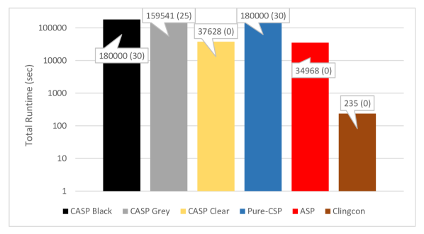
Figure 7: Performance on wseq domain: total times in logarithmic scale

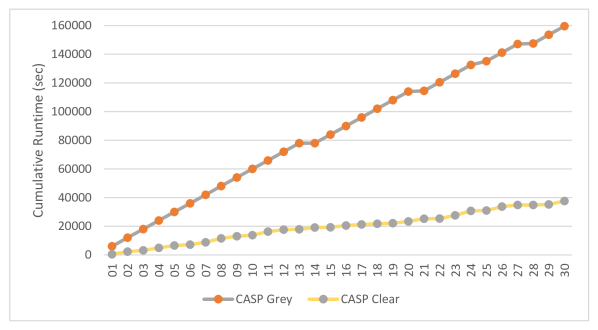
Figure 8: Performance on wseq domain: cumulative view (grey-box and clear-box)

The experimental comparison of the integration schemas was conducted on a computer with an Intel Core i7 processor at 3GHz and running Fedora Core 16. The memory limit for each process and the timeout were set to $1$ GB RAM and $6,000$ seconds respectively. A single processor core was used for every experiment.

The version of ezcsp used in the experiments was 1.6.20b49. This version implements the black-box, grey-box, and clear-box integration schemas, when suitable API interfaces are available in the base solver. One answer set solver that provides such interfaces is cmodels, which for this reason was chosen as base solver for the experiments. It is worth noting that the development of the API in cmodels was greatly facilitated by the API provided by minisat v. 1.12b supporting non-clausal constraints Eén and Sörensson (2003) (minisat forms the main inference mechanism of cmodels). In the experiments, we used cmodels version 3.83 as the base solver and bprolog 7.4 as the theory solver. Answer set solver cmodels 3.83 (with the inference mechanism of minisat v. 1.12b) was also used for the experiments with the pure-ASP encodings. Unless otherwise specified, for all solvers we used their default configurations.

The executables used in the experiments and the encodings can be downloaded, respectively, from

• http://www.mbal.tk/ezcsp/int_schemas/ezcsp-binaries.tgz,
  and

• http://www.mbal.tk/ezcsp/int_schemas/experiments.tgz.

In order to provide a frame of reference with respect to the state of the art in CASP, the results also include performance information for clingcon 2.0.3 on the true-CASP encodings adapted to the language of clingcon. We conjecture that the choice of constraint solver by clingcon (namely, gecode) together with theory propagation is the reason for clingcon’s better performance in a number of the experiments. Yet, in the context of our experiments, the performance of clingcon w.r.t. ezcsp is irrelevant. Our work is a comparative study of the impact of the different integration schemas for a fixed selection of a base and theory solver pair. System ezcsp provides us with essential means to perform this study.

In all figures presented: CASP Black, CASP Grey, CASP Clear denote ezcsp implementing respectively black-box, grey-box and clear-box, and running a true-CASP encoding; Pure-CSP denotes ezcsp implementing black-box running a pure-CSP encoding (note that for pure-CSP encodings there is no difference in performance between the integration schemas); ASP denotes cmodels running a pure-ASP encoding; Clingcon denotes clingcon running a true-CASP encoding. Each configuration is associated with the same color in all figures. A pattern is applied to the filling of the bars whenever the bar goes off-chart. The numbers in the overlaid boxes report the time in seconds and, in parentheses, the total number of timeouts and out-of-memory.

We begin our analysis with wseq (Figures 7 and 8). The total times across all the instances for all solvers/encodings pairs considered are shown in Figure 7. Because of the large difference between best and worst performance, a logarithmic scale is used. For uniformity of presentation, in the charts out-of-memory conditions and timeouts are both rendered as out-of-time results. The instances used in the experiments are the 30 instances available via aspcomp. Interestingly, answer set solver cmodels on the pure-ASP encoding has excellent performance, comparable to the best performance obtained with CASP encodings by ezcsp. Of the CASP encodings, the true-CASP encoding running in black-box times out on every instance. Figure 8 thus focuses on the cumulative run times of clear-box and grey-box (on the true-CASP encoding). The numbers on the horizontal axis identify the instances, while the vertical axis is for the cumulative run time, that is, the value for instance $n$ is the sum of the run times for instances $1\ldots n$. Cumulative times were chosen for the per-instance figures because they make for a more readable chart when there is large variation between the run times for the individual instances. As shown in Figure 8, the true-CASP encoding running in clear-box performs substantially better than grey-box. This demonstrates that, for this domain, the tight integration schema has an advantage.

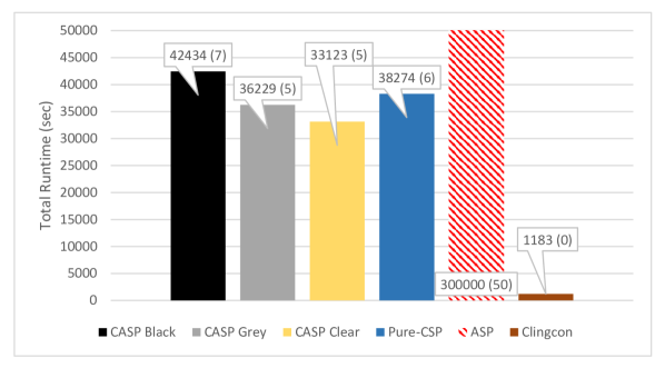
Figure 9: Performance on is domain, easy instances: total times (ASP encoding off-chart)

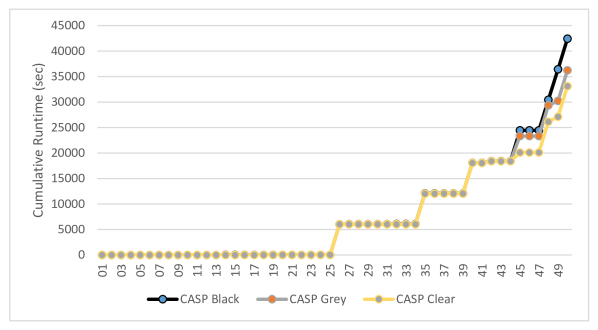
Figure 10: Performance on is domain, easy instances: cumulative view

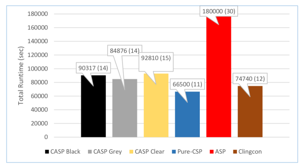
Figure 11: Performance on is domain, hard instances: overall view

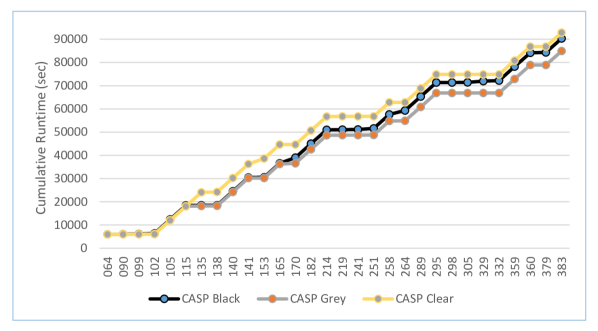
Figure 12: Performance on is domain, hard instances: cumulative view

In case of the is domain we considered two sets of experiments. In the first one (Figures 9 and 10), we used the 50 official instances from aspcomp. We refer to these instances as easy, since the corresponding run times are rather small. Figure 9 provides a comparison of the total times. Judging by the total times, tight integration schemas appear to have an advantage, allowing the true-CASP encoding to outperform the pure-CSP encoding. As one might expect, the best performance for the true-CASP encoding is from the clear-box integration schema. In this case the early pruning of the search space made possible by the clear-box architecture seems to yield substantial benefits. As expected, grey-box is also faster than black-box, while cmodels on the pure-ASP encoding runs out of memory in all the instances.

The second set of experiments for the is domain (Figures 11 and 12) consists of $30$ instances that we generated to be substantially more complex than the ones from aspcomp, and that are thus called hard. As discussed below, this second set of experiments reveals a remarkable change in the behavior of solver/encodings pairs when the instances require more computational effort. The process we followed to generate the $30$ hard instances consisted in (1) generating randomly $500$ fresh instances; (2) running the true-CASP encoding with the grey-box integration schema on them with a timeout of $300$ seconds; (3) selecting randomly, from those, $15$ instances that resulted in timeout and $15$ instances that were solved in $25$ seconds or more. The numerical parameters used in the process were selected with the purpose of identifying more challenging instances than those from the easy set and were based on the results on that set. The execution times reported in Figure 11 clearly indicate the level of difficulty of the selected instances (once again, cmodels runs out of memory). Remarkably, these more difficult instances are solved more efficiently by the pure-CSP encoding that relies only on the CSP solver. In fact, the pure-CSP encoding outperforms every other method of computation (including clingcon on true-CASP encoding). More specifically, solving the instances with the true-CASP encoding takes between $30\%$ and $50\%$ longer than with the pure-CSP encoding. This was not the isolated effect of a few instances, but rather a constant pattern throughout the experiment. A possible explanation for this phenomenon is that domain is is overall best suited to the CSP solving procedures. It seems natural for the difference in performance to become more evident as the problem instances become more challenging, when other factors such as overhead play less of a role. This conjecture is compatible with the difference in performance observed earlier on the easy instances.

Another remarkable aspect highlighted by Figure 12 is that clear-box is outperformed by grey-box. This is the opposite of what was observed on the easy instances and highlights the fact that there is no single-best integration schema, even when one focuses on true-CASP encodings. We hypothesize this to be due to the nature of the underlying scheduling problem, which is hard to solve, but whose relaxations (obtained by dropping one or more constraints) are relatively easy. Under these conditions, the calls executed by clear-box to the theory solver are ineffective at pruning the search space and incur a non-negligible overhead. (The performance of clingcon is likely affected by the same behavior.) In grey-box, on the other hand, no time is wasted trying to prune the search space of the base solver, and all the time spent in the theory solver is dedicated to solving the final CSP. The performance of black-box is likely due to the minor efficiency of its integration schema compared to grey-box.

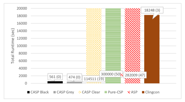
Figure 13: Performance on rf domain: total times (detail of 0-20,000sec execution time range, clear-box and pure-ASP off-chart)

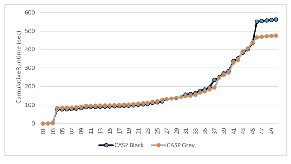
Figure 14: Performance on rf domain: cumulative view (black-box and grey-box)

The final experiment focuses on the rf domain (Figures 13 and 14). The instances used in this experiment are the 50 official instances from aspcomp. The total execution times are presented in Figure 13. Although the instances for this domain are comparatively easy, as suggested by the black-box and grey-box times, some of the configurations have high total execution times. The clear-box encoding is also off-chart, due to timeouts on $19$ instances. This is a substantial difference in performance compared to the other true-CASP configurations, upon which we expand later in this section. Surprisingly, the total time of clingcon is also close to off-chart. Upon closer inspection, we have found this to be due to $3$ instances for which clingcon runs out of memory. This is an interesting instance of the trade-off between speed of execution and performance stability, considering that on the other instances clingcon is very fast. The per-instance execution times for grey-box and black-box are detailed in Figure 14. The figure highlights the very similar performance of the two schemas, with black-box losing only in the final 10% of the instances in spite of its higher overhead. This is likely due to the simplicity of the rf problem: most extended answer sets can be found with little backtracking between base and theory solver, and thus the difference between the two schemas has little bearing on the execution times. Similarly to the hard instances of the is domain, the better performance of black-box and grey-box in comparison to clear-box can be explained by the fact that, in this domain, frequent checks with the theory solver add overhead but are overall ineffective at pruning the search.

8 A Brief Account on Related Systems

In the introduction we mentioned solvers acsolver Mellarkod et al. (2008), clingcon Gebser et al. (2009), idp Wittocx et al. (2008), inca Drescher and Walsh (2011), dingo Janhunen et al. (2011), mingo Liu et al. (2012), aspmt2smt Bartholomew and Lee (2014), and ezsmt Susman and Lierler (2016). In this section we briefly remark on this variety of CASP systems. This is not intended as a detailed comparison between the systems, but as a quick summary.

At a high-level abstraction, one may easily relate the architectures of the clingcon, acsolver, idp, and inca to that of ezcsp. Given a CASP program, all of these systems first utilize an answer set solver to compute a part of an answer set for an asp-abstraction and then utilize a constraint programming system to solve a resulting csp-abstraction. All of these systems implement the clear-box integration schema. Table 2 provides a summary of base solvers and theory solvers utilized by them.

	Base Solver	Theory Solver
acsolver	smodels Simons et al. (2002)	constraint logic programming systems
clingcon	clasp Gebser et al. (2007)	gecode Schulte and Stuckey (2008)
idp	minisat(id) Cat et al. (2014)	gecode Schulte and Stuckey (2008)
inca	clasp Gebser et al. (2007)	its own CP solver

Table 2: Solvers used by state-of-the-art CASP systems

A few remarks are due. Unlike its peers, acsolver does not implement learning as its base solver smodels does not support this technique. The fact that system inca implements its own CP solver, or, in other words, a set of its in house CP-based propagators allows this system to take advantage of some sophisticated techniques stemming from CP. In particular, it implements so called “lazy nogood generation”. This technique allows one to transfer some of the information stemming from CP-based propagations into a propositional logic program extending the original input to a base solver. We also note that the latest version of clingcon, as well, bypasses the use of gecode by implementing its own CP-based propagators. All of the above systems are focused on finite domain integer linear constraints. Some of them allow for global constraints.

System dingo translates CA programs into SMT modulo difference logic formulas and applies the SMT solver z3 De Moura and Bjørner (2008) to find their models. Rather than arbitrary integer linear constraints, the system only handles those that fall into the class of difference logic. On the other hand, the system does not pose the restriction of finite domain. The ezsmt Susman and Lierler (2016) solver and the aspmt2smt Bartholomew and Lee (2014) solvers utilize SMT solvers to process CA programs. Both of these systems may only deal with tight programs. They allow for arbitrary integer linear constraints. None of the SMT-based CASP solvers allow for global constraints in their programs due to the underlying solving technology.

Last but not least, the solver mingo translates CA programs into mixed integer programming expressions and then utilizes IBM ILOG cplex system to find solutions.

Susman and Lierler (Susman and Lierler (2016)) provide an experimental analysis of systems from all of the families mentioned.

9 Conclusions

In this paper, we have addressed in a principled way the integration of answer set solving techniques and constraint solving techniques in CASP solvers and, in particular, in the realm of the constraint answer set solver ezcsp. To begin, we defined logic programs with constraint atoms (CA programs). To bridge the ASP and the constraint programming aspects of such programs, we introduced the notions of asp-abstractions and csp-abstractions, which allow for a simple and yet elegant way of defining the extended answer sets of CA programs.

Next, we described the syntax of the CASP language used by the constraint answer set solver ezcsp, which we call ez. It is worth noting that this paper contains the first detailed and principled account of the syntax of the ez language. We relate programs written in the ezcsp language and CA programs. The tight relation between ez programs and CA programs makes it evident that the ez language is a full-fledged constraint answer set programming formalism. Recall that the ezcsp system originated as an attempt to provide a simple, flexible framework for modeling constraint satisfaction problems. This yields an interesting observation: constraint answer set programming can be seen as a declarative modeling framework utilizing constraint satisfaction solving technology.

In this paper we also drew a parallel between CASP and SMT. We used this connection to introduce three important kinds of integration of CASP solvers: black-box integration, grey-box integration, and clear-box integration. We introduced a graph-based abstract framework suitable for describing the ezcsp solving algorithm. The idea of using graph-based representations for backtrack-search procedures was pioneered by the SAT community. Compared to the use of pseudocode for describing algorithms, such a framework allows for simpler descriptions of search algorithms, and is well-suited for capturing the similarities and differences of the various configurations of ezcsp stemming from different integration schemas.

Finally, we presented an experimental comparison of the various integration schemas, using the implementation of ezcsp as a testbed. For the comparison, we used three challenging benchmark problems from the Third Answer Set Programming Competition – 2011  Calimeri et al. (2011). The experimental analysis takes into account how differences in the encoding of the solutions may influence overall performance by exploiting the components of the solver in different ways. The case study that we conducted clearly illustrates the influence that integration methods have on the behavior of hybrid systems. The main attractive feature of the black-box integration schema is the ease of inception of a new system. In realm of CASP, one may take existing off-the-shelf ASP and CSP tools and connect them together by simple intermediate translation functions. This facilitates fast implementation of a prototypical CASP solver. One can then move towards a grey-box or clear-box architecture in the hope of increased performance when a prototype system proves to be promising. Yet, our experiments demonstrate that different integration schemas may be of use and importance for different domain, and that, when it comes to performance, there is no single-best integration schema. Thus, systematic means ought to be found for facilitating building hybrid systems supporting various coupling mechanisms. Just as the choice of a particular heuristic for selecting decision literals is often configurable in SAT or ASP solvers via command line parameters, the choice of integration schema in hybrid systems should be configurable. Experimental results also indicate a strong need for theory propagation. Standard interfaces in both base and theory systems are required in order to easily build hybrid systems to support this feature.

Building clear and flexible APIs allowing for various types of interactions between the solvers seems a necessary step towards making the development of hybrid solvers effective. This work provides evidence for the need of an effort towards this goal. Many SAT solvers and SMT solvers already come with APIs that aim at facilitating extensions of these complex software systems. We argue for this practice to be adopted by other automated reasoning communities.

Finally, our study was performed in the realm of CASP technology, but it translates to SMT as well, given the discussed links between the two technologies. Incidentally, this also brings to the surface the importance of establishing means of effective communication between the two communities of constraint answer set programming and SMT solving.

Appendix A ez – The Language of ezcsp

The ez language is aimed at a convenient specification of a propositional ez-program $\mathcal{E}\mathchar 61\relax\langle E,\mathcal{A},\mathcal{C},\gamma,D\rangle$. To achieve this, the language supports an explicit specification of domains and variables, the use of non-ground rules, and a compact representation of lists in constraints. We begin by describing the syntax of the language. Next, we define a mapping from ez programs to propositional ez-programs.

Let $\Sigma_{\textsc{ez}}\mathchar 61\relax\langle C_{\textsc{ez}},V_{\textsc{ez}},F_{\textsc{ez}},R_{\textsc{ez}}\rangle$ be a signature, where $C_{\textsc{ez}},V_{\textsc{ez}},F_{\textsc{ez}}$, and $R_{\textsc{ez}}$ denote pairwise disjoint sets of constant symbols, non-constraint variable symbols, function symbols, and relation symbols respectively. Set $C_{\textsc{ez}}$ includes symbols for integers and pre-defined constants ($fd$, $q$, $r$), denoting CSP domains. We use common convention in logic programming and denote non-constraint variable symbols in $V_{\textsc{ez}}$ by means of upper case letters. Function and relation symbols are associated with a non-negative integer called arity. The arity of function symbols is always greater than $0$. Set $F_{\textsc{ez}}$ includes pre-defined symbols that intuitively correspond to arithmetic operators (e.g., $\mathchar 43\relax$), reified arithmetic connectives (e.g., $\mathchar 60\relax$, $\mathchar 61\relax$), reified logical connectives (see Table 3), list delimiters ($[$ and $]$) and names of global constraints (discussed later in this section). Set $R_{\textsc{ez}}$ contains pre-defined symbols $cspdomain$, $cspvar$, $required$.

The notions of terms, atoms, literals, and rules are defined over $\Sigma_{\textsc{ez}}$ similarly to ASP, although the notion of term is slightly expanded. Specifically, a term over signature $\Sigma_{\textsc{ez}}\mathchar 61\relax\langle C_{\textsc{ez}},V_{\textsc{ez}},F_{\textsc{ez}},R_{\textsc{ez}}\rangle$ is defined as:

1. a constant symbol from $C_{\textsc{ez}}$.

2. a variable symbol from $V_{\textsc{ez}}$.

3. an expression of the form

   $$f(t_{1},\ldots,t_{k}),$$ (16)

   where $f$ is a function symbol in $F_{\textsc{ez}}$ of arity $k$ and $\langle t_{1},\ldots,t_{k}\rangle$ are terms from cases 1–3 (If a function symbol is a pre-defined arithmetic operator, arithmetic connective, or logical connective, then common infix notation is used.)

4. an extensional list, i.e., an expression of the form $[t_{1},t_{2},\ldots,t_{k}]$ where $t_{i}$’s are terms from cases 1–3.

5. an intensional list, i.e., an expression of the form $[g/k]$ where $g\in F_{\textsc{ez}}$ or (with slight abuse of notation) $g\in R_{\textsc{ez}}$ and $k$ is an integer.

6. a global constraint, i.e., an expression of the form $f(\lambda_{1},\lambda_{2},\ldots,\lambda_{k})$, where $f\in F_{\textsc{ez}}$ and each $\lambda_{i}$ is a list.

Connective	Constraint Domain
$\lor$	Disjunction
$\land$	Conjunction
$\backslash$	Exclusive disjunction
$\leftarrow$ or $\rightarrow$	Implication
$\leftrightarrow$	Equivalence
$!$	Negation

Table 3: ez Logical Connectives

Pre-defined arithmetic and logical connectives from $F_{\textsc{ez}}$ are dedicated to the specification of constraints. The connectives are reified to enable their use within atoms of the form $required(\beta)$. Furthermore, the logical connectives enable the specification of so called “reified constraints” such as:

$$x\geq 12\lor y\mathchar 60\relax 3,$$ (17)

which specifies that either constraint $x\geq 12$ or constraint $y\mathchar 60\relax 3$ should be satisfied by a solution to a problem containing reified constraint (17).

An ez program is a pair $\langle\Sigma_{\textsc{ez}},\Pi\rangle$, where $\Pi$ is a set of rules over signature $\Sigma_{\textsc{ez}}$. Every ez program is required to contain exactly one fact, whose head is $cspdomain(fd)$, $cspdomain(q)$, or $cspdomain(r)$. Following common practice, we denote a program simply by the set of its rules, and let the signature be implicitly defined.

Similarly to ASP, a non-ground rule is a rule containing one or more non-constraint variables. A non-ground rule is interpreted as a shorthand for the set of propositional (ground) rules obtained by replacing every non-constraint variable in the rule by suitable terms not containing non-constraint variables. The process of replacing non-ground rules by their propositional counterparts is called grounding and is well understood in ASP Gebser et al. (2007); Calimeri et al. (2008). For this reason, in the rest of this section we focus on ground ez programs.

We now define a mapping from a (ground) ez program $\Pi$ to a propositional ez-program $\mathcal{E}\mathchar 61\relax\langle E,\mathcal{A},\mathcal{C},\gamma,D\rangle$. We assume that $\gamma$, a function from $\mathcal{C}$ to constraints, is defined along the lines of Section 2.2 and given. Recall that only one fact formed from relation $cspdomain$ is allowed in a program $\Pi$. The fact’s head is mapped to the constraint domain $D$ by mapping $\mu_{D}$:

• $\displaystyle\hskip 25.00003pt{\mu_{D}(\Pi)\mathchar 61\relax\left\{\begin{array}[]{cl}\mathcal{FD}\mbox{ (finite domains)}&\mbox{ if }cspdomain(fd)\mathbin{\cdot}\in\Pi\\ \mathcal{Q}&\mbox{ if }cspdomain(q)\mathbin{\cdot}\in\Pi\\ \mathcal{R}&\mbox{ if }cspdomain(r)\mathbin{\cdot}\in\Pi\\ \end{array}\right\mathbin{\cdot}}$

Atoms formed from relation $cspvar$ specify the set $\mathcal{V}_{{\mathcal{P}_{\mathcal{E}}}}$ of variables (recall that $\mathcal{V}_{{\mathcal{P}_{\mathcal{E}}}}$ is the set of constraint variables that appear in csp-abstractions corresponding to $\mathcal{E}$). The corresponding atoms take two forms, $cspvar(v)$ and $cspvar(v,l,u)$, where $v$ is a term from $\Sigma_{\textsc{ez}}$ and $l$, $u$ belong to $C_{\textsc{ez}}\cap D$. The latter form allows one to provide a range for the variable. Specifically, set $\mathcal{V}_{{\mathcal{P}_{\mathcal{E}}}}$ is obtained from facts containing the above atoms as follows:

• $\displaystyle\hskip 25.00003pt{\mathcal{V}_{{\mathcal{P}_{\mathcal{E}}}}\mathchar 61\relax\{v\,|\,cspvar(v)\mathbin{\cdot}\in\Pi\mbox{ or }cspvar(v,l,u)\mathbin{\cdot}\in\Pi\}\mathbin{\cdot}}$

The constraints that specify the range of the variables are generated by mapping $\mu_{V}$:

• $\displaystyle\hskip 25.00003pt{\begin{array}[]{ll}\mu_{V}(\Pi)\mathchar 61\relax&\{required(v\geq l)\mathbin{\cdot}\,|\,cspvar(v,l,u)\mathbin{\cdot}\in\Pi\}\ \ \cup\\ &\{required(v\leq u)\mathbin{\cdot}\,|\,cspvar(v,l,u)\mathbin{\cdot}\in\Pi\}\mathbin{\cdot}\end{array}}$

Next, we address the specification of lists. Let us begin by introducing some needed terminology. If a term is of the form (16) then we refer to $f$ as a functor and to $\langle t_{1},\ldots,t_{k}\rangle$ as its arguments. For an atom of the form $r(t_{1},\ldots,t_{k})$ we say that $r$ is its relation and $\langle t_{1},\ldots,t_{k}\rangle$ are its arguments. The expression $terms(f,k,\langle t_{1},t_{2},\ldots t_{m}))$ (with $0\leq m\leq k$) denotes the set of terms from $\Sigma_{\textsc{ez}}$ formed by functor $f$ that have arity $k$ and whose arguments have prefix $\langle t_{1},t_{2},\ldots,t_{m}\rangle$. The expression $atoms(r,k,\langle t_{1},\ldots,t_{k}\rangle)$ denotes the set of atoms formed by relation $r$ that have arity $k$ and whose arguments have prefix $\langle t_{1},t_{2},\ldots,t_{m}\rangle$. The expression $facts(\Pi)$ denotes the facts in $\Pi$. Finally, given a set $S$, $lexord(S)$ denotes a list $[e_{1},e_{2},\ldots,e_{n}]$ enumerating the elements of $S$ in such a way that $e_{i}\leq e_{i\mathchar 43\relax 1}$ (where $\leq$ denotes lexicographic ordering). We can now define mappings $\lambda_{v}$ and $\lambda_{r}$ from the two forms of intensional lists to corresponding extensional lists:

• Given an expression of the form $[f(t_{1},t_{2},\ldots,t_{m})/k]$, where $f\in F_{\textsc{ez}}$, $k$ is an integer from $C_{\textsc{ez}}$, $t_{i}$’s are terms, and $0\leq m\leq k$, its extensional representation is the list:

  • $\displaystyle\hskip 25.00003pt{\lambda_{v}([f(t_{1},t_{2},\ldots,t_{m})/k])\mathchar 61\relax lexord(terms(f,k,\langle t_{1},t_{2},\ldots,t_{m}\rangle)\cap\mathcal{V}_{{\mathcal{P}_{\mathcal{E}}}})}$

  of all variables with functor $f$, arity $k$, and whose arguments have prefix $\langle t_{1},t_{2},\ldots,t_{m}\rangle$. For example, given a set of variables

  $$X_{1}\mathchar 61\relax\{v(1),v(2),v(3),w(a,1),w(a,2),w(b,1)\},$$

  the expression $[w(a)/2]$ denotes the list $\lambda_{v}(w,2,\langle a\rangle)\mathchar 61\relax[w(a,1),w(a,2)]$. When $m\mathchar 61\relax 0$, the expression is abbreviated $[f/k]$. For instance, given set $X_{1}$ as above, the expression $[v/1]$ denotes $[v(1),v(2),v(3)]$.

• Consider an expression $[r(t_{1},t_{2},\ldots,t_{m})/k]$, where $r$ is not a pre-defined relation from $R_{\textsc{ez}}$ and $0\leq m\leq k$. Let $[a_{1},a_{2},\ldots,a_{n}]$ denote list $lexord(facts(\Pi)\cap atoms(r,k,\langle t_{1},\ldots,t_{m}\rangle))$ and let $\alpha^{k}_{i}$ denote the $k^{th}$ argument of $a_{i}$. Then, the extensional representation, $\lambda_{r}([r(t_{1},t_{2},\ldots,t_{m})/k])$, of $[r(t_{1},t_{2},\ldots,t_{m})/k]$ is:

  • $\displaystyle\hskip 25.00003pt{\lambda_{r}([r(t_{1},t_{2},\ldots,t_{m})/k])\mathchar 61\relax[\alpha_{1}^{k},\alpha_{2}^{k},\ldots,\alpha_{n}^{k}]\mathbin{\cdot}}$

  For example, given a relation $r^{\prime}$ defined by facts $r^{\prime}(a,1,3),r^{\prime}(a,2,1),r^{\prime}(b,5,7)$, the expression $[r^{\prime}(a)/3]$ denotes the list $[3,1]$ and the expression $[r^{\prime}(a,2)/3]$ denotes $[1]$. Similarly to the previous case, when the list of arguments is empty, the expression can be abbreviated as $[r/k]\mathbin{\cdot}$ For instance, given a relation $r^{\prime\prime}$ for which we are given facts $r^{\prime\prime}(a,3),r^{\prime\prime}(b,1),r^{\prime\prime}(c,2)$, the expression $[r^{\prime\prime}/2]$ denotes $\langle 3,1,2\rangle$.

As a practical example of the use of intensional lists, suppose that, above, relation $r^{\prime\prime}$ denotes the amount of resources required for a job and suppose that we are given facts $d(a,1),d(b,1),d(c,1)$, specifying that jobs $a$, $b$, $c$ have duration $1$. Additionally, variables $st(a)$, $st(b)$, $st(c)$ represent the start time of the jobs. A cumulative constraint for this scenario can be written as

• $\displaystyle\hskip 25.00003pt{required(cumulative([st/1],[d/2],[r^{\prime\prime}/2],4)),}$

which is an abbreviation of

• $\displaystyle\hskip 25.00003pt{required(cumulative([st(a),st(b),st(c)],[1,1,1],[3,2,1],4))\mathbin{\cdot}}$

and means that values should be assigned to variables $st(a),st(b),st(c)$ so that each job, of duration $1$ and requiring amounts of resources $3,2,1$ respectively, can be executed on a machine that can provide at most $4$ resources at any given time.

Next, let $\mu_{R}$ be a function that maps an atom of the form $required(\beta)$ to an atom $required(\beta^{\prime})$ by:

• Replacing every occurrence of $[f(t_{1},\ldots,t_{m})/k]$ in $\beta$ by $\lambda_{v}([f(t_{1},\ldots,t_{m})/k])$;

• Replacing every occurrence of $[r(t_{1},\ldots,t_{m})/k]$ in $\beta$ by $\lambda_{r}([f(t_{1},\ldots,t_{m})/k])$.

The mapping is easily extended to rules and to programs as follows:

• $\displaystyle\hskip 25.00003pt{\mu_{R}(a\leftarrow B\ldotp)\mathchar 61\relax\left\{\begin{array}[]{ll}\mu(a)\leftarrow B\ldotp&\mbox{if $a$ is of the form $required(\beta)$}\\ a\leftarrow B\ldotp&\mbox{otherwise}\end{array}\right\mathbin{\cdot}}$

where $B$ denotes the body of a rule.

• $\displaystyle\hskip 25.00003pt{\mu_{R}(\Pi)\mathchar 61\relax\bigcup_{r\in\Pi}\mu_{R}(r)}$

Finally, let $\mu_{\mathcal{A}}(\Pi)$ and $\mu_{\mathcal{C}}(\Pi)$ denote mappings from $\Pi$ to alphabets $\mathcal{A}$ and $\mathcal{C}$, which are straightforward given the above construction. Thus, given an ez program $\Pi$, the corresponding propositional ez-program is:

• $\displaystyle\hskip 25.00003pt{\mathcal{E}(\Pi)\mathchar 61\relax\langle\ \mu_{V}(\Pi)\cup\mu_{R}(\Pi),\ \mu_{\mathcal{A}}(\Pi),\ \mu_{\mathcal{C}}(\Pi),\ \gamma,\ \mu_{D}(\Pi)\ \rangle\mathbin{\cdot}}$

A.1 Global Constraints in Language ez

The global constraints supported by the ez language include:

• $all\_dif\!ferent(V)$, where $V$ is a list of variables. This constraint, available only in the $fd$ domain, ensures that all the variables in $V$ are assigned unique values. Typically, the implementation of the corresponding algorithm found in constraint solvers is incomplete. Global constraint $all\_distinct(V)$, which provides a complete implementation of the algorithm, is also supported.

• $assignment(X,Y)$, where $X$ and $Y$ are lists of $n$ variables whose domain is $1\mathbin{\cdot}\mathbin{\cdot}n$. The constraint is satisfied if, for every $i,j$, $X_{i}\mathchar 61\relax j$ if and only if $Y_{j}\mathchar 61\relax i$.

• $circuit(V)$, where $V$ is a list of $n$ variables whose domain is $1\mathbin{\cdot}\mathbin{\cdot}n$. The constraint is satisfied by an assignment $V_{1}\mathchar 61\relax v_{1}$, $V_{2}\mathchar 61\relax v_{2}$, $\ldots$, $V_{n}\mathchar 61\relax v_{n}$ if the directed graph with nodes $1\ldots n$ and arcs $\langle 1,v_{1}\rangle$, $\langle 2,v_{2}\rangle$, $\ldots$, $\langle n,v_{n}\rangle$ forms a Hamiltonian cycle.

• $count(M,V,\circ,E)$, where $M$ is an integer or variable, $V$ a list of variables, $\circ$ an arithmetic comparison operator, and $E$ an integer or variable. This constraint is satisfied if the number, $c$, of elements of $V$ that equal $M$ is such that $c\circ E$.

• $cumulative(S,D,R,L)$, where $S$ is a list of variables, $D$ and $R$ are lists of non-negative integers matching the length of $S$, and $L$ is an integer or a variable. This constraint, which is only available in the $fd$ domain, is typically used in scheduling problems. In that context, $S$ represent the start times of a set of jobs, $D$ provides the duration of those jobs, and $R$ the resources they require. $L$ is the amount of resources available at any time step. Intuitively, the constraint assigns start times to the jobs so that, at any time, no more than an amount $L$ of resources is used.

• $disjoint2(X,W,Y,H)$, where $X,Y$ are lists of variables and $W,H$ are lists of integers defining the coordinates and dimensions of rectangles. For example, if $X\mathchar 61\relax[x_{1},\ldots]$, $Y\mathchar 61\relax[y_{1},\ldots]$, $W\mathchar 61\relax[w_{1},\ldots]$, $H\mathchar 61\relax[h_{1},\ldots]$, one of the rectangles they describe has top-left vertex $\langle x_{1},y_{1}\rangle$ and bottom-right vertex $\langle x_{1}\mathchar 43\relax w_{1},y_{1}\mathchar 43\relax h_{1}\rangle$. This constraint is only available in the $fd$ domain, and assigns values to the variables so that the corresponding rectangles do not overlap.

• $element(I,V,E)$, where $I$ is an integer or variable, $V$ a list of variables, and $E$ an integer or variable. This constraint is satisfied if the $I^{th}$ element of $V$ is $E$.

• $minimum(M,V)$ and $maximum(M,V)$, where $M$ is a variable or integer and $V$ is a list of variables. These constraints are satisfied if minimum or maximum of $V$ equals $M$.

• $scalar\_product(C,X,\circ,E)$, where $C$ is a list of integers, $X$ is a list of variables, $\circ$ is an arithmetic comparison operator, and $E$ is an integer or variable. The intuitive meaning of this constraint is that the scalar product, $p$, of the elements of $C$ and $X$ must be such that $p\circ E$.

• $serialized(S,D)$, where $S$ is a list of variables and $D$ is a list of integers, intuitively denoting start time and duration of jobs. The constraint assigns start times to the jobs so that their execution does not overlap, and can be viewed as a special case of $cumulative$.

• $sum(V,\circ,E)$, where $V$ is a list of variables, $\circ$ an arithmetic comparison operator, and $E$ is an integer or a variable. This constraint assigns value to the variables so that $(\sum_{v\in V}v)\circ E$ is satisfied.

References

- Anger et al. (2006) Anger, C., Gebser, M., Janhunen, T., and Schaub, T. 2006. What’s a head without a body? In Proceedings of the European Conference on Artificial Intelligence (ECAI’06). 769–770.
- Balduccini (2009a) Balduccini, M. 2009a. Representing constraint satisfaction problems in answer set programming. In ICLP09 Workshop on Answer Set Programming and Other Computing Paradigms (ASPOCP09).
- Balduccini (2009b) Balduccini, M. 2009b. Representing constraint programming. in: Proceedings of ICLP Workshop on Answer Set Programming and Other Computing Paradigms (ASPOCP), https://www.mat.unical.it/{A}{S}{POCP}09/%.
- Balduccini (2011) Balduccini, M. 2011. Industrial-size scheduling with ASP+CP. In 11th International Conference on Logic Programming and Nonmonotonic Reasoning (LPNMR11), J. P. Delgrande and W. Faber, Eds. Lecture Notes in Artificial Intelligence (LNCS), vol. 6645. Springer Verlag, Berlin, 284–296.
- Balduccini and Lierler (2012) Balduccini, M. and Lierler, Y. 2012. Practical and methodological aspects of the use of cutting-edge ASP tools. In Fourteenth International Symposium on Practical Aspects of Declarative Languages (PADL 2012), C. Russo and N.-F. Zhou, Eds. Number 7149 in Lecture Notes in Artificial Intelligence (LNCS). Springer Verlag, Berlin, 78–92.
- Bartholomew and Lee (2014) Bartholomew, M. and Lee, J. 2014. System aspmt2smt: Computing ASPMT theories by SMT solvers. In European Conference on Logics in Artificial Intelligence, JELIA. Springer, 529–542.
- Brewka et al. (2011) Brewka, G., Eiter, T., and Truszczyński, M. 2011. Answer set programming at a glance. Communications of the ACM 54(12), 92–103.
- Calimeri et al. (2007) Calimeri, F., Cozza, S., and Ianni, G. 2007. External sources of knowledge and value invention in logic programming. Annals of Mathematics and Artificial Intelligence 50, 3-4, 333–361.
- Calimeri et al. (2008) Calimeri, F., Cozza, S., Ianni, G., and Leone, N. 2008. Computable functions in ASP: theory and implementation. In Proceedings of International Conference on Logic Programming (ICLP), M. Garcia de la Banda and E. Pontelli, Eds. Lecture Notes in Artificial Intelligence (LNCS), vol. 5366. Springer Verlag, Berlin, 407–424.
- Calimeri et al. (2011) Calimeri, F., Ianni, G., Ricca, F., Alviano, M., Bria, A., Catalano, G., Cozza, S., Faber, W., Febbraro, O., Leone, N., Manna, M., Martello, A., Panetta, C., Perri, S., Reale, K., Santoro, M. C., Sirianni, M., Terracina, G., and Veltri, P. 2011. The third answer set programming competition: Preliminary report of the system competition track. In Proceedings of the International Conference on Logic Programming and Nonmonotonic Reasoning (LPNMR). Springer-Verlag, Berlin, Heidelberg, 388–403.
- Carlsson and Mildner (2012) Carlsson, M. and Mildner, P. 2012. SICStus Prolog-the first 25 years. Theory Pract. Log. Program. 12, 1-2 (Jan.), 35–66.
- Cat et al. (2014) Cat, B. D., Bogaerts, B., and Denecker, M. 2014. MiniSAT(ID) for satisfiability checking and constraint solving. In ALP newsletter feautured article.
- Davis et al. (1962) Davis, M., Logemann, G., and Loveland, D. 1962. A machine program for theorem proving. Communications of the ACM 5(7), 394–397.
- De Moura and Bjørner (2008) De Moura, L. and Bjørner, N. 2008. Z3: An efficient SMT solver. In Proceedings of the Theory and Practice of Software, 14th International Conference on Tools and Algorithms for the Construction and Analysis of Systems. 337–340.
- Denecker et al. (2009) Denecker, M., Vennekens, J., Bond, S., Gebser, M., and Truszczyński, M. 2009. The second answer set programming system competition. In Proceedings of the International Conference on Logic Programming and Nonmonotonic Reasoning (LPNMR), E. Erdem, F. Lin, and T. Schaub, Eds. Lecture Notes in Artificial Intelligence (LNCS), vol. 5753. Springer Berlin Heidelberg, Berlin, Heidelberg.
- Dovier et al. (2011) Dovier, A., Formisano, A., and Pontelli, E. 2011. Logic Programming, Knowledge Representation, and Nonmonotonic Reasoning: Essays Dedicated to Michael Gelfond on the Occasion of His 65th Birthday. Lecture Notes in Artificial Intelligence (LNCS). Springer Verlag, Berlin, Chapter Perspectives on Logic-based Approaches for Reasoning, 259–279.
- Drescher and Walsh (2011) Drescher, C. and Walsh, T. 2011. A translational approach to constraint answer set solving. Theory and Practice of Logic programming (TPLP) 10, 4-6, 465–480.
- Eén and Biere (2005) Eén, N. and Biere, A. 2005. Effective preprocessing in SAT through variable and clause elimination. In SAT.
- Eén and Sörensson (2003) Eén, N. and Sörensson, N. 2003. An extensible SAT-solver. In SAT.
- Eiter et al. (2005) Eiter, T., Ianni, G., Schindlauer, R., and Tompits, H. 2005. A uniform integration of higher-order reasoning and external evaluations in answer set programming. In Proceedings of International Joint Conference on Artificial Intelligence (IJCAI). Professional Book Center, 90–96.
- Elkabani et al. (2004) Elkabani, I., Pontelli, E., and Son, T. C. 2004. Smodels with CLP and its applications: A simple and effective approach to aggregates in ASP. In ICLP, B. Demoen and V. Lifschitz, Eds. Lecture Notes in Computer Science, vol. 3132. Springer, 73–89.
- Ferraris and Lifschitz (2005) Ferraris, P. and Lifschitz, V. 2005. Weight constraints as nested expressions. Theory and Practice of Logic Programming 5, 45–74.
- Gebser et al. (2007) Gebser, M., Kaufmann, B., Neumann, A., and Schaub, T. 2007. Conflict-driven answer set solving. In Proceedings of 20th International Joint Conference on Artificial Intelligence (IJCAI’07). MIT Press, 386–392.
- Gebser et al. (2007) Gebser, M., Liu, L., Namasivayam, G., Neumann, A., Schaub, T., and Truszczyński, M. 2007. The first answer set programming system competition. In Proceedings of the International Conference on Logic Programming and Nonmonotonic Reasoning (LPNMR), C. Baral, G. Brewka, and J. Schlipf, Eds. Lecture Notes in Artificial Intelligence (LNCS), vol. 4483. Springer Berlin Heidelberg, Berlin, Heidelberg, 3–17.
- Gebser et al. (2009) Gebser, M., Ostrowski, M., and Schaub, T. 2009. Constraint answer set solving. In Proceedings of 25th International Conference on Logic Programming (ICLP), P. M. Hill and D. S. Warren, Eds. Lecture Notes in Artificial Intelligence (LNCS), vol. 5649. Springer Berlin Heidelberg, Berlin, Heidelberg, 235–249.
- Gebser et al. (2007) Gebser, M., Schaub, T., and Thiele, S. 2007. Gringo: A new grounder for answer set programming. In Logic Programming and Nonmonotonic Reasoning, C. Baral, G. Brewka, and J. Schlipf, Eds. Lecture Notes in Computer Science, vol. 4483. Springer Berlin Heidelberg, 266–271.
- Gelfond and Lifschitz (1998) Gelfond, M. and Lifschitz, V. 1998. Action languages141414http://www.ep.liu.se/ea/cis/1998/016/. Electronic Transactions on Artificial Intelligence 3, 195–210.
- Giunchiglia et al. (2008) Giunchiglia, E., Leone, N., and Maratea, M. 2008. On the relation among answer set solvers. Ann. Math. Artif. Intell. 53, 1-4, 169–204.
- Giunchiglia et al. (2006) Giunchiglia, E., Lierler, Y., and Maratea, M. 2006. Answer set programming based on propositional satisfiability. Journal of Automated Reasoning 36, 345–377.
- Gomes et al. (2008) Gomes, C. P., Kautz, H., Sabharwal, A., and Selman, B. 2008. Satisfiability solvers. In Handbook of Knowledge Representation, F. van Harmelen, V. Lifschitz, and B. Porter, Eds. Elsevier, 89–134.
- Jaffar and Maher (1994) Jaffar, J. and Maher, M. J. 1994. Constraint logic programming: a survey. The Journal of Logic Programming 19–20, Supplement 1, 0, 503 – 581. Special Issue: Ten Years of Logic Programming.
- Janhunen et al. (2011) Janhunen, T., Liu, G., and Niemelä, I. 2011. Tight integration of non-ground answer set programming and satisfiability modulo theories. In Working notes of the 1st Workshop on Grounding and Transformations for Theories with Variables.
- Lee (2005) Lee, J. 2005. A model-theoretic counterpart of loop formulas. In Proceedings of International Joint Conference on Artificial Intelligence (IJCAI). Professional Book Center, 503–508.
- Lierler (2014) Lierler, Y. 2014. Relating constraint answer set programming languages and algorithms. Artificial Intelligence 207C, 1–22.
- Lierler et al. (2012) Lierler, Y., Smith, S., Truszczyński, M., and Westlund, A. 2012. Weighted-sequence problem: ASP vs CASP and declarative vs problem oriented solving. In Proceedings of the 14th International Symposium on Practical Aspects of Declarative Languages (PADL), C. V. Russo and N.-F. Zhou, Eds. Lecture Notes in Computer Science, vol. 7149. Springer Verlag, Berlin.
- Lierler and Truszczyński (2011) Lierler, Y. and Truszczyński, M. 2011. Transition systems for model generators — a unifying approach. Theory and Practice of Logic Programming, 27th Int’l. Conference on Logic Programming (ICLP’11) Special Issue 11, 4-5, 629–646.
- Lifschitz et al. (1999) Lifschitz, V., Tang, L. R., and Turner, H. 1999. Nested expressions in logic programs. Annals of Mathematics and Artificial Intelligence 25, 369–389.
- Liu et al. (2012) Liu, G., Janhunen, T., and Niemelä, I. 2012. Answer set programming via mixed integer programming. In Principles of Knowledge Representation and Reasoning: Proceedings of the 13th International Conference. AAAI Press, 32–42.
- Marek and Truszczyński (1999) Marek, V. and Truszczyński, M. 1999. Stable models and an alternative logic programming paradigm. In The Logic Programming Paradigm: a 25-Year Perspective. Springer Verlag, 375–398.
- Marriott et al. (2008) Marriott, K., Nethercote, N., Rafeh, R., Stuckey, P. J., Garcia De La Banda, M., and Wallace, M. 2008. The design of the Zinc modelling language. Constraints 13, 3 (Sept.), 229–267.
- Mellarkod et al. (2008) Mellarkod, V. S., Gelfond, M., and Zhang, Y. 2008. Integrating answer set programming and constraint logic programming. Annals of Mathematics and Artificial Intelligence 53, 1-4, 251–287.
- Niemelä (1999) Niemelä, I. 1999. Logic programs with stable model semantics as a constraint programming paradigm. Annals of Mathematics and Artificial Intelligence 25, 241–273.
- Niemelä and Simons (2000) Niemelä, I. and Simons, P. 2000. Extending the Smodels system with cardinality and weight constraints. In Logic-Based Artificial Intelligence, J. Minker, Ed. Kluwer, 491–521.
- Nieuwenhuis et al. (2006) Nieuwenhuis, R., Oliveras, A., and Tinelli, C. 2006. Solving SAT and SAT modulo theories: From an abstract Davis-Putnam-Logemann-Loveland procedure to DPLL(T). Journal of the ACM 53(6), 937–977.
- Rossi et al. (2008) Rossi, F., van Beek, P., and Walsh, T. 2008. Constraint programming. In Handbook of Knowledge Representation, F. van Harmelen, V. Lifschitz, and B. Porter, Eds. Elsevier, 181–212.
- Schulte and Stuckey (2008) Schulte, C. and Stuckey, P. J. 2008. Efficient constraint propagation engines. Transactions on Programming Languages and Systems.
- Simons et al. (2002) Simons, P., Niemelä, I., and Soininen, T. 2002. Extending and implementing the stable model semantics. Artificial Intelligence 138, 181–234.
- Susman and Lierler (2016) Susman, B. and Lierler, Y. 2016. SMT-based constraint answer set solver EZSMT (system description). In International Conference on Logic Programming (ICLP).
- Van Gelder et al. (1991) Van Gelder, A., Ross, K., and Schlipf, J. 1991. The well-founded semantics for general logic programs. Journal of ACM 38, 3, 620–650.
- Wittocx et al. (2008) Wittocx, J., Mariën, M., and Denecker, M. 2008. The idp system: a model expansion system for an extension of classical logic. In Proceedings of Workshop on Logic and Search, Computation of Structures from Declarative Descriptions (LaSh). electronic, 153–165. available at https://lirias.kuleuven.be/bitstream/123456789/229814/1/lash08.pdf.
- Zhang et al. (2001) Zhang, L., Madigan, C. F., Moskewicz, M. W., and Malik, S. 2001. Efficient conflict driven learning in a Boolean satisfiability solver. In Proceedings ICCAD-01. 279–285.
- Zhou (2012) Zhou, N.-F. 2012. The language features and architecture of B-Prolog. Journal of Theory and Practice of Logic Programming (TPLP) 12, 1–2 (Jan), 189–218.