A parallel orbital-updating based plane-wave basis method for electronic structure calculations

Abstract

Motivated by the recently proposed parallel orbital-updating approach in real space method [1], we propose a parallel orbital-updating based plane-wave basis method for electronic structure calculations, for solving the corresponding eigenvalue problems. In addition, we propose two new modified parallel orbital-updating methods. Compared to the traditional plane-wave methods, our methods allow for two-level parallelization, which is particularly interesting for large scale parallelization. Numerical experiments show that these new methods are more reliable and efficient for large scale calculations on modern supercomputers.

1 Introduction

Kohn-Sham (KS) Density Functional Theory (DFT) [2, 3, 4, 5] is a computational quantum mechanical modeling method used to investigate the electronic structure of many-body systems (atoms, molecules, and solids). In this theory, the ground-state energy of a many-electron system is determined by minimizing a functional of the spatially-dependent electron density rather than searching for the many-body wavefunction. Although the exact energy functional has not been determined, approximate models for the functional have yielded accurate predictions for many classes of materials. DFT has thus become one of the most widely used methods in electronic structure calculations [6, 7].

The minimization problem of DFT can be recast into the solution of an effective one-electron-type Schrödinger equation, the so-called Kohn-Sham equation, by introducing an effective potential. The KS equation is a nonlinear eigenvalue problem since the effective potential is a functional of the density. It is usually dealt with using a self-consistent field (SCF) approach [6].

In practical implementations, the single-electron wavefunctions need to be expanded in terms of some set of mathematical basis functions. The coefficients of the functions in this basis set are the primary values used to build a computational representation. For periodic solids, several different basis sets have been developed among which plane waves, the focus of the present paper. Though it has a few drawbacks, this approach has many advantages which make it very popular in materials science and physics. Various electronic structure calculation packages (such as VASP [8], Quantum ESPRESSO [9], ABINIT [10], …) rely on it.

In general, a very large number of plane waves are needed to approximate the wave functions. So a large scale linear eigenvalue problem needs to be solved repeatedly after linearization by the SCF method. Due to the use fast Fourier transform (which has contributed to the success of this approach), large scale parallelization is hard to achieve for the plane-wave method. Besides, the solution for the large scale eigenvalue problems requires large scale orthogonal operation and orthogonality needs global operations, which is also the bottleneck of the large scale parallelization. Various methods have been proposed for solving the associated eigenvalue problems. The Davidson iterative diagonalization [11], which reduces to a dense matrix diagonalization, is also hard to parallelize efficiently. The Conjugate-Gradient-like band-by-band diagonalization [6], which uses less memory and is more robust, is inherently sequential. It is actually quite challenging to improve parallel efficiency of plane-wave DFT codes on today’s supercomputer platforms.

In this paper, following Ref. [1], we propose some parallel orbital-updating based plane-wave basis methods for solving the Kohn-Sham equation, which improve the scalability of parallelization. In our approach, the solution of the eigenvalue problem is replaced by the solution of a series of independent source problems and some small scale eigenvalue problems. Because of the independence of the source problems, these source problems can be solved in parallel essentially. For each source problem, the traditional parallel strategies (for example, domain decomposition or parallelization in matrix-vector multiplication) can be used to deal with it in parallel. Therefore, our new methods allow for a two-level parallelization: one level of parallelization is obtained by partitioning these source problems into different groups of processors, another level of parallelization is obtained by assigning each source problem to several processors contained in each group. This two-level parallelization makes our new methods more competitive for the large scale calculations.

The rest of this paper is organized as follows. First, we provide some preliminaries for the Kohn-Sham equation, the plane-wave discretization, and SCF iteration. Then, we propose our new parallel orbital-updating based plane-wave basis methods. Next, we implement our algorithms in the software package Quantum ESPRESSO, and use some numerical experiments to show the efficiency of our new methods. Finally, we give some concluding remarks.

2 Preliminaries

2.1 Kohn-Sham equation

According to the basic principles of quantum mechanics, the physical properties of a system of $N$ interacting electrons in an external potential $V_{\mathrm{ext}}$ can be obtained by solving the time-independent Schrödinger equation:

$$\left[\sum_{i=1}^{N}\left(-\frac{1}{2}\Delta+V_{\mathrm{ext}}(\mathbf{r}_{i})\right)+\frac{1}{2}\sum_{\begin{array}[]{c}{}_{i,j=1}\\ {}_{i\neq j}\end{array}}^{N}\frac{1}{|\mathbf{r}_{i}-\mathbf{r}_{j}|}\right]\Psi(\mathbf{r}_{1},\ldots,\mathbf{r}_{N})=E^{\mathrm{el}}_{n}\Psi(\mathbf{r}_{1},\ldots,\mathbf{r}_{N}),$$ (1)

where $\mathbf{r}_{i}$ are the coordinates of the electrons $(i=1,\ldots,N)$, $E^{\mathrm{el}}_{n}$ is the total electronic energy of the eigenstate $n$ and $\Psi$ is the electronic wave function. Atomic units are used throughout this work $(\hbar=m_{e}=\frac{4\pi e^{2}}{\epsilon_{0}}=1)$. Typically, the external potential can be the one due to $M$ nuclei in which case:

$$V_{\mathrm{ext}}(\mathbf{r})=-\sum_{I=1}^{M}\frac{Z_{I}}{|\mathbf{r}-R_{I}|},$$ (2)

where $Z_{I}$ and $R_{I}$ are the charges and the positions of the nuclei $(I=1,\ldots,M)$. DFT provides a way to systematically map the many-body (interacting electrons) problem onto a single-body problem (fictiously non-interacting electrons) in an effective potential $V_{\mathrm{eff}}(\mathbf{r})$ in order to determine the ground-state energy $E^{\mathrm{el}}_{0}$ by expressing it as a functional of the electronic density:

$$\rho(\mathbf{r})=N\int d\mathbf{r}_{2}\ldots\int d\mathbf{r}_{N}\Psi^{*}(\mathbf{r},\mathbf{r}_{2},\ldots,\mathbf{r}_{N})\Psi(\mathbf{r},\mathbf{r}_{2},\ldots,\mathbf{r}_{N}).$$ (3)

Basically, one needs to solve the so-called Kohn-Sham equation. The Kohn-Sham equation of a system consisting of $M$ nuclei of charges and $N$ electrons is the following nonlinear eigenvalue problem

$$\left\{\begin{split}(-\frac{1}{2}\Delta+V_{\mathrm{eff}}(\rho))\psi_{i}(\mathbf{r})=\varepsilon_{i}\psi_{i}(\mathbf{r}),\\ \int_{R^{3}}\psi_{i}(\mathbf{r})\psi_{j}(\mathbf{r})d\mathbf{r}=\delta_{ij},i,j=1,2,\ldots,N,\end{split}\right.$$ (4)

$$V_{\mathrm{eff}}(\rho)=V_{\mathrm{ext}}+V_{\mathrm{H}}(\rho)+V_{\mathrm{xc}}(\rho),$$ (5)

where $N$ is the number of electrons, $\rho(\mathbf{r})=\sum\limits_{i=1}^{N}|\psi_{i}(\mathbf{r})|^{2}$ is the electron density,

$$V_{\mathrm{H}}(\rho)=\int_{R^{3}}\frac{\rho(\mathbf{r}^{\prime})}{|\mathbf{r}-\mathbf{r}^{\prime}|}\,d\mathbf{r}^{\prime}$$

is the Hartree potential, $V_{\mathrm{xc}}(\mathbf{r})$ is the exchange-correlation potential and $V_{\mathrm{ext}}(\mathbf{r})$, defined by (2), is the external potential due to the nuclei.

The ground-state energy of the system of $N$ electrons is given by:

$$E^{\mathrm{el}}_{0}=T[\rho]+\int V_{\mathrm{ext}}(\mathbf{r})\rho(\mathbf{r})\;d\mathbf{r}+E_{\mathrm{H}}[\rho]+E_{\mathrm{xc}}[\rho].$$ (6)

The kinetic energy $T[\rho]$ is defined by

$$T[\rho]=\sum_{i=1}^{N}-\frac{1}{2}\int\psi^{*}_{i}(\mathbf{r})\Delta\psi_{i}(\mathbf{r})\;d\mathbf{r},$$ (7)

which is not the true kinetic energy of the system of interacting electrons. The Hartree energy $E_{\mathrm{H}}[\rho]$ is given by:

$$E_{\mathrm{H}}[\rho]=\frac{1}{2}\int\int\frac{\rho(\mathbf{r})\rho(\mathbf{r}^{\prime})}{|\mathbf{r}^{\prime}-\mathbf{r}|}\;d\mathbf{r}d\mathbf{r}^{\prime}.$$ (8)

DFT is exact in principle, however, the exchange-correlation functional $E_{\mathrm{xc}}[\rho]$ as well as $V_{\mathrm{xc}}[\rho](\mathbf{r})$ are not known and must be approximated.

We implement the variational method in (4) to get the weak formulation of Kohn-Sham equation: Find $(\varepsilon_{i},\psi_{i})\in\mathbb{R}\times H^{1}_{0}(\mathbb{R}^{3})$, $i=1,\cdots,N$, such that

$$\left\{\begin{split}a(\rho;\psi_{i},\varphi)=(\varepsilon_{i}\psi_{i},\varphi)\quad\forall\varphi\in H^{1}(\mathbb{R}^{3}),\\ \int_{R^{3}}\psi_{i}(\mathbf{r})\psi_{j}(\mathbf{r})d\mathbf{r}=\delta_{ij},i,j=1,2,\ldots,N,\end{split}\right.$$ (9)

where

$$a(\rho;\psi,\varphi)=\frac{1}{2}(\nabla\psi,\nabla\varphi)+(V_{\mathrm{eff}}(\rho)\psi,\varphi)\quad\forall\psi,\varphi\in H^{1}(\mathbb{R}^{3}).$$

From the density functional theory, we know that the ground state of the system can be obtained by solving the lowest $N$ pairs of eigenvalues and eigenvectors of the Kohn-Sham equation.

2.2 Plane-wave discretization

We now consider the periodic boundary conditions in a large volume $\Omega$ that is allowed to go to infinity. In periodic solids, there is an infinite number of non-interacting electrons moving in an infinite external potential (such as the one generated by an infinite number of nuclei). However, Bloch’s theorem [7] can be invoked to express the wavefunction as the product of a cell-periodic part and wavelike part, whose wavevector is drawn from the first Brillouin zone (BZ) of the reciprocal lattice:

$$\psi_{i,\mathbf{k}}(\mathbf{r})=u_{i,\mathbf{k}}(\mathbf{r})\mathrm{exp}[\mathrm{i}k\cdot\mathbf{r}],$$ (10)

with $u_{i,\mathbf{k}}(\mathbf{r})=u_{i,\mathbf{k}}(\mathbf{r}+\mathbf{R})$ where $\mathbf{R}$ are the lattice vectors.

The infinite number of electrons in the solid is thus accounted for by an infinite number of $\mathbf{k}$ points in the BZ, and only a finite number of electronic states are occupied at each $\mathbf{k}$ point. For instance, the electronic density is given by:

$$\rho(\mathbf{r})=\sum_{i=1}^{N_{v}}\int\left|\psi_{i,\mathbf{k}}(\mathbf{r})\right|^{2}\;d\mathbf{k},$$ (11)

where $N_{v}$ is the number of occupied states.

Furthermore, the electronic wavefunctions at $\mathbf{k}$ points that are very close will be very similar. Hence, it is possible to represent the electronic wavefunctions over a region of the BZ by the wavefunctions at a single $\mathbf{k}$ point. This can be exploited for replacing integrals over the BZ by a weighted sum on a discrete mesh of well-chosen $\mathbf{k}$ points. For instance, the one for the electronic density becomes:

$$\rho(\mathbf{r})=\sum_{i=1}^{N_{v}}\sum_{s=1}^{N_{\mathbf{k}}}w_{s}\;\left|\psi_{i,\mathbf{k}_{s}}(\mathbf{r})\right|^{2},$$ (12)

where $w_{s}$ are the weights associated to the special $\mathbf{k}$-points $\mathbf{k}_{s}$ with $s=1,\ldots,N_{\mathbf{k}}$. In the case of an homogeneous mesh, all the weights are equal and given by $w_{s}=\Omega_{\mathrm{BZ}}/N_{\mathbf{k}}$. The accuracy of the calculations can always be increased by using a denser set of special $\mathbf{k}$-points. In semiconductors, a modest number is sufficient to achieve a well-converged sampling density because of the smoothly varying nature of KS states in $\mathbf{k}$-space. In metals, however, much denser grids are required due to the abrupt change in the occupancy of each state with the wavevector $\mathbf{k}$.

The cell-periodic part of the wavefunctions can conveniently be represented as an expansion in terms of some set of mathematical basis functions. The coefficients of the functions in this basis set are then the primary values used to build a computational representation. Many different basis sets have been developed for use in periodic solid-state calculations (see Ref. [7] for a detailed description). The most natural (due to the periodicity) and popular (due to its ease of use) is the plane-wave basis set. Each function $u_{i,\mathbf{k}}(\mathbf{r})$ is expressed as a Fourier series whose basis states are plane waves whose wavevector is a reciprocal lattice vector $\mathbf{G}$ (which are defined by $e^{i\mathbf{G}\cdot\mathbf{R}}=1$):

$$u_{i,\mathbf{k}}(\mathbf{r})=\sum_{\mathbf{G}}c_{i,\mathbf{k}+\mathbf{G}}\times\frac{1}{\sqrt{\Omega}}\mathrm{exp}[\mathrm{i}\mathbf{G}\cdot\mathbf{r}].$$ (13)

So a wave function can be written as

$$\psi_{i,\mathbf{k}}(\mathbf{r})=\sum_{\mathbf{G}}c_{i,\mathbf{k}+\mathbf{G}}\times\frac{1}{\sqrt{\Omega}}\mathrm{exp}[\mathrm{i}(\mathbf{k}+\mathbf{G})\cdot\mathbf{r}],$$ (14)

where $c_{i,\mathbf{k}+\mathbf{G}}$ are the expansion coefficients of the wave function.

Due to the fact that the coefficients $c_{i,\mathbf{k}+\mathbf{G}}$ for the plane waves with small kinetic energy $\frac{1}{2}|\mathbf{k}+\mathbf{G}|^{2}$ are typically more important than those with large kinetic energy [12], the plane-wave basis set can be truncated to include only plane waves that have kinetic energies less than some particular cutoff energy $E_{\mathrm{cut}}$, i.e.

$$\frac{1}{2}|\mathbf{k}+\mathbf{G}|^{2}\leq E_{\mathrm{cut}}.$$ (15)

The plane waves form an orthonormal basis set and do not depend on the location of the nuclei which simplifies the form of the equations and their implementation. Furthermore, the size of the basis set (and therefore the accuracy of the calculations) can be systematically increased and easily controlled by a single parameter, the cut-off energy $E_{\mathrm{cut}}$ [13], retaining only those $\mathbf{G}$-vectors such that $\frac{1}{2}|\mathbf{k}+\mathbf{G}|^{2}\leq E_{\mathrm{cut}}$. There are however two important disadvantages over other basis sets. First, the number of basis functions required is quite large, which increases computational cost. Second, it is quite difficult to represent sharp peaks in the KS states, such as those occurring in the core regions near nuclei due to the singularity of the electron-nuclear Coulomb attraction.

The states in the core region have however a negligible contribution to the electronic properties of a material. Therefore, it is not necessary to represent them or the Coulomb potential exactly. First, the states localized entirely within a core region, called core states, may be precomputed (the frozen core approximation), avoiding the need to include them explicitly in the calculation. Second, the Coulomb potential in the core regions can be replaced with a pseudopotential which is constructed to reproduce the atomic scattering properties and Coulombic form outside the core region, but which is weaker and smoother inside. The remaining states, called valence states, are described by pseudo-wavefunctions which are significantly smoother, hence improving the convergence with respect to $E_{\mathrm{cut}}$, without loss of accuracy [14, 15]. The pseudopotential consists of two parts: one local part $V_{\mathrm{loc}}$, and a nonlocal part $V_{\mathrm{nl}}$. In the pseudopotential setting, the Kohn-Sham equation is still formulated as (4), but $V_{\mathrm{ext}}(\mathbf{r})$ is now being $V_{\mathrm{loc}}(\mathbf{r})+V_{\mathrm{nl}}(\mathbf{r})$, $N$ now being the number of valence electrons, and $\{\psi\}_{i=1}^{N}$ being the set of the pseudo-wavefunctions of the valence electrons. The pseudo-wavefunctions can be approximated by far fewer basis functions [12]. In this paper, we consider the pseudopotential case.

Therefore, we get a finite plane-wave discretization of (9) as follows:

$$\left\{\begin{split}a(\rho;\psi_{n,i},\varphi_{n^{\prime}})=(\varepsilon_{n,i}\psi_{n,i},\varphi_{n^{\prime}})\quad\forall\varphi_{n^{\prime}}\in V_{N_{G}},\\ \int_{R^{3}}\psi_{n,i}(\mathbf{r})\psi_{n,j}(\mathbf{r})d\mathbf{r}=\delta_{ij},i,j=1,2,\ldots,N,\end{split}\right.$$ (16)

where $V_{\mathrm{N_{G}}}$ is a finite $N_{G}$ dimensional space spanned by the plane-wave basis, $N_{G}$ is the number of $\mathbf{G}$ satisfying (15), i.e

$$V_{N_{G}}=\mathrm{span}\{\frac{1}{\sqrt{\Omega}}\mathrm{exp}[\mathrm{i}(\mathbf{k}+\mathbf{G})\cdot\mathbf{r}]\big{|}\mathbf{G}\in\mathbb{Z},\frac{1}{2}|\mathbf{k}+\mathbf{G}|^{2}\leq E_{\mathrm{cut}}\},$$

and

$$a(\rho;\psi_{n,i},\varphi_{n^{\prime}})=\frac{1}{2}(\nabla\psi_{n,i},\nabla\varphi_{n^{\prime}})+(V_{\mathrm{eff}}(\rho)\psi_{n,i},\varphi_{n^{\prime}})\quad\forall\psi_{n,i},\varphi_{n^{\prime}}\in V_{N_{G}}.$$

2.3 Self consistent field iteration

The Kohn-Sham equation is a nonlinear eigenvalue problem. It is usually dealt with using a SCF approach [6]. Typically one starts with an initial guess for $\rho(\mathbf{r})$, then calculates the corresponding $V_{\mathrm{eff}}[\rho](\mathbf{r})$ and solves the Kohn-Sham equation for the $\psi_{i}(\mathbf{r})$. From these one calculates a new density and starts again. This procedure is then repeated until convergence is reached. The following is the general algorithm of the self-consistent field iteration:

1. Give initial input charge density $\rho_{\mathrm{in}}$.

2. Compute the effective potential $V_{\mathrm{eff}}(\rho_{\mathrm{in}})$.

3. Find $(\varepsilon_{i},\psi_{i})\in\mathbb{R}\times H_{0}^{1}(\mathbb{R}^{3})$ satisfying

   $$\left\{\begin{split}a(\rho_{in};\psi_{i},\varphi)&=(\varepsilon_{i}\psi_{i},\varphi)\quad\forall\varphi\in H^{1}(\mathbb{R}^{3}),\\ \int_{R^{3}}\psi_{i}(\mathbf{r})\psi_{j}(\mathbf{r})d\mathbf{r}&=\delta_{ij},i,j=1,2,\ldots,N.\end{split}\right.$$

4. Compute the new output charge density $\rho_{\mathrm{out}}$.

5. Convergence check: if not converged, use some density mixing method to get the new input charge density $\rho_{\mathrm{in}}$, goto step 2; else, stop.

The variation of the charge density is often used as the criterion for the convergence of the self consistent field in the quantum chemistry calculation. For the density mixing method in step 5, if we simply take $\rho_{\mathrm{out}}$ as the initial density of the next iteration, it converges too slowly or even does not converge. Therefore, it is very important to choose the proper density mixing method. Many such density mixing methods have been proposed so far. The most widely used are the following ones: simple mixing [16], Pulay’s mixing [17, 18], Broyden’s mixing method [19, 20] and modified Broyden’s mixing method [16, 6]. In this paper we use the modified Broyden’s mixing method .

After plane-wave discretization and SCF iteration, we obtain the following large scale linear eigenvalue problem

$$H\Psi=\varepsilon S\Psi,$$ (17)

where $H=(h_{mn})_{N_{G}\times N_{G}}$ with

$$\begin{split}h_{mn}&=a(\rho_{in};\mathrm{exp}[\mathrm{i}(\mathbf{k}+\mathbf{G}_{m})\mathbf{r}],\mathrm{exp}[\mathrm{i}(\mathbf{k}+\mathbf{G}_{n})\mathbf{r}])\\ &=\frac{1}{2}|\mathbf{k}+\mathbf{G}_{m}|^{2}\delta_{m,n}+\frac{1}{\Omega}\int_{\Omega}V_{\mathrm{eff}}(\rho_{in})\mathrm{exp}[-\mathrm{i}(\mathbf{G}_{m}+\mathbf{G}_{n})\cdot\mathbf{r}]\;d\mathbf{r}\end{split}$$

is the stiff matrix, $S$ is the overlap matrix. If we use the norm-conserving pseudopotentials, $S=I.$ In tradition, people usually focus on solving the large scale linear eigenvalue problem repeatedly. However, the solution of the large scale eigenvalue problem requires large scale orthogonal operation, which limits large scale parallelization in supercomputer.

3 Parallel orbital-updating approach

Motivated by the good performance of the parallel orbital-updating approach in the real space method [1], we apply the similar idea to the reciprocal space setting so as to cure the poor parallel scalability of the traditional method in the reciprocal space. In fact, this is one of the series works on the parallel orbital-updating approach [1]. The following Algorithm 1 is the basic parallel orbital-updating algorithm for solving the Kohn-Sham equation based on plane-wave bases.

Algorithm 1 (Basic parallel orbital-updating method)

1. Choose initial $E_{\mathrm{cut}}^{(0)}$ and then obtain $V_{N_{G}^{0}}$, give the initial data $(\varepsilon_{i}^{0},\psi_{i}^{0}),i=1,\cdots,N$, and let $n=0$.

2. Increase $E_{\mathrm{cut}}^{(n)}$ to $E_{\mathrm{cut}}^{(n+1)}$ and then obtain $V_{N_{G}^{n+1}}$.

3. For $i=1,2,\ldots,N$, find $\psi_{i}^{n+1/2}\in V_{N_{G}^{n+1}}$ satisfying

   $$a(\rho_{\mathrm{in}}^{n};\psi_{i}^{n+1/2},\varphi)=(\varepsilon_{i}^{n}\psi_{i}^{n},\varphi)\quad\forall\varphi\in V_{N_{G}^{n+1}}$$

   in parallel , where $\rho_{\mathrm{in}}^{n}$ is the input charge density obtained by the orbits obtained in the $n$-th iteration or the previous iterations.

4. Find $(\varepsilon_{i}^{n+1},\psi_{i}^{n+1})\in\mathbb{R}\times\tilde{V}_{N}$ satisfying

   $$\left\{\begin{split}a(\rho_{\mathrm{in}}^{n+1/2};\psi_{i}^{n+1},\varphi)&=(\varepsilon_{i}^{n+1}\psi_{i}^{n+1},\varphi)\quad\forall\varphi\in\tilde{V}_{N},\\ \int_{R^{3}}\psi_{i}^{n+1}\psi_{j}^{n+1}&=\delta_{ij},i,j=1,2,\ldots,N,\end{split}\right.$$

   where $\tilde{V}_{N}=\mathrm{span}\{\psi_{1}^{n+1/2},\ldots,\psi_{N}^{n+1/2}\}$, $\rho_{\mathrm{in}}^{n+1/2}$ is the input charge density obtained from $\psi_{i}^{n+1/2}$ and $\psi_{i}^{k}$ for $k\leq n$, $i=1,\cdots,N$.

5. Convergence check: if not converged, set $n=n+1$, go to step 2; else, stop.

Using algorithm 1, the solution of the large scale linear eigenvalue problem is replaced by the solution of a series of independent source problems and some small scale eigenvalue problems. Since the source problems are all independent, they can be solved in parallel intrinsically. For each source problem, we can use the traditional parallelization strategies, such as domain decomposition or parallelization in matrix vector multiplication. Therefore, our algorithm has two level of which is advantageous for large scale parallelization. Besides, since the solution of the source problems is much cheaper than that of eigenvalue problems, especially for large scale problems, our basic parallel orbital-updating algorithm will reduce the computational cost. More features of this algorithm are given in Ref. [1]. It is worth noting that Algorithm 1 can be used staring from a small cutoff energy and then increasing it until the accuracy is reached.

4 Modified parallel orbital-updating approach

As stated in Ref. [1], there are several options for each steps in Algorithm 1. For example, one can calculate more orbitals if the initial guess is not good enough, or one can also choose different source problems.

In this section, we will present two new modifications not mentioned in Ref. [1], which are denoted by Algorithm 2 and Algorithm 3 as follows.

Algorithm 2 (Modified parallel orbital-updating method I)

1. Choose initial $E_{\mathrm{cut}}^{(0)}$ and then get $V_{N_{G}^{0}}$, give the initial data $(\varepsilon_{i}^{0},\psi_{i}^{0}),i=1,\cdots,N$. Let $n=0$.

2. Increase $E_{\mathrm{cut}}^{(n)}$ to $E_{\mathrm{cut}}^{(n+1)}$, and obtain $V_{N_{G}^{n+1}}$.

3. For $i=1,2,\ldots,N$, find $e_{i}^{n+1/2}\in V_{N_{G}^{n+1}}$ satisfying

   $$a(\rho_{\mathrm{in}}^{n};e_{i}^{n+1/2},\varphi)=-[(a(\rho_{\mathrm{in}}^{n};\psi_{i}^{n},\varphi)-\varepsilon_{i}^{n}(\psi_{i}^{n},\varphi))]$$

   in parallel , where $\rho_{\mathrm{in}}^{n}$ is the input charge density obtained by the orbits obtained in the $n$-th iteration or the former iterations.

4. Find $\{\varepsilon_{i}^{n+1},\psi_{i}^{n+1}\}\in\mathbb{R}\times\tilde{V}_{N}$ satisfying

   $$\left\{\begin{split}a(\tilde{\rho};\psi_{i}^{n+1},\varphi)&=(\varepsilon_{i}^{n+1}\psi_{i}^{n+1},\varphi)\quad\forall\varphi\in\tilde{V}_{N},\\ \int_{R^{3}}\psi_{i}^{n+1}\psi_{j}^{n+1}&=\delta_{ij},i,j=1,2,\ldots,N,\end{split}\right.$$

   where $\tilde{V}_{N}=\mathrm{span}\{\psi_{1}^{n},\ldots,\psi_{N}^{n},e_{1}^{n+1/2},\ldots,e_{N}^{n+1/2}\}$, $\tilde{\rho}(x)$ is the input charge density obtained from the previous orbits.

5. Convergence check: if not converged, go to step 2; else, stop.

For any $\psi\in V_{N_{G}}$, we define the projection operator $P_{\psi}:H^{1}_{0}(\mathbb{R}^{3})\rightarrow\mathrm{span}\{\psi\}$ as:

$$P_{\psi}\varphi=(\psi,\varphi)\psi~{}~{}~{}~{}~{}~{}~{}\forall\varphi\in H^{1}_{0}(\mathbb{R}^{3}),$$ (18)

then we can also define the following modified parallel orbital-updating algorithm.

Algorithm 3 (Modified parallel orbital-updating method II)

1. Choose initial $E_{\mathrm{cut}}^{(0)}$ and then get $V_{N_{G}^{0}}$, give the initial data $(\varepsilon_{i}^{0},\psi_{i}^{0}),i=1,\cdots,N$. Let $n=0$.

2. Increase $E_{\mathrm{cut}}^{(n)}$ to $E_{\mathrm{cut}}^{(n+1)}$, and obtain $V_{N_{G}^{n+1}}$.

3. For $i=1,2,\ldots,N$, find $e_{i}^{n+1/2}\in V_{N_{G}^{n+1}}$ satisfying

   $$(I-P_{\psi_{i}^{n}})(H-\lambda_{i}^{n}I)(I-P_{\psi_{i}^{n}})e_{i}^{n+1/2}=(\varepsilon_{i}^{n}I-H)\psi_{i}^{n}$$

   in parallel, where $\rho_{\mathrm{in}}^{n}$ is the input charge density obtained by the orbits obtained in the $n$-th iteration or the former iterations.

4. Find $\{\varepsilon_{i}^{n+1},\psi_{i}^{n+1}\}\in\mathbb{R}\times\tilde{V}_{N}$ satisfying

   $$\left\{\begin{split}a(\tilde{\rho};\psi_{i}^{n+1},\varphi)&=(\varepsilon_{i}^{n+1}\psi_{i}^{n+1},\varphi)\quad\forall\varphi\in\tilde{V}_{N},\\ \int_{R^{3}}\psi_{i}^{n+1}\psi_{j}^{n+1}&=\delta_{ij},i,j=1,2,\ldots,N,\end{split}\right.$$

   where $\tilde{V}_{N}=\mathrm{span}\{\psi_{1}^{n},\ldots,\psi_{N}^{n},e_{1}^{n+1/2},\ldots,e_{N}^{n+1/2}\}$, $\tilde{\rho}(x)$ is the input charge density obtained from the previous orbits.

5. Convergence check: if not converged, go to step 2; else, stop.

We can see that Algorithms 2 and 3 have all the features of Algorithm 1. The main difference is that the dimensions of the small scale eigenvalue problems are double of that in Algorithm 1.

5 Numerical experiments

In this section, we apply our parallel orbital-updating algorithms to simulate several crystalline systems: Si (silicon), MgO (magnesium oxide) and Al (aluminium) with different sizes to show the efficiency of our algorithms. Our algorithms are implemented in the software package Quantum ESPRESSO [9], which is a mature and open-source computer codes for electronic-structure calculations and materials modeling at the nanoscale. It is based on density functional theory, it uses a plane-wave basis sets and pseudopotentials.

Currently Quantum ESPRESSO supports PAW (Projector-Augmented Wave) sets [21], Ultrasoft pseudopotentials [22, 23] and Norm-Conserving pseudopotentials [24, 25]. We use the Norm-Conserving pseudopotentials in our tests. Quantum ESPRESSO also provides various density mixing methods. In our experiments, we choose the modified Broyden’s mixing method. There are some diagonalization methods in the Quantum ESPRESSO. One is the Conjugate-Gradient-like band-by-band diagonalization, the other is the Davidson iterative diagonalization. Conjugate-Gradient-like band-by-band diagonalization (CG) uses less memory and is more robust compared to the Davidson iterative diagonalization with overlap matrix [26]. Therefore, we compare our our new algorithms with the Conjugate-Gradient-like band-by-band diagonalization used in Quantum ESPRESSO. In our tests, we set the convergence threshold for the density to $1\times 10^{-7}$. In the tests of our new algorithms, we did not use the possibility to gradually increase the cutoff energy, that is, the cutoff energy is fixed. For this special case, $V_{N_{G}^{0}}$ is not updated, and the step 3 and step 4 in all our algorithms are carried out in $V_{N_{G}^{0}}$ repeatedly. All calculations are carried out on LSSC-III in the State Key Laboratory of Scientific and Engineering Computing, Chinese Academy of Sciences, and in part on the Ulysses computer cluster in SISSA.

We carefully checked that the total energies and the eigenvalues obtained by all our new methods converge to those obtained by the CG method if the latter converges. Indeed we should point out that we have also found some cases for which the CG method did not converge while our methods did, as shown later. Since the results of the modified parallel orbital-updating obtained by the Algorithm 3 are similar to those obtained by the Algorithm 2, we only list the results of the modified parallel orbital-updating methods obtained by the Algorithm 2 in the following numerical experiments.

We first introduce some notations which will be used in the following tables and figures.

$\bullet$ CG = Conjugate-Gradient-like band-by-band diagonalization method as implemented in Quantum ESPRESSO

$\bullet$ ParO = Basic parallel orbital-updating method (Algorithm 1)

$\bullet$ MParO = Modified parallel orbital-updating method I (Algorithm 2)

$\bullet$ $N_{\mathrm{procs}}$ = Number of processors

$\bullet$ $N_{\mathrm{atom}}$ = Number of atoms

$\bullet$ $N_{\mathrm{band}}$ = Number of orbitals

$\bullet$ $N_{\mathrm{scf}}$ = Number of SCF iterations

$\bullet$ $N_{\mathrm{group}}$ = Number of the groups of bands

As referred to in the end of Sections 3 and 4, our new algorithms are interesting for large scale parallelization and for reducing the computational cost, especially for large scale system. This will be illustrated in the following numerical experiments.

5.1 Good scalability of system size

In this subsection, two examples are used to show the advantages of our new algorithms in terms of their scaling as the system size increase.

5.1.1 MgO crystals

The first test set consists of four MgO crystals made of $2\times 2\times 2$, $3\times 3\times 3$, $3\times 3\times 4$, and $4\times 4\times 4$ supercells, hence containing $32$, $108$, $144$, and $256$ magnesium and oxygen atoms, respectively. All the crystals are sampled using the $\Gamma$ point only. The cutoff energy is set to $30Ry$. All results for these systems are obtained by performing the computation on one processor.

			CG		ParO		MParO
$N_{\mathrm{atom}}$	$N_{\mathrm{band}}$	DOFs	$N_{\mathrm{scf}}$	Time (s)	$N_{\mathrm{scf}}$	Time (s)	$N_{\mathrm{scf}}$	Time (s)
64	128	6807	10	190	28	392	21	285
216	432	23149	12	5571	20	5456	14	5397
288	576	30063	13	13902	21	12537	14	12514
512	1024	54804	12	72109	21	67407	14	62825

Table 1: Results for MgO crystals of different sizes obtained using CG, ParO and MParO with one processor. Both ParO and MParO are faster than CG, the advantage is more obvious for large system.

Table 1 shows the detailed information for MgO crystals obtained by the different methods. Fig. 1 shows the CPU time as a function of the system size for the different methods. From Table 1 it can be seen that for small systems, the CPU time cost for our new methods is longer than that for CG. However, the CPU time cost for ParO and MParO increase slower than that for CG as a function of system size. From Fig. 1 we can see this more clearly, since the curves obtained by our methods are all below that obtained by CG as the system size increases. The log/log plot in the inset of Fig. 1 shows that the scaling of system size is similar for all the three methods. However, the original plot in Fig. 1 shows that the pre-factors for ParO and MParO are smaller than that for CG. This shows that our methods reduce the computational cost compared to CG, especially for large systems.

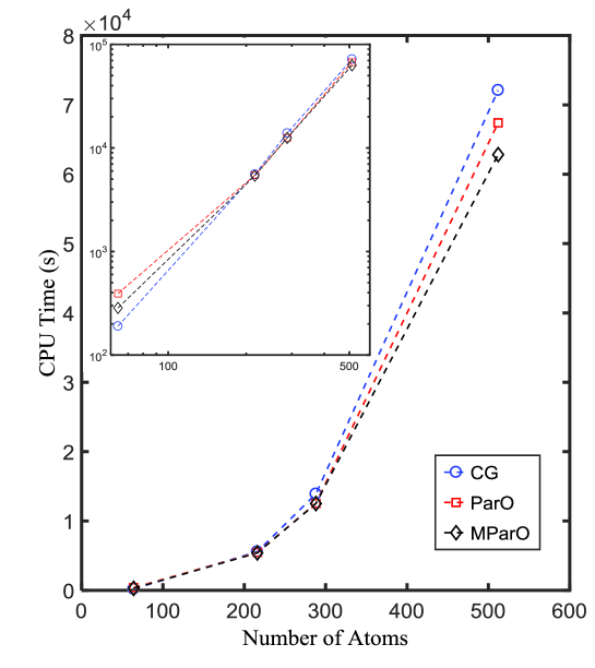
Figure 1: (Color online) CPU time vs the system size (number of atoms) for the MgO crystals for the different methods: CG, ParO, and MParO are reported in blue, red, and black, respectively. The larger the system, the more our algorithms are advantageous in reducing the computational cost.

5.1.2 Aluminium crystals

The second test set consists of two Al crystals of $3\times 3\times 3$ and $4\times 4\times 4$ supercells, hence containing $108$ and $256$ aluminum atoms, respectively. Generally, when dealing with a metal, a dense grid of k points should be used. However, here, we are mainly interested in comparing the behavior of the different methods for the same problem. Therefore, for simplicity, we use only $\Gamma$-point sampling for both systems, and the kinetic-energy cutoff is set to $30Ry$. All results are obtained using one processor.

Table 2 shows the detailed information for Al crystals obtained by the different methods for the default setting where mixing_beta parameter in the Broyden mixing is set to $0.7$. From Table 2 it can be seen that for the smaller system the total energies by both our methods and CG converge. However, for the system which contains $256$ atoms, ParO and MParO converge while CG does not. This can be seen more clearly from Fig.2a, where the SCF error for Al crystal containing $256$ atoms as a function of SCF iteration by the different methods is shown.

$N_{\mathrm{atom}}$	DOFs	Method	$N_{\mathrm{scf}}$	Time (s)	Error of energy
108	13805	CG	16	647	$8\times 10^{-8}$
		ParO	60	1534	$5\times 10^{-8}$
		MParO	17	570	$1\times 10^{-8}$
256	37387	CG	$*$	$*$	$*$
		ParO	46	15917	$5\times 10^{-8}$
		MParO	29	10239	$1\times 10^{-8}$

• $*$ For this case, we can not get the convergent results.

Table 2: Results for Al crystals of different sizes obtained using CG, ParO and MParO with one processor for the default setting where mixing_beta is set to $0.7$. For large system, our methods ParO and MParO can get convergent results while CG can not.

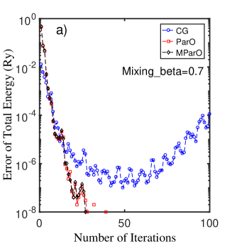
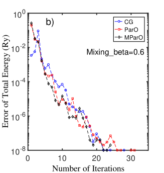
Figure 2: (Color online) The error of total energy vs the number of iterations for Al crystal made of $4\times 4\times 4$ supercell for the different methods for the default setting with different choice of mixing_beta. CG, ParO, and MParO are reported in blue, red, and black, respectively. When mixing_beta is set to $0.7$, ParO and MParO converge while CG does not, but when mixing_beta is set to $0.6$, all the three methods CG, ParO, and MParO converge.

There are many strategies that can be adopted to improve SCF convergence and, for instance, reducing mixing_beta to $0.6$ is enough to make the CG method converge. However our aim here is to compare the different methods in the same conditions. The results for all methods, CG, ParO, and MParO with the modified setting are reported in Table 2 and Fig. 2b where it can be seen that convergence, in terms of number of iterations needed to be achieved, is improved for all methods, and ParO and MParO are competitive with or outperform CG in terms of timing. Of course many more tests would be needed to draw general conclusions about the relative merits of the different methods.

$N_{\mathrm{atom}}$	DOFs	Method	$N_{\mathrm{scf}}$	Time (s)	Error of energy
256	37387	CG	29	14222	$1\times 10^{-8}$
		ParO	33	14580	$3\times 10^{-8}$
		MParO	25	10958	$1\times 10^{-8}$

Table 3: Results for an Al crystal made of $4\times 4\times 4$ supercell obtained using CG, ParO and MParO with one processor for the case of mixing_beta being set to 0.6. All the methods CG, ParO, and MParO converge.

5.2 Good scalability of parallelization

In this subsection, we will use a Si crystal consisting of a $5\times 5\times 5$ supercell with $1000$ silicon atoms as example to show the good parallel scalability of our new algorithms. For this system, the number of computed orbitals is $2000$. The cutoff energies are set to be $45Ry$ and the corresponding Brillouin zones are sampled by only the $\Gamma$-point.

Table 4 show the detailed information for Si crystal by the different methods using $80$, $160$, $320$, $640$ processors, respectively. Fig. 3 shows CPU time for Si crystal as a function of the number of processors for different methods. For the system considered here, it is known that when the number of processors is smaller than $80$, the parallel efficiency of the plane-wave parallelization is relatively high. Therefore, for testing our algorithms with $160$, $320$, $640$ processors, the bands are divided into $2$, $4$, $8$ groups, respectively. For each group, $80$ processors are used for the plane-wave parallelization. For the CG method, since there is no band parallelization, all processors are partitioned using only the plane-wave parallelization.

	CG		ParO			MParO
$N_{\mathrm{procs}}$	$N_{\mathrm{scf}}$	Time(s)	$N_{\mathrm{group}}$	$N_{\mathrm{scf}}$	Time(s)	$N_{\mathrm{group}}$	$N_{\mathrm{scf}}$	Time(s)
80	15	30562	1	46	43220	1	15	27760
160	15	16897	2	46	22647	2	15	14114
320	15	9790	4	46	12299	4	15	8086
640	15	6933	8	46	7620	8	15	4476

Table 4: Results for a Si crystal with $1000$ atoms in the supercell obtained using CG, ParO and MParO with increasing number of processors. The behavior of ParO and MParO is better and better with the increasing of processors, especially for MParO.

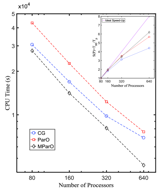
Figure 3: (Color online) CPU time vs the number of processors for a Si crystal with $1000$ atoms in the supercell for the different methods: CG, ParO, and MParO are reported in blue, red, and black, respectively. The inset shows the speed-up obtained as $S(p)=\frac{T_{80}}{T_{p}}$ with $p$ the number of processors used, where $T_{p}$ is the wall time cost by $p$ processors, the purple line is the ideal speed-up $\frac{p}{80}$. The parallel scalability of ParO and MParO is better than that of CG.

From Table 4, it can be seen that the CPU time cost for MParO is shorter than that for CG, while the CPU time cost for ParO is longer than that for CG. However, from Fig. 3 we can see that when the number of processors is larger than $320$, the curves obtained by ParO and MParO are steeper than that obtained by CG. From this it can be seen that the parallel scalability of our new methods is better than CG, especially for MParO. To see it more clearly, one can also see the figure with speed-up in the inset of Fig. 3. Since using $1$ processor can not obtain the converged results for Si crystal with $1000$ atoms supercell due to the limitation of memory, the speed-up here is obtained by comparing the wall time for cases using different number of processors with that for case of using $80$ processors. From the curves shown in Fig. 3, the advantage of our methods in parallel scalability is obvious.

We should point out that, in our current tests, the cutoff energy is set to be a fixed value. If we can start from a small cutoff energy and increase it until the convergence is reached, we can reduce the computational cost further. From this point of view, we believe our new methods will be more competitive than CG.

6 Discussion and conclusion

Motivated by the parallel orbital-updating approach proposed in Ref. [1, 27], we propose some modified parallel orbital-updating methods for the plane-wave discretization of the Kohn-Sham equation in this paper. We show that, by using the two-level parallelization of the orbital-updating approach, the poor parallel scalability of the plane-wave discretization can be largely improved. Indeed our numerical experiments show that the parallel orbital-updating approach based plane-wave method has considerable potential for carrying out large system computation on modern supercomputers.

We should point out that our two-level parallelization only focuses on the solution of the associated eigenvalue problems resulting from the electronic structure calculations. In fact, in the electronic structure calculations, there are some other possibility for parallelization. For example, when using hybrid functionals for approximating the exchange-correlation energy, the exchange potential can be obtained by solving many different Poisson equations, which can be done in parallel intrinsically. Any such kind of parallelization can be combined with our algorithms and hence further increase the parallelization.

As we have pointed out at beginning and at the end of Section 5, the cutoff energy was set to a fixed value in all our tests. To achieve the gradual increase of the cutoff energy, one needs to design some efficient a posteriori error estimator to tell how to evaluate and improve the approximate accuracy based on increasing the cutoff energy. It is indeed our on-going work to design such kind of a posteriori error estimator and then increase the cutoff energy gradually until the accuracy has been reached, which will be addressed elsewhere. We believe that in that case, the parallel efficiency of our new algorithms will become even better.

References

- [1] X. Dai, X. G. Gong, A. Zhou, and J. Zhu, A parallel orbital-updating approach for electronic structure calculations, arXiv:1405.0260 (2014).
- [2] P. Hohenberg and W. Kohn, Inhomogeneous electron gas, Phys, Rev. B, 136 (1964), pp. B864-B871.
- [3] E. Kaxiras, Atomic and Electronic Structure of Solids, Cambridge University Press, Cambridge, UK, 2003.
- [4] W. Kohn and L. J. Sham, Self-consistent equations including exchange and correlation effects, Phys. Rev. A, 140 (1965), pp. 1133-1138.
- [5] R. G. Parr and W. T. Yang, Density-Functional Theory of Atoms and Molecules, Clarendon Press, Oxford, 1994.
- [6] G. Kresse and J. Furthmüller, Efficient iterative schemes for ab initio total-energy calculations using a plane-wave basis set, Phys. Rev. B, 54 (1996), pp. 11169-11186.
- [7] R. Martin, Electronic Structure: Basic Theory and Practical Methods, Cambridge University Press, London, 2004.
- [8] VASP, www.vasp.at.
- [9] Quantum ESPRESSO, www.quantum-espresso.org.
- [10] ABINIT, www.abinit.org.
- [11] E. R. Davidson, The iterative calculation of a few of the lowest eigenvalues and corresponding eigenvectors of large real-symmetric matrices, J. Comput. Phys., 17 (1) (1975), pp. 87-94.
- [12] M. C. Payne, M. P. Teter, D. C. Allan, T. A. Arias, and J. D. Joannopoulos, Iterative minimization techniques for ab initio total-energy calculations: molecular dynamics and conjugate gradients, Rev. Mod. Phys., 64 (1992), pp.1045-1097.
- [13] J. Hutter, H. P. Lüthi, and M. Parrinello, Electronic structure optimization in plane-wave- based density functional calculations by direct inversion in the iterative subspace, Comput. Mater. Sci., 2 (1994), pp. 244-248.
- [14] M. L. Cohen and V. Heine, The fitting of pseudopotentials to experimental data and their subsequent application, Solid State Phys., 24 (1970), pp. 37-248.
- [15] J. C. Phillips, Energy-band interpolation scheme based on a pseudopotential , Phys. Rev., 112 (1958), pp. 685-695.
- [16] D. D. Johnson, Modified Broyden’s method for accelerating convergence in self-consistent calculations, Phys. Rev. B, 38 (1988), pp. 12807-12813.
- [17] P. Pulay, Convergence acceleration of iterative sequences the case of scf iteration, Chem. Phys. Lett., 73 (1980), pp. 393-398.
- [18] P. Pulay, Improved SCF convergence acceleration, J. Comput. Chem., 3 (1982), pp. 556- 560.
- [19] D. Singh, H. Krakauer, and C. S. Wang, Accelerating the convergence of self-consistent linearized augmented-plane-wave calculations, J. Phys. Rev. B, 34 (1986), pp. 8391-8393.
- [20] G. P. Srivastava, Broyden’s method for self-consistent field convergence acceleration, J. Phys. A, 17 (1984), pp. 317-321.
- [21] P. E. Blöchl, Projector augmented-wave method, Phys. Rev., B 50 (1994), pp. 17953-17979.
- [22] P. E. Blöchl, Generalized separable potentials for electronic-structure calculations, Phys. Rev. B, 41 (1990), pp. 5414-5416.
- [23] D. Vanderilt, Soft self-consistent pseudopotentials in a generalized eigenvalue formalism, Phys. Rev. B, 41 (1990), pp. 7892-7895.
- [24] D. R. Hamann, M. Schlüter, and C. Chiang, Norm-conserving pseudopotentials, Phys. Rev. Lett., 43 (1979), pp. 1494-1497.
- [25] N. Troullier and J. L. Martins, Efficient pseudopotentials for plane-wave calculations, Phys. Rev. B, 43 (1991), pp. 1993-2006.
- [26] Quantum ESPRESSO, www.quantum-espresso.org/wp-content/uploads/Doc/INPUTPW.html .
- [27] X. Dai, Z. Liu, X. Zhang, and A. Zhou, A parallel orbital-updating based optimization method for electronic structure calculations, arXiv:1510.07230 (2015).