HIDES spectroscopy of bright detached eclipsing binaries from the Kepler field – II. Double- and triple-lined objects.
Abstract
We present the results of our spectroscopic observations of eight detached eclipsing binaries (DEBs), selected from the Kepler Eclipsing Binary Catalog. Radial velocities (RVs) were calculated from high resolution spectra obtained with the HIDES spectrograph, attached to the 1.88-m telescope of the Okayama Astrophysical Observatory, and were used to characterize the targets in combination with the Kepler light curves. For each binary we obtained a full set of orbital and physical parameters, reaching precision below 3% in masses and radii for 5 pairs. By comparing our results with theoretical models, we assess the distance, age and evolutionary status of the researched objects. We also study eclipse timing variations of selected objects, and identify a new system with a Dor pulsator. Two systems are triples, and show lines coming from three components. In one case the motion of the outer star and the perturbation in the RVs of the inner binary are clearly visible and periodical, which allows us to directly calculate the mass of the third star, and inclination of the outer orbit. In the second case we only see a clear motion of the tertiary, and investigate two scenarios: that it is a linear trend coming from the orbital motion around the inner binary, and that it is caused by a planetary mass companion. When possible, we also compare our results with the literature, and conclude that only by combining photometry with RVs it is possible to obtain correct physical parameters of both components of a DEB.
keywords:
binaries: spectroscopic – binaries: eclipsing – stars: evolution – stars: fundamental parameters – stars: late-type – stars:individual: KIC 06525196, KIC 07821010, KIC 08552540, KIC 09641031, KIC 10031808, KIC 10191056, KIC 10987439, KIC 119227821 Introduction
The field of stellar astrophysics has benefited from the launch of space missions dedicated for precise photometry, like MOST, CoRoT, or Kepler. High-precision light curves (LCs), of a quality not possible to obtain before from the ground, have revolutionized such branches of astrophysics as asteroseismology or eclipsing binaries. The latter are one of the most important objects in astronomy, as they allow for direct determination of parameters like mass and radius, which are very difficult or impossible to obtain with a different method. Such a knowledge is the basis for further studies of, for example, stellar structure and evolution theory, population synthesis, galactic archaeology, cosmic distance scale, extrasolar planets, etc. (Torres et al., 2010). No wonder that for decades researchers were interested in obtaining very precise and accurate basic stellar parameters. It is now believed that the results (e.g. masses and radii) are useful for the purposes of modern astrophysics when they are determined with the precision of 2-3 per cent or better (Lastennet & Valls Gabaud, 2002; Torres et al., 2010; Southworth, 2015). To reach it, one needs high quality spectroscopic and photometric data. The former is usually obtained with stable high-resolution echelle spectrographs, while the source of the most precise photometry was the original Kepler mission.
This paper is a continuation of the research on bright Kepler DEBs, some of which have been described in Hełminiak et al. (2015b) and Hełminiak et al. (2016, hereafter Paper I). The latter work presents the whole observing program in more details. Here we focus on double- and triple-lined systems. Section 2 describes the objects, Section 3 presents the data and methodology, and results are summarised in Section 4, followed by a discussion in Section 5.
2 Targets
| KIC | KOI | Other name | RA (deg) | DEC (deg) | (d)a | (BJD-2450000)a | 3rd?b | ||
|---|---|---|---|---|---|---|---|---|---|
| 06525196 | 5293 | TYC 3143-604-1 | 292.7180 | 41.9225 | 3.420604 | 4954.352139 | 5966 | 10.154 | yes |
| 07821010 | 2938 | TYC 3146-1340-1 | 291.3199 | 43.5955 | 24.238243 | 4969.615845 | 6298 | 10.816 | — |
| 08552540 | 7054 | V2277 Cyg | 288.8904 | 44.6170 | 1.0619343 | 4954.105667 | 5749 | 10.292 | — |
| 09641031 | 7211 | FL Lyr, HD 179890 | 288.0203 | 46.3241 | 2.178154 | 4954.132713 | 5867 | 9.177 | — |
| 10031808 | 7278 | HD 188872 | 298.7976 | 46.9302 | 8.589644 | 4956.430326 | N/Ac | 9.557 | — |
| 10191056 | 5774 | WDS J18555+4713 | 283.8663 | 47.2283 | 2.4274949 | 4955.031469 | 6588 | 10.811 | yes |
| 10987439 | 7396 | TYC 3561-922-1 | 296.8259 | 48.4434 | 10.6745992 | 4971.883920 | 6182 | 10.810 | — |
| 11922782 | 7495 | T-Cyg1-00246 | 296.0074 | 50.2326 | 3.512934 | 4956.247158 | 5581 | 10.460 | — |
a For the eclipsing binary, where is the primary eclipse mid-time;
b ‘yes’ if lines from a third star are seen;
c No temperature given in the KEBC.
For our program we selected targets from the Kepler Eclipsing Binary Catalog (KEBC; Prša et al., 2011; Slawson et al., 2011; Kirk et al., 2016)111http://keplerebs.villanova.edu/. The basic target selection criteria were as follows:
-
1.
Kepler magnitude , to have the targets within the brightness range of the telescope.
-
2.
Morphology parameter (Matijevič et al., 2012) to exclude contact and semi-detached configurations.
-
3.
Effective temperature from K to have only late type systems, with many spectral features. We querried the temperatures from the Kepler Input Catalog (KIC; Kepler Mission Team, 2009).
So far in our program we have observed 21 objects, and published data for 10 of them, and a publication dedicated to one more multiple system is in preparation. In this work we present eight more system that are either double- or triple-lined spectroscopic binaries (SB2 or SB3). They are summarized in Table 1. For each of them we briefly present the basic information below. Unless stated otherwise, the eclipsing nature of a target was discovered by the Kepler mission, and no radial velocity data have been published till date. As all the KEBC eclipsing binaries, they all have their entries in the Kepler Object of Interest (KOI)222http://exoplanetarchive.ipac.caltech.edu/cgi-bin/TblView/nph-tblView?app=ExoTbls&config=koi database since DR24, and most of them are flagged as false positives. The targets, obviously, appear in several catalogue papers related to the Kepler mission (like Coughlin et al., 2011; Tenenbaum et al., 2012; Armstrong et al., 2014).
-
KIC 06525196 = KOI 5293, TYC 3143-604-1: It is a target with periodic eclipse timing variations (ETV; d), identified first by Rappaport et al. (2013), and later by Borkovits et al. (2016). Both groups give the orbital parameters of the outer orbit. Three narrow-line components are visible in the spectra, their RVs can be measured, solutions for both orbits (inner – eclipsing, and outer) can be obtained, and masses of all three stars measured directly.
-
KIC 07821010 = KOI 2938, TYC 3146-1340-1: This system has the longest orbital period in our sample, and a significant eccentricity. It probably hosts a non-transiting, circumbinary planet, which was first announced in a conference presentation by W. Welsh333http://www.astro.up.pt/investigacao/conferencias/
/toe2014/files/wwelsh.pdf but the proper publication is still to be announced (Fabrycky et al., in prep.). Borkovits et al. (2016) confirmed such possibility, by finding periodic modulations of the ETVs. Till now, absolute stellar parameters have also been presented on a conference only, first by Sharp et al. (2014). Our observations started independently and simultaneously, without prior knowledge of the work by Fabrycky et al., and our study utilizes only our HIDES data. -
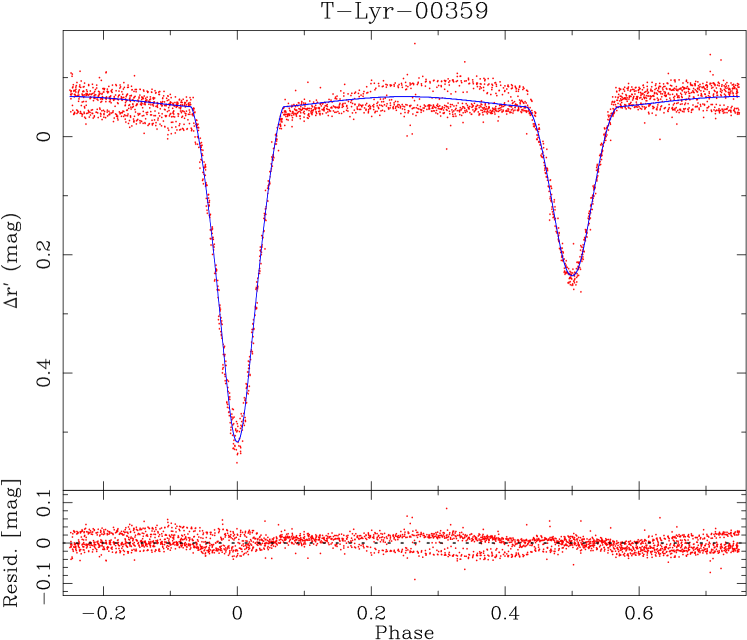
KIC 08552540 = KOI 7054, V2277 Cyg, T-Lyr1-00359, ASAS J191534+4437.0, BD+44 3087: This star is classified in KOI database as a planetary candidate (PC) despite being an eclipsing binary known before the Kepler launch. Discovered and first identified as a DEB by the Robotic Optical Transient Search Experiment 1 (ROTSE1; Akerlof et al., 2000), first reported by Diethel (2001). Later also observed by the Trans-atlantic Exoplanet Survey (TrES; Alonso et al., 2004), and listed in the catalogue of variable stars in the Kepler field of view of the All Sky Automated Survey (ASAS-K; Pigulski et al., 2009). By analysing the TrES light curve only, Devor et al. (2008) estimated the masses of both components: 1.655(15) and 1.296(13) M⊙ for the primary and secondary, respectively. Our spectroscopy allows us to revise these values. Several authors report ETVs (Gies et al., 2012, 2015; Conroy et al., 2014), but attribute them to the evolution of spots on the surface of both components.
-
KIC 09641031 = KOI 7211, FL Lyr, HD 179890, HIP 94335: This is the only system in our sample with the full physical solution known before the Kepler satellite was launched. Identified as eclipsing by Morgenroth (1935) and as (single-lined) spectroscopic by Struve et al. (1950). The most complete analysis so far was done by Popper et al. (1986), who give 1.218(16) M⊙, 1.283(30) R⊙ for the primary, and 0.958(11) M⊙, 0.963(30) R⊙ for the secondary. Recently, Kozyreva et al. (2015) presented their own ETVs and claimed a discovery of a planetary-mass circumbinary companion candidate. They gave three possible solutions, based on different orbital periods of the inner binary and the outer body. In each case the time span of Kepler data was shorter than the circumbinary period, therefore all solutions are only preliminary and uncertain.
-
KIC 10031808 = KOI 7278, HD 188872: The only star from our sample that has no given in the KEBC, but a value of 6331 K can be found in the KOI database. Except brightness and position measurements, no literature data are available.
-
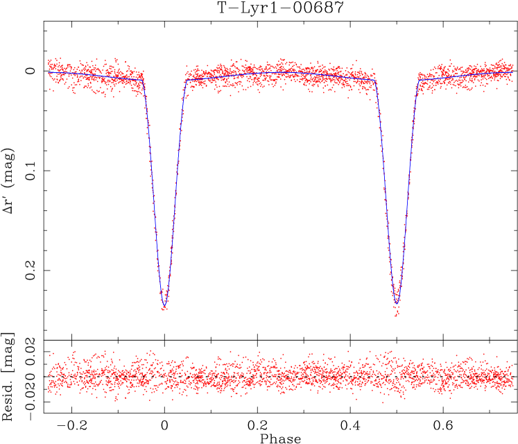
KIC 10191056 = KOI 5774, WDS J18555+4713, T-Lyr1-00687, ASAS J185528+4713.7, BD+47 2717: Another star classified in the KOI database as PC, despite being known to be an eclipsing binary. This is another triple-lined system in our sample. Reported by Couteau (1983) as a visual binary, with components of magnitudes 10.97 and 14.80, separated in 1982 by 1.16 arcsec. Re-observed only recently by Ziegler et al. (2017), who give the separation of 1.32 arcsec, and at 6000 Å (from Robo-AO) and in band (from Gemini-N/NIRI). Identified for the first time as an eclipsing binary by the TrES survey, and later by ASAS-K. By analysing the TrES light curve only, Devor et al. (2008) estimated the masses of both components: 1.209(13) and 1.208(13) M⊙ for the primary and secondary, respectively. Our spectroscopy allows us to revise these values. In our spectra we see two sets of wider lines, belonging to the components of the eclipsing pair, and another, narrow set coming from a third star. This system also has ETVs reported by several authors (Gies et al., 2012, 2015; Conroy et al., 2014), but no secure conclusions were drawn.
-
KIC 10987439 = KOI 7396, TYC 3561-922-1: This system has the second longest period in our sample, and the narrowest spectral lines. Except brightness and position measurements, no literature data are available.
-
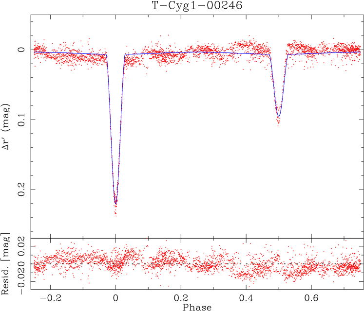
KIC 11922782 = KOI 7495, T-Cyg1-00246, TYC 3565-643-1: This system was first observed by the TrES survey and identified as a detached eclipsing binary by Devor et al. (2008). By analysing the light curve only they estimated the masses of both components: 1.498(26) and 0.970(32) M⊙ for the primary and secondary, respectively. Our spectroscopy allows us to revise these values.
3 Data and analysis
Most of the methods and sources of data used in this work are identical to those from Paper I, and please refer to it for a detailed description. Here we only describe them briefly, and focus more on those that were not used in Paper I due to a different nature of the researched objects.
3.1 HIDES observations and RV measurements
The spectroscopic observations were carried out during several runs between July 2014 and October 2016, at the 1.88-m telescope of the Okayama Astrophysical Observatory (OAO) with the HIgh-Dispersion Echelle Spectrograph (HIDES; Izumiura, 1999). The instrument was fed through a circular fibre, for which the light is collected via a circular aperture of projected on-sky diameter of 2.7 seconds of arc, drilled in a flat mirror that is used for guiding (Kambe et al., 2013). An image slicer is used in order to reach both high resolution () and good efficiency of the system. Spectra extraction was done under iraf, using procedures dedicated to HIDES. Wavelength solution was based on ThAr exposures taken every 1-2 hours, which allows for stability of the order of 40 m s-1. The resulting spectra span from 4360 to 7535 Å.
For the radial velocity measurements we used our own implementation of the todcor technique (Zucker & Mazeh, 1994), which finds velocities of two stars and simultaneously. As templates we used synthetic spectra computed with ATLAS9 and ATLAS12 codes (Kurucz, 1992). Single measurement errors were calculated with a bootstrap approach (Hełminiak et al., 2012), and used for weighting the measurements during the orbital fit, as they are sensitive to the signal-to-noise ratio () of the spectra and rotational broadening of the lines.
The todcor is optimized for double-lined spectroscopic binaries, but our sample includes triple-lined objects. For those, the velocities of the eclipsing pair were found from the global maximum, as each of these components contribute more to the total flux than the third star. The tertiary’s velocities were found from a local maximum, where was for the tertiary, and for the primary of the eclipsing pair.
In case of a hierarchical triple, for which we see motion of all components, the outer orbits can also be modelled, or at least the mass ratio (tertiary to the inner binary) can be calculated (when the outer period is unknown). For this, we use the measured velocities of the third star, denoted as B, and variations of the systemic velocity of the inner pair A (Aa+Ab). In general, the two RVs of a spectroscopic binary – – measured at any time , are related by:
| (1) |
(Wilson, 1941) where and are the systemic velocity and mass ratio (secondary over primary), respectively. Without a direct interaction between two stars, remains constant, but can change in time, if the binary is orbited by another body. Assuming we can write:
| (2) |
We used this formula to calculate of the Aa+Ab pair at a given moment of observation , and used these values in the orbital analysis of the A+B outer orbit. The values of were taken from the solution of the inner orbit.
All radial velocity measurements obtained from our HIDES spectra, together with their errors and of the spectra, are listed in Table 8 in the Appendix. For the triples KIC 06525196 and 10191056 we also list the velocities of the third star, and measurements of for each observation (in the column ‘’).
3.2 Publicly available data
Other data used in this study are publicly available. The long cadence Kepler photometry for all targets is available for download from the KEBC. It was the main source of the photometry used in this work. We used the de-trended relative flux measurements , that were later transformed into magnitude difference , and finally the catalogue value of was added. Short cadence data, available for some of the targets, were not used due to their large amount and computer time required to analyse them.
Additional TrES data for KIC 08552540, 10191056, and 11922782 can be found in the on-line catalogue of eclipsing binaries identified by Devor et al. (2008)444http://vizier.u-strasbg.fr/viz-bin/VizieR-3?-source=J/AJ/135/850/table7, who used the LCs and information about total observed colours of a binary (but no spectroscopy) to directly determine the absolute masses and ages of those systems. We include them in our work in order to directly compare TrES and Kepler curves, and our results with those from Devor et al. (2008).
Two systems have and -band LCs available from the ASAS-K website555http://www.astrouw.edu.pl/asas/i_kepler/kepler_tab.html. These are KIC 08552540 = ASAS J191534+4437.0 and KIC 10191056 = ASAS J185528+4713.7. The quality of data is rather poor, and the LCs do not contain many points, so the eclipses are not always sampled properly. Nevertheless, we made an attempt to use them to asses the observed colours of each component, therefore having independent estimates of temperatures.
Finally, we’d like to note that all systems have their LCs publicly available from the
SuperWASP archive666http://exoplanetarchive.ipac.caltech.edu/cgi-bin/TblSearch/nph-tblSearchInit?app=ExoTbls&config
=superwasptimeseries.
We have, however, decided not to analyse them. The photometric precision of
Kepler is much better, these LCs were not used to determine absolute physical parameters,
and, themselves, they do not contain any important information
that would not be possible to obtain from other data, like colours.
Archival RV measurements can be found for KIC 09641031 (FL Lyr) in several literature sources, with the most recent RV curve published by Popper et al. (1986). Before that, this system was studied by Struve et al. (1950), but velocities of only one component were given. We did not include the literature RVs in our study, and there is not much improvement when they are combined with our more accurate HIDES measurements.
3.3 Eclipse timing variations
Four systems from our sample – KIC 06525196, 07821010, 09641031, and 10191056 – have been reported in at least one study to show eclipse timing variations (ETVs). These are differences between the observed and predicted moments of eclipses, which may be caused by a phenomenon intrinsic to the system (like spot evolution, apsidal motion), or by a third body orbiting the eclipsing pair.
Because not all authors publish their ETVs, and because the measured ETVs can differ, depending on the method that was used, we decided to calculate our own. As in Paper I, we used the radio-pulsar-style method from Kozłowski et al. (2011). In this method, a template LC is created by fitting a trigonometric (harmonic) series to a complete set of photometric data. Then, the whole set of photometric data is divided to a number of subsets. Their number is arbitrary, but for this study we set it to 200. For each subset, the phase/time shift is found by fitting the template curve with a least-squares method. In the final stage we removed the obvious outliers, less than 10 in each case.
We have calculated the ETVs for three systems: KIC 06525196, 09641031, and 10191056. We omitted KIC 07821010 because of the ongoing analysis by Fabrycky et al. (in prep.). Our ETVs are given in Table 9 in the Appendix.
3.4 Orbital solutions
The orbital solutions were found using our own procedure called v2fit (Konacki et al., 2010). It is capable of working in different modes, and including various optional effects (e.g. relativistic or tidal), but we used it mainly in the simplest mode, where a double-Keplerian orbit is fit to a set of RV measurements of two components, utilizing the Levenberg-Marquardt minimization scheme. The fitted parameters are: orbital period , zero-phase 777Defined as the moment of passing the pericentre for eccentric orbits or quadrature for circular., systemic velocity , velocity semi-amplitudes , eccentricity and periastron longitude , although in the final runs the last two parameters were usually kept fixed on values found by jktebop fit (Sect. 3.5). Depending on the case, we also included such effects as: the difference between systemic velocities of two components, , linear and quadratic trends in , and periodic modulations of the inner binary’d , interpreted as influence of a circumbinary body on an outer orbit, parametrized analogously by orbital parameters , , , , and . In such case is defined in the code as the systemic velocity of the whole triple. Whenever applicable, we simplified our fit by keeping the orbital period on the value given in the KEBC. Also, we were first letting to be fit for, but when the resulting value was indifferent from zero, we were keeping it fixed.
Formal parameter errors of the fit are estimated by forcing the final reduced to be close to 1, either by multiplying them by a certain factor, or adding in quadrature a systematic term (jitter). Because the code weights the measurements on the basis of their own errors, which are sensitive to and , we mainly used the first option in our analysis. The exception are active stars that clearly show spot-originated brightness variations. For these, the jitter compensates for the additional RV scatter introduced by the spots. The errors given in Table 8 are the multiplied ones, for which .
Systematics that come from fixing a certain parameter in the fit are assessed by a Monte-Carlo procedure, and other possible systematics (like coming from poor sampling, low number of measurements, pulsations, etc.) by a bootstrap analysis. All the uncertainties of orbital parameters given in this work already include the systematics.
3.5 Light curve solutions and absolute parameters
For the light curve analysis of Kepler and TrES data we used version 28 (v28) of the code jktebop (Southworth et al., 2004a, b), which is based on the ebop program (Popper & Etzel, 1981). As described in Paper I, the best fit was found on the complete Q0-Q17 Kepler light curve, but errors were estimated with a residual-shift (RS) method (Southworth et al., 2011), run on data from each quarter separately. This approach is several times faster than running RS on the complete curve, and properly includes the influence of such systematic effects as spots or pulsations, which we effectively treat as red (correlated) noise.
On the basis of spectroscopic data we first found the mass ratio , as well as starting values of eccentricity and periastron longitude . We fitted for the period , mid-time of the primary (deeper) minimum , sum of the fractional radii (where ), their ratio , inclination , surface brightness ratio , maximum brightness , third light contribution , as well as for and (their final values are from the jktebop runs, unless stated otherwise).
An initial model was done to roughly estimate the radii and masses (to obtain ) and then the temperatures from the PAdova and TRieste Stellar Evolution Code (PARSEC; Bressan et al., 2012)888http://stev.oapd.inaf.it/cgi-bin/cmd isochrones. These results were used to estimate the limb darkening (LD) coefficients, that were held fixed during the major fit, but perturbed during the RS stage. We used the logarithmic limb darkening law (Klinglesmith & Sobieski, 1970), with the coefficients interpolated from the tables published on the PHOEBE website999http://phoebe-project.org/1.0/?q=node/110. We found that results do not change significantly if we put LD coefficients predicted for temperatures and gravities different by 150 K and 0.5 dex. We also tried to set the LD free, but ended up in physically impossible values. The gravity darkening coefficients were always kept fixed at the values appropriate for stars with convective envelopes ().
The results of LC and RV solutions were later combined in order to calculate the absolute values of stellar parameters using the jktabsdim code, available together with the jktebop. As an input, this simple procedure takes orbital period, eccentricity, fractional radii, velocity semi-amplitudes and inclination (all with uncertainties), and returns absolute values of masses and radii (in solar units), and rotational velocities, assuming tidal locking and synchronization. It can also calculate distance to an object, taking effective temperatures of two components, and apparent magnitudes. The jktabsdim does not work on brightnesses in Kepler band, so, unless stated otherwise, for the distance estimation we used and -band entries from Simbad (Wenger et al., 2000). As the final value of distance we adopt a weighted average of five values, calculated for each band from the surface brightness- relations of Kervella et al. (2004). For the majority of distance calculations, we used temperatures found from isochrone fitting (Sect. 3.6 and 5.2). The ones found in KEBC correspond to the total system’s light, and, especially in the case of triples, should not be taken as temperatures of the components.
The problem is easier to solve when independent estimates are known, like in the case of KIC 09461031 = FL Lyr (Popper et al., 1986), or when multi-band light curves are available, so the components’ individual colours can be estimated, like for the two systems with ASAS-K data. In these two cases, the jktebop fits were done to the and -band data mainly to assess the fractional fluxes of each of the components, from which we inferred their observed magnitudes in both bands, and colours. Most of the parameters (like sum and ratio of radii, inclination, ephemerides) were therefore held fixed to values found for Kepler data, and only surface brightness ratio, maximum brightness and third light were fitted for. The uncertainties were calculated with a Monte-Carlo procedure.
We would also like to point out that, in principle, SuperWASPKepler colours are possible to obtain, but both filters are wide and cover similar range of wavelength (400–900 and 400–700 nm for Kepler and SuperWASP, respectively), therefore such colours would not carry much information.
3.6 Comparison with isochrones and age estimation
We use our mass and radius estimations to assess the age and evolutionary status of each system. We compare them with the PARSEC isochrones, which include values of absolute magnitudes in the Kepler band. The isochrones were calculated for ages /yr) of 6.6 to 10.10, every . In few cases the best match is obtained for not being a node of this grid of ages, like . In such situations we generate a separate isochrone for the desired .
For all systems we assume solar metallicity ( in this set), because we lack or estimates that we find reliable. Those from, for example, KIC or MAST are calculated as for single stars, and usually base on photometry only. We do not always find an isochrone that agrees with our results at 1 level, but in no case the agreement is worse than 3. In cases when two significantly different solutions are possible (i.e. resulting in main-sequence or pre-main-sequence stage), we also checked which one better reproduces the resulting flux ratio (from absolute magnitude difference). In all such cases the main-sequence solution turned out to be the preferable one.
From the isochrones we determine the effective temperatures of components. We take the ’s from the isochrone that matches both stars best. For the uncertainty, we take the difference between temperatures predicted by the isochrone matched to the whole system and the one that matches only the particular component, rounded up to 50 K, which we believe is a reasonable precision. If the difference is small, i.e. K, we assume 100 K as a conservative temperature error. We also give all ’s with 50 K precision. These temperatures are later used for distance determination with jktabsdim. Because the true information about the metallicity is missing, the resulting ages should be treated as preliminary, but the evolutionary stages should be reliable.
| KIC | 06525196 Aa | 07821010 | 08552540b | 09641031 | 10031808 | 10191056 Aab | 10987439 | 11922782b |
|---|---|---|---|---|---|---|---|---|
| (d) | 3.42059774(14) | 24.238235(4) | 1.06193441(4) | 2.17815425(7) | 8.5896432(13) | 2.427494881(19) | 10.67459809(33) | 3.5129340(3) |
| (JD-2454900)c | 54.353595(29) | 69.61678(13) | 54.105945(27) | 54.133349(3) | 56.43099(10) | 55.031699(5) | 71.885044(32) | 56.24790(7) |
| (JD-2454900)d | 53.508(12) | 69.313(35) | 53.846(23) | 53.5886(11) | 56.475(74) | 53.931(18) | 60.136(72) | 51.856(20) |
| (km s-1) | 85.96(12) | 66.64(34) | 121.0(1.6) | 93.23(12) | 83.08(28) | 107.0(1.3) | 76.39(10) | 76.04(29) |
| (km s-1) | 91.62(22) | 69.75(32) | 145.9(2.0) | 118.19(30) | 80.42(15) | 119.3(1.0) | 53.00(9) | 97.01(42) |
| (km s-1) | (var) | -17.18(9) | -14.1(1.1) | -37.45(9) | 12.96(17) | (var) | -19.11(11) | -41.84(13) |
| (km s-1) | 0.0(fix) | 0.0(fix) | 0.0(fix) | 0.0(fix) | -0.17(21) | 0.0(fix) | -0.37(19) | 0.0(fix) |
| 0.9383(26) | 0.9554(66) | 0.829(16) | 0.7888(22) | 1.033(4) | 0.897(13) | 1.4413(31) | 0.784(4) | |
| (M⊙) | 1.0240(52) | 1.289(15) | 1.144(36) | 1.1923(66) | 1.705(9) | 1.536(31) | 0.9776(34) | 1.057(10) |
| (M⊙) | 0.9607(36) | 1.231(15) | 0.948(28) | 0.9405(35) | 1.762(13) | 1.378(35) | 1.4090(45) | 0.829(6) |
| (R⊙) | 12.010(17) | 47.98(18) | 5.604(54) | 9.105(14) | 26.723(54) | 10.861(78) | 27.272(28) | 12.019(32) |
| 0.0(fix) | 0.6791(14) | 0.0(fix) | 0.0(fix) | 0.2717(14) | 0.00283(23) | 0.0509(14) | 0.0(fix) | |
| (∘) | — | 58.86(13) | — | — | 94.067(70) | 287.3(1.5) | 51.7(2.3) | — |
| 0.0874(85) | 0.027852(114) | 0.2509(31) | 0.1389(25) | 0.09628(71) | 0.1784(20) | 0.03409(54) | 0.1245(47) | |
| 0.0877(85) | 0.024383(57) | 0.1806(40) | 0.0995(26) | 0.11250(47) | 0.1571(25) | 0.05527(11) | 0.0704(52) | |
| (∘) | 85.15(34) | 89.597(20) | 85.83(46) | 85.36(71) | 83.323(47) | 81.345(75) | 85.614(66) | 85.52(60) |
| 0.906(47) | 0.857(21) | 0.67(14) | 0.434(49) | 0.903(34) | 0.9547(56) | 2.56(22) | 0.46(11) | |
| 0.91(22) | 0.726(13) | 0.292(10) | 0.224(35) | 1.2303(23) | 0.754(43) | 6.48(1.14) | 0.15(3) | |
| 0.243(9) | 0.0(fix) | 0.0(fix) | 0.0(fix) | 0.0(fix) | 0.1866(38) | 0.0(fix) | 0.0(fix) | |
| (M⊙) | 1.0351(55) | 1.289(15) | 1.153(36) | 1.2041(76) | 1.741(9) | 1.590(32) | 0.9862(34) | 1.067(10) |
| (M⊙) | 0.9712(39) | 1.231(15) | 0.956(28) | 0.9498(46) | 1.798(13) | 1.427(36) | 1.4215(45) | 0.836(6) |
| (R⊙) | 1.116(103) | 1.3363(75) | 1.410(22) | 1.269(23) | 2.590(20) | 1.960(26) | 0.932(15) | 1.501(57) |
| (R⊙) | 1.057(103) | 1.1698(52) | 1.015(24) | 0.908(24) | 3.027(14) | 1.726(30) | 1.512(31) | 0.849(63) |
| (R⊙) | 12.053(18) | 47.98(18) | 5.619(54) | 9.135(17) | 26.905(54) | 10.986(80) | 27.352(29) | 12.056(34) |
| 4.358(80) | 4.297(4) | 4.202(12) | 4.312(16) | 3.852(6) | 4.055(10) | 4.493(14) | 4.114(33) | |
| 4.377(85) | 4.392(3) | 4.406(20) | 4.499(23) | 3.731(4) | 4.119(15) | 4.232(18) | 4.503(64) | |
| (km s-1) | 0.26 | 0.15 | 3.02 | 0.42 | 0.50 | 2.50 | 0.129 | 0.37 |
| (km s-1) | 0.41 | 0.48 | 5.26 | 0.71 | 0.30 | 2.28 | 0.042 | 1.02 |
| (mmag) | 2.65 | 0.50 | 12.74 | 5.44 | 1.22 | 0.41 | 0.072 | 8.06 |
a With RVs corrected for the motion around the common centre of mass with star B.
b From jktebop solutions for Kepler curve only.
c Mid-time of the primary (deeper) eclipse.
d Time of pericentre or quadrature.
4 Results
4.1 Double-lined binaries
In this Section we present the results of our analysis of eight double-lined spectroscopic and eclipsing binaries. Their orbital and physical parameters are summarised in Table 2. Presented uncertainties (1) include systematics, estimated with the MC+bootstrap (in v2fit) and residual-shift (in v2fit) methods. We follow the convention that the primary star is the one eclipsed during the deeper minimum, which for circular orbits means the hotter component. The orbital period was taken from the initial jktebop run, and held fixed during the orbital fit. The model radial velocity and light curves are phase-folded with the period of eclipses found in jktebop and with zero-phase set to the primary eclipse mid-time .
4.1.1 KIC 06525196 A
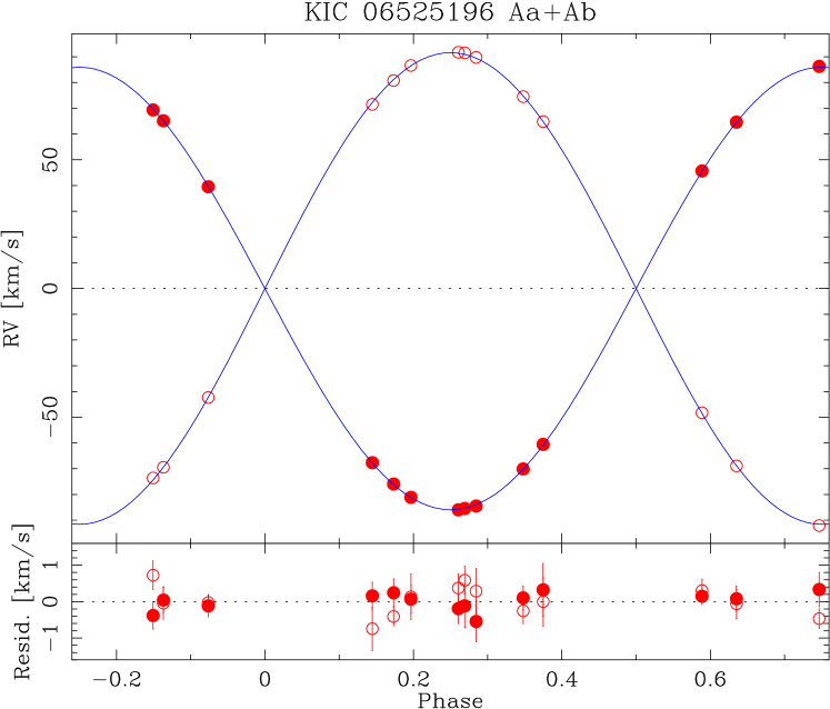
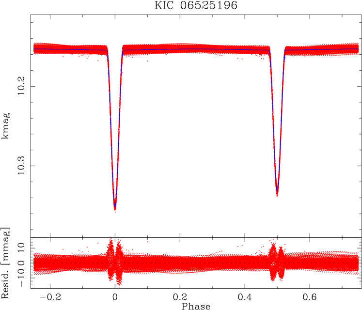
This is one of the two special cases of a triple-lined system in our sample, where three sets of lines are visible. In this hierarchical system the outer orbital period is relatively short (418 d), and we covered it whole with our HIDES observations (time span of 676 d). We use the convention that the inner pair is Aa+Ab, while the outer companion is B. Here we focus only on the Aa+Ab eclipsing pair, leaving the outer orbit of AB for discussion in a further Section.
We have observed this system 14 times with HIDES. Relatively narrow spectral lines allow for quite precise RV measurements. In our orbital model we fitted the parameter of the Aa+Ab orbit, and also for the periodic perturbation coming from the third star. We assumed that both the orbit of the inner pair and the perturbation are Keplerian. We found no evidence for a non-zero eccentricity of the inner pair, nor for a difference in systemic velocities of its components. We reached a very good precision of 0.5–0.4 per cent in masses, but a relatively poor one in radii: 9.2–9.7 per cent. This is mainly caused by the influence of the third body: its contribution to the total flux, but also variations in the shape of eclipses of the phase-folded light curve, coming from the fact that the moment of eclipses varies. This is clearly seen on the complete Q0-Q17 LC, shown in Figure 1 – note the shape of the residuals around eclipses (phases 0.0 and 0.5). One can also note an out-of-eclipse variation, which we interpret as coming from spots that evolve in time. They also hamper the photometric solution. In Fig.1 we also show the RV curves of the inner binary, phase folded with its period and corrected for the influence of the third body. The complete set of orbital and physical parameters is given in Table 2.
4.1.2 KIC 07821010

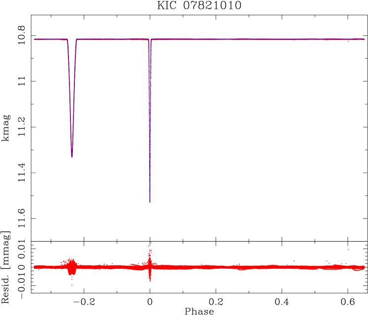
This star is the most eccentric and faintest SB2 in our sample, and the quality of HIDES data was highly dependent on weather conditions. Nine spectra were taken, but four of them are of lower , which can be distinguished by the RV measurement errors, and they hamper the quality of the orbital fit. On the other hand the out-of-eclipse photometric variability is relatively low, so the LC-based parameters were found with very good precision.
The observations and model RV and light curves are presented in Figure 2. The strong deviations from the LC model seen around eclipses are possibly caused by a mismatch in LD coefficients. They also change from quarter to quarter, which can be explained by the presence of the circumbinary planet postulated by Fabrycky et al. As for other systems, we failed to find the LD coefficients when they were set as free parameters during the fit, but they were perturbed during the RS stage, so their influence on resulting parameters is accounted for (mainly on , and ). In the end, we reached a good precision of 1.6 per cent in masses, and 0.7–0.9 per cent precision in radii. It is sufficient for reliable testing of evolutionary models (Lastennet & Valls Gabaud, 2002).
Our value of ratio of the radii is not in a very good agreement with results from Armstrong et al. (2014), who found . Their method bases on the total system’s brightness measurements in several filters, and for this object produced large uncertainties. We thus concluded that their results should be treated with a lot of caution, and decided not to compare our results with theirs for other systems.
4.1.3 KIC 08552540 (V2277 Cyg)
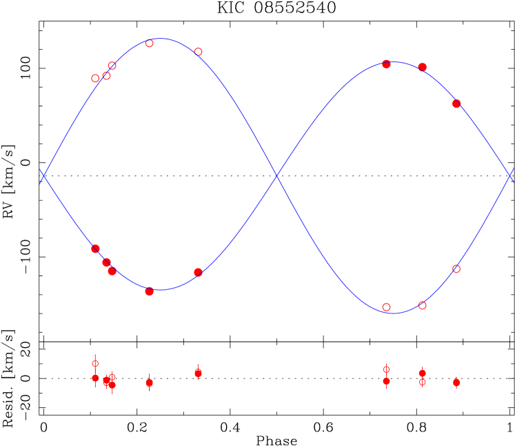
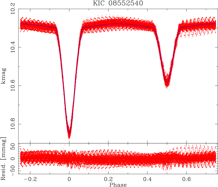
This system has the shortest orbital period in our sample. In our eight HIDES spectra we see that the lines of both components are very broad, suggesting tidal locking and synchronous rotation. This clearly affected the quality of the RV fit. Also, as seen in many late-type, short-period binaries, there is a strong out-of-eclipse brightness modulation that affected the LC modelling. From its character (sine-like shape, evolution in time, variation of brightness in the minima) we conclude that it is caused by the presence of cold spots on both components. Model curves and observations are shown in Fig. 3, and parameters are listed in Table 2. Despite large -es of both RV and light curves, the resulting uncertainties in masses and radii are quite low: 2.9-3.1 and 1.6-2.4 per cent, respectively.
It is worth to note that large spots on solar-mass components of short-period eclipsing binaries are not surprising, and were observed in other systems (e.g. CV Boo: 1.032+0.968 M⊙, d; Torres et al., 2008). They are a result of a presence of magnetic fields stronger than in single stars, enhanced by fast rotation in tidally-locked pairs. Such a situation is common among lower-mass short-period systems. In order to confirm the chromospheric activity, we examined the Hα lines in our spectra, but found no obvious emission features, although the is not always optimal, and the primary’s absorption line may be partially filled. As explained in Paper I, the Ca II H and K lines are not in the HIDES wavelength range.
4.1.4 KIC 09641031 (FL Lyr)
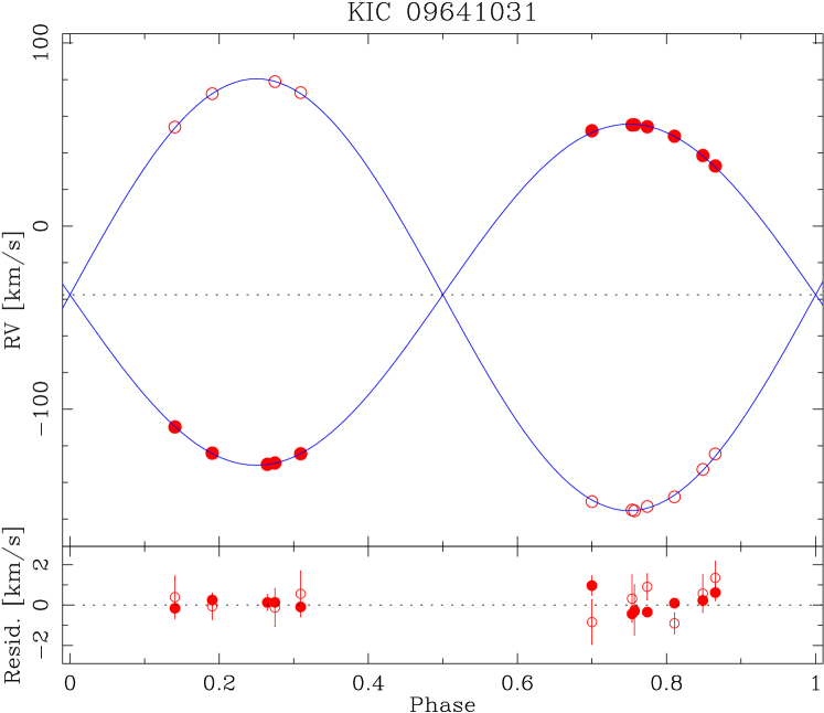
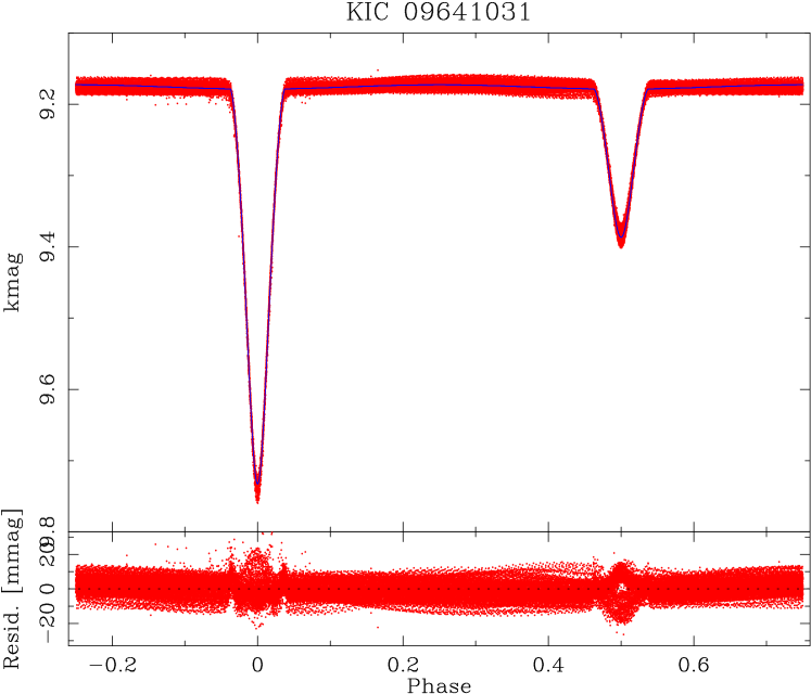
This is the only system from our sample with RV measurements and full physical solution known before the Kepler mission (Popper et al., 1986). It is also among the best-measured systems, that are listed in the on-line DEBCat101010http://www.astro.keele.ac.uk/jkt/debcat/ catalogue (Southworth, 2015). We have acquired twelve HIDES spectra, which is almost two times fewer than in Popper et al. (1986), but the RV precision is significantly better. We have reached a very low uncertainty of 0.48-0.63 per cent in masses, which is 2-2.5 times better than previously. Our precision in radii is also good, and reaches 1.8-2.6 per cent, yet, surprisingly, it is only slightly improved in comparison with Popper et al. (1986), despite superior photometric data. The explanation is, mainly, the influence of spots, clearly visible in Kepler data, and slowly evolving in time. Our uncertainty in fractional radii comes in this case mainly from the spread of RS stage results for each separate quarter. Over the whole course of Kepler observations the brightness modulation averages out in the LC, but for each quarter is slightly different. It is worth to note that the spread of the Kepler residuals is comparable to the spread shown by Popper et al..
| This work | Popper et al. | |
|---|---|---|
| Parameter | (Table 2) | (1986) |
| (d) | 2.17815425(7) | 2.1781542(3) |
| (km s-1) | 93.23(12) | 93.5(5) |
| (km s-1) | 118.19(30) | 118.9(7) |
| 0.1389(25) | 0.140(3) | |
| 0.0995(27) | 0.105(3)a | |
| (∘) | 85.36(71) | 86.3(4) |
| (M⊙) | 1.2041(76) | 1.218(16) |
| (M⊙) | 0.9498(46) | 0.958(11) |
| (M⊙) | 1.269(23) | 1.283(30) |
| (M⊙) | 0.908(24) | 0.963(30) |
aCalculated from the uncertainty of given in Table 17 of Popper et al. (1986), which does not include all sources of errors. When calculated from the fractional radius , and ratio of radii (as in their Table 9), it becomes 0.007.
Our model is presented in Figure 4, with parameters in Table 2. They are compared with the solution by Popper et al. (1986) in Table 3. One can see that we have improved the mass determination for this important system. Other parameters agree very well, with the exception of and , for which our model gives values lower than in Popper et al., at the edge of 1 agreement. This seemingly worse consistency is likely due to the fact that Popper et al. gave their uncertainty of absolute radii of the secondary underestimated (see the comment under their Table 17). This is another reason why our results seem to be only slightly better. They also do not directly give the value (nor the error) of the fractional secondary radius. In Table 9, they only give the fractional primary radius , and the adopted ratio of radii . When the fractional secondary radius and its uncertainty are calculated from these values, with the proper error propagation, we obtain . Our value of is therefore well within their error.
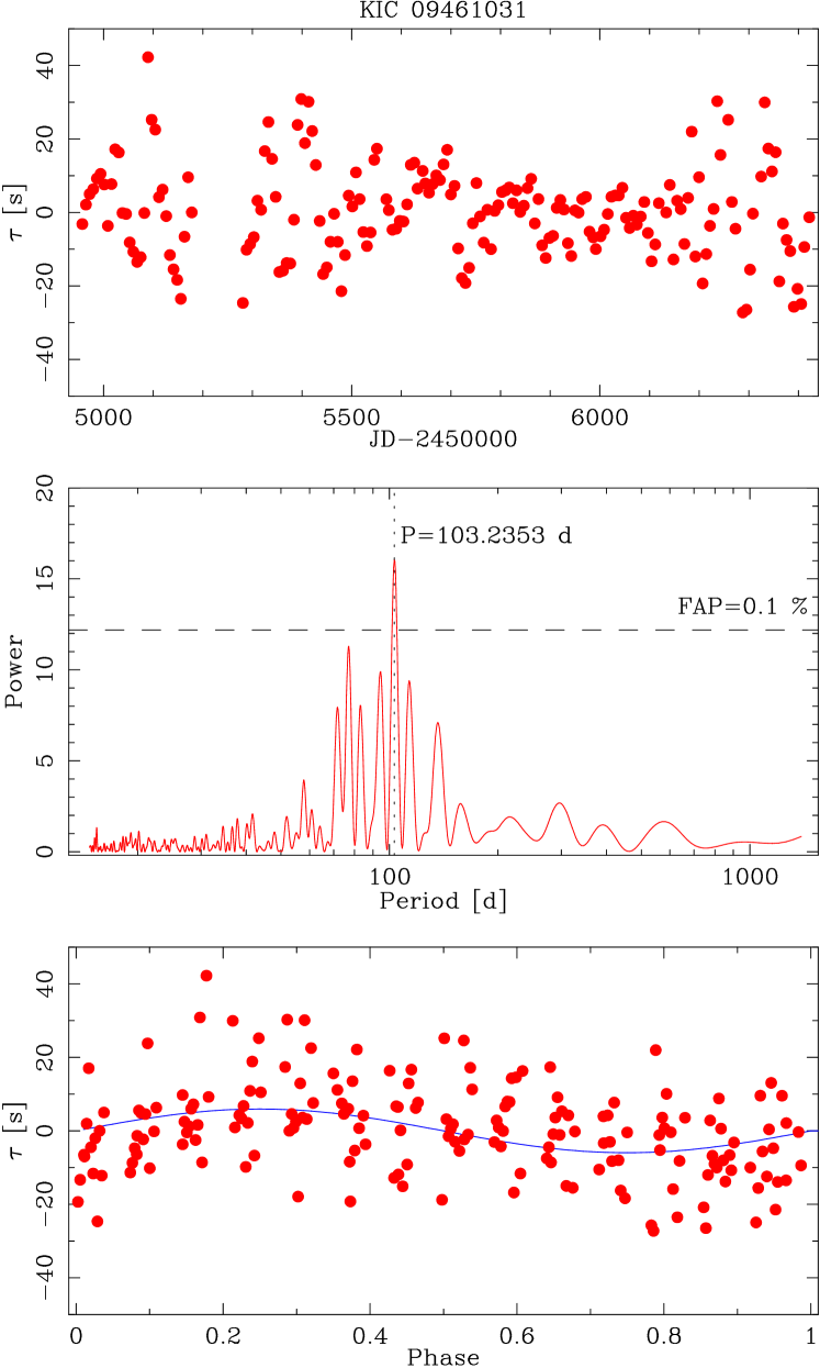
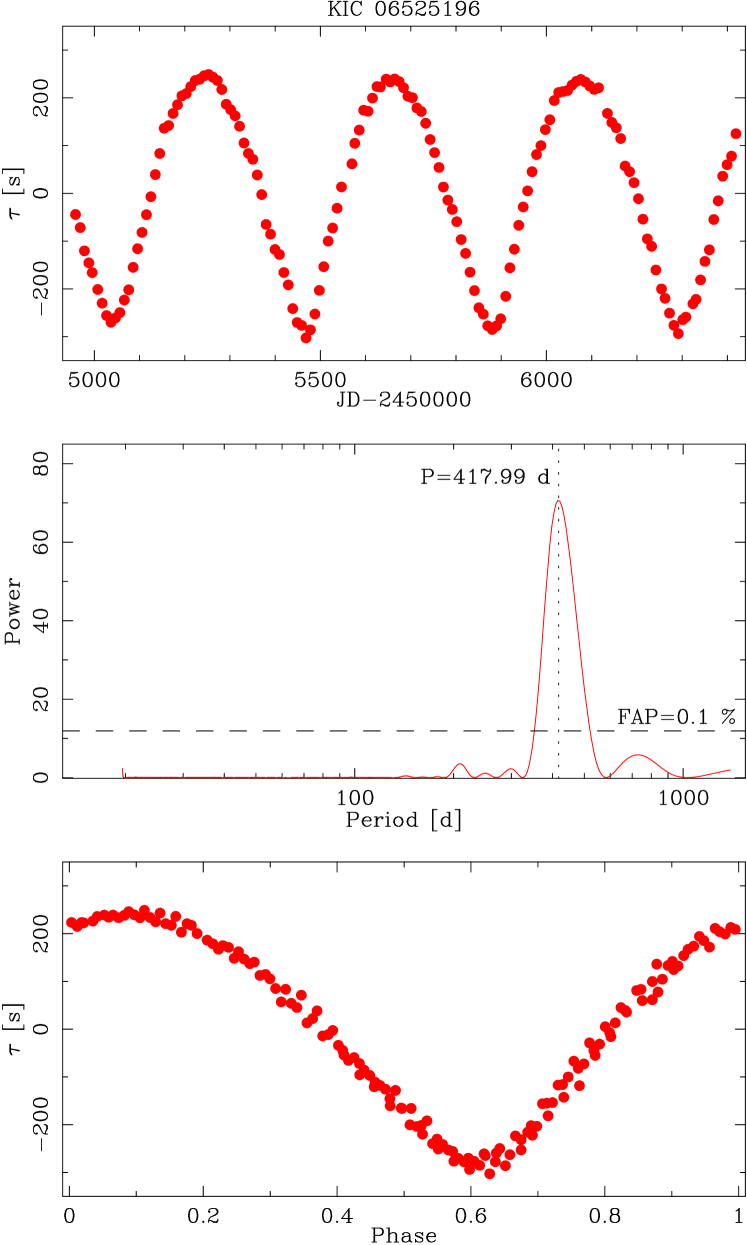
Finally, we examine the claim of Kozyreva et al. (2015) of detectable timing variations,
which they interpret as being caused by a third body on a long-period orbit.
In the Figure 5 we present our own ETVs (),
calculated in a way described in Sect. 3.3. We also show a
Lomb-Scargle periodogram111111Periodograms for this work were
created with the on-line NASA Exoplanet Archive Periodogram Service:
http://exoplanetarchive.ipac.caltech.edu/cgi-bin/Pgram/nph-pgram.
of our measurements. The solutions from Kozyreva et al. (2015) would produce a
non-linear trend in the ETVs, which we don’t see. In the periodogram, however,
we note a group of peaks, with the strongest one at d. Our ETVs
phase-folded with this period are also shown. We fitted a sine function to
them, and found the amplitude of s. After the fit, the drops
from 12.8 to 11.7 s.
The variation that we see seems to be statistically significant (FAP0.1 per cent), however its origin remains unclear. If caused by a third body, its amplitude suggests a low mass of the putative companion ( MJUP). Conversion from ETVs to RVs of the centre of the mass (modulation of the binary’s systemic velocity; Paper I) gives the RV amplitude of 1.26 km s-1. This is more than the of the orbital fit (Tab. 2), so, in principle, we should be able to detect the signal. Unfortunately, our spectroscopic observations cluster around two phases of the putative outer orbit, when the predicted systemic velocities are similar, therefore we can not confirm the third-body scenario with our current HIDES data. However, one should note that the LC shows a clear spot-originated modulation, and the observed ETVs might be a reflection of the evolution of spots. In any case, our results do not support the claim of a planetary-mass companion on a long-period orbit.
4.1.5 KIC 10031808
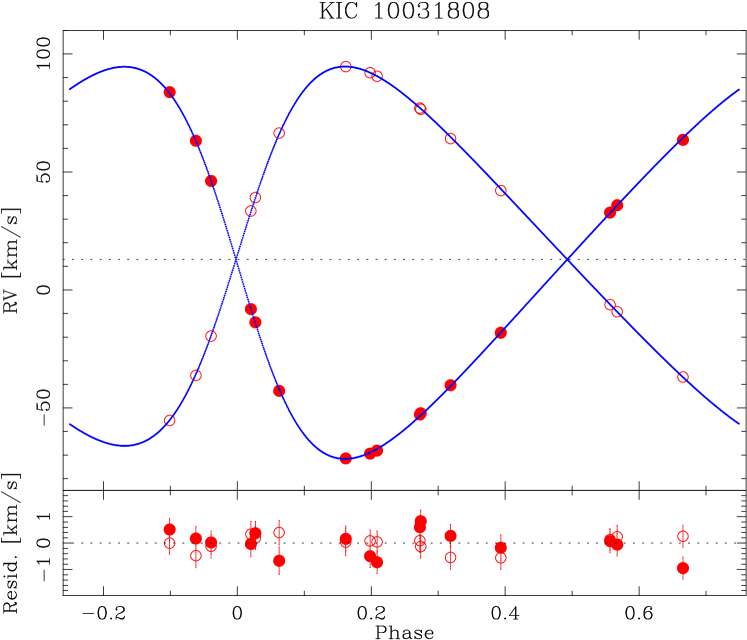
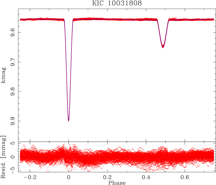
This is the only star in our sample that does not have the temperature given in the KEBC. We took 16 HIDES spectra of this system. Despite the two minima are separated in phase by nearly 0.5, a significant eccentricity was found in the LC modelling, that was nicely reproduced by the RVs. We had to fix when fitting each quarter light curve separately, but we perturbed it during the RS stage. We also found small non-zero values of the reflection coefficients: and .

Results of the modelling are presented in Figure 6, and parameter values can be found in Table 2. We found that the two stars are already evolved, currently at the end of the main sequence just before the transition to the giant branch. The more massive, larger component is cooler, and is the secondary in our nomenclature, because it is eclipsed during the shallower eclipse. We reached a very good precision in both masses (0.5-0.72 per cent) and radii (0.46-0.77 per cent), which makes our results useful for testing the evolutionary models of the final stages of the main sequence. Precision in masses is slightly affected by rotational broadening of the lines, but both components still seem to rotate slower than synchronously (from jktabsdim: and 18 km s-1 for the primary and secondary, respectively). Precision of radii (and other LC-based parameters) is also slightly hampered by additional photometric variability, although the of the light curve fit is relatively low.
We run a Lomb-Scargle periodogram on the LC residuals, and found numerous peaks at frequencies 2.5 d-1, with the highest one corresponding to the period of 2.363871 days. The corresponding variability amplitude is about 0.5 mmag (Fig. 7). We attribute it to pulsations rather than rotation, as a rotation with such period would translate into velocity of 55 or 65 km s-1, depending on the component. The lines we observe in the spectra are not broadened that much. This still could be explained by a spin-orbit misalignment, but the results from jktabsdim suggest alignment of orbital and rotational momenta after 50 Myr. Meanwhile, as mentioned before, the system appears to be much older (see also Sect. 5.2). The given period suggests a Doradus type of pulsations, and the lack of significant frequencies higher than 2.5 d-1 suggests no Scuti type variability. We did not perform a detailed frequency analysis for this system, as it is not the scope of this paper.
4.1.6 KIC 10191056 A
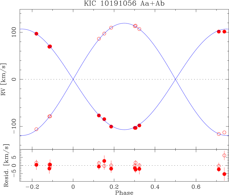
Another object in this study that was detected previously by the TrES survey. It is also one of the two with three sets of lines visible in the spectra. As in KIC 06525196, also in this case the third star is fainter than the two components of the eclipsing pair. It has been observed with HIDES eleven times. The spectral lines of the eclipsing binary are rotationally broadened, which is expected from tidally-locked components of a 2.42-day pair. This, and low of observations, hamper the precision of the RV-based parameters.
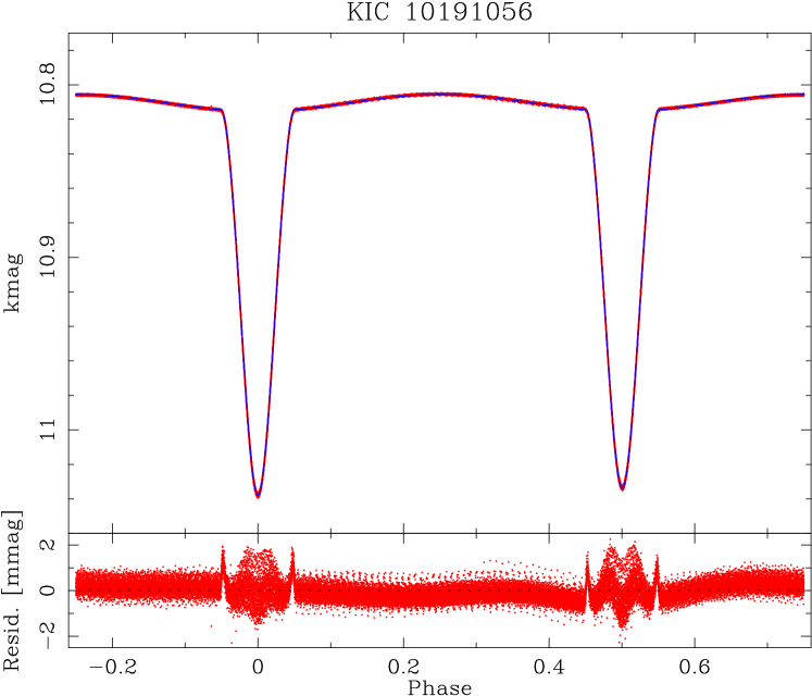
The Kepler light curve, on the other hand, is only weakly affected by variability of a kind other than eclipses and ellipsoidal variations, like spots or oscillations. Their amplitude is only about 1 mmag. It is in agreement with the fact that KIC 10191056 has the highest value of listed in the KEBC among our targets. The LC is more affected by some other systematic effects, like incorrect de-trending. For this reason we removed from the LC the data from quarters 14-17, and small pieces from quarters 2 and 10, still leaving almost 44000 data points from quarters 0 to 11 (there are no long-cadence data from quarters 12 and 13).
The careful analysis of the LC also revealed that the orbit is actually not circular. There is a small displacement of the secondary eclipse from the exact phase 0.5, by 18.7 min, or 0.00053 . The measurements of eclipse times, given separately for the primary and secondary by Gies et al. (2015), seem to confirm that by showing a gradual diverging, which suggests apsidal motion. The RV fit was therefore done with values of and fixed to those found in the LC fit. The ETVs of Gies et al. (2015) also show a small curvature (non-zero time derivative of the orbital period, ), which can be explained either by a presence of a third body, or a mass transfer. The latter seems unlikely, as the stars are far from filling their Roche lobes, and a clear detection of a third set of lines in the spectra supports the former scenario. The model presented in Figure 8, with parameters listed in Table 2, has been prepared under this assumption, i.e. the third light and linear variation of the systemic velocity have been accounted for. See Section 4.2.2 for the discussion of the motion of the companion.
We have reached a satisfactory precision of 2.0–2.5 per cent in masses, and a slightly better level of 1.3–1.7 per cent in radii, hampered mainly be the uncertainty in the third light. The uncertainty in mass already takes into account the error in the linear trend, which is discussed in Section 4.2.2.
4.1.7 KIC 10987439
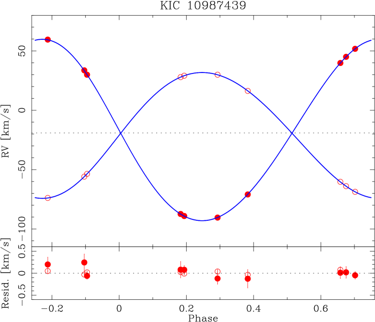
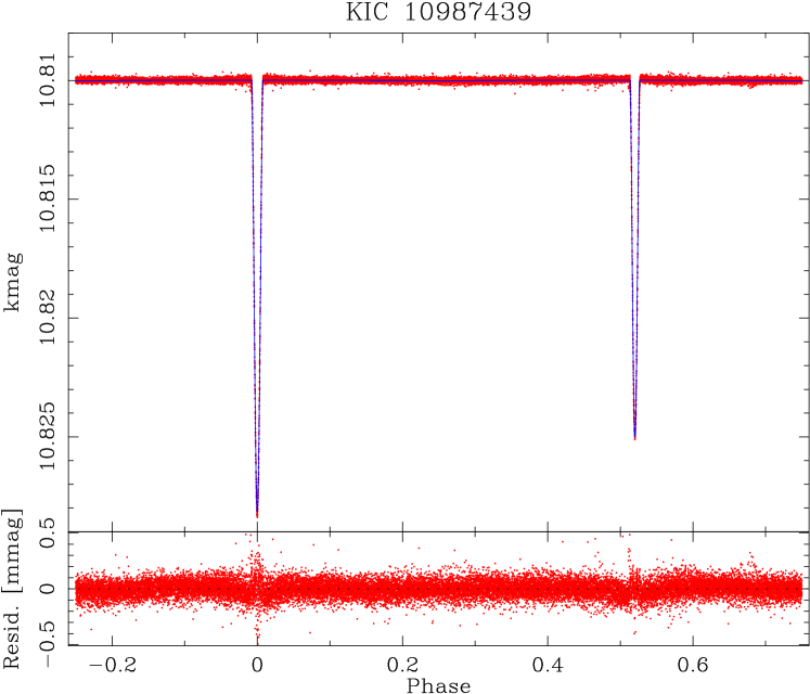
This system has the lowest amplitude of the out-of-eclipse variability in our sample, resulting in the smallest of the LC model 0.072 mmag ( ppm in flux). Also, the amount of photometric data is the lowest – only 25000 long-cadence measurements from quarters 1, 5, 9, 10, 13, 14, and 17, and no short-cadence data at all.
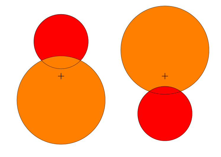
Despite similar depth of the eclipses, the pair turned out to be composed of quite different stars, and, to our initial surprise, it is the cooler, smaller, and less massive component that is eclipsed during the primary (deeper) minimum. This is because of a projection effect, caused by a small, but measurable eccentricity, and inclination relatively far from 90 degrees (see Fig. 10). The eclipses are shallow and only grazing, the primary one lasts about 20 per cent longer, and larger part of the stellar disk is obscured.
The spectroscopic data are also of a very good quality. The star has been observed ten times with HIDES. Narrow spectral lines made it possible to achieve the best RV precision in our sample for a single component, with the of 42 m s-1 for the component that contributes more to the system’s total flux (86.5 per cent), but is the secondary according to our convention. This is the level of RV precision we reached for RV standards (see Paper I). We also reach quite a good of 129 m s-1for our faint primary.
The light and RV curves are shown in Figure 9, and the system’s parameters can be found in Table 2. As in the case of KIC 10031808, we had to fit for reflection coefficients, and found them to be and for the primary and secondary, respectively. We reached a very good precision in masses: 0.33 per cent for both components, but a significantly worse in radii: 1.6–2.0 per cent. This seems surprising considering the excellent of the LC fit, but it may be understood when one takes the grazing eclipses into account. In such situations, there is not only a strong degeneration of the orbital inclination with the ratio of the radii , but also with their sum (). A small change in leads to a change in that is relatively large, in comparison to a situation when the eclipses are nearly central. Still, our results are good enough for meaningful tests of stellar evolution models.
There is also some leftover variability in the LC’s residuals. Larger scatter around the primary minimum suggests presence of small, migrating spots on the surface of the primary, whose spectral type is probably late G or early K. Due to the lack of short-cadence data, the spots can not be properly monitored, therefore we have removed about 20 most deviating data points from the minima, as they were causing the model to underestimate the eclipses’ depths, and hampering the results. Outside of the eclipses there is also a periodic modulation of an amplitude of 0.032 mmag present, and probably weak flares. The latter, if present, were however short-lasting, and, with the 30 min data cadence, covered by only 1-2 data points. The periodic modulation may be produced by spots, but with period of 1.624 days this would imply an asynchronous rotation with velocities of the order of 20 km s-1. We do not observe lines broadened that much – the stars rather seem to rotate synchronously. The planes of rotation may still be different than the orbital plane, but the orbit itself is nearly-circular, and, according to the theory of tidal interactions, the circularisation of the orbit occurs much later ( yr) than synchronisation of orbital and rotational periods, and spin-orbit alignment ( yr).
4.1.8 KIC 11922782
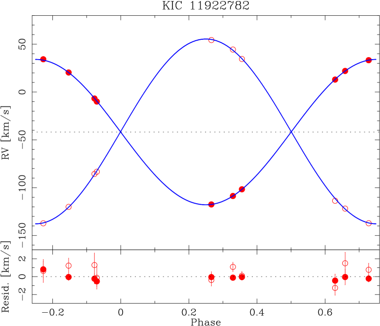

The last system in our sample, and the third common with Devor et al. (2008), was observed with HIDES ten times. The model we obtained for this pair is presented in Figure 11, with parameters listed in Table 2. We have reached a very good precision in masses (0.7-0.9 per cent), but significantly worse in radii (3.8-7.4), hampered mainly by spots evolving in time (note the large of the LC fit). This system also has one of the lowest mass ratios, and the highest contrast (in terms of luminosity ratio) between the components, which is reflected by very different -es in the RV fit, and contributed to large uncertainties of the LC-based parameters. The secondary is also the lowest-mass star we have analysed in this paper, (0.835 M⊙) and discrepancies between the observed and theoretically predicted radius are expected. The primary’s mass is very close to solar, but its radius is much larger, therefore we probably deal with an evolved version of our Sun. It is therefore an interesting system for further studies.
The light curve is strongly affected by rapidly evolving spots, located on both components, which can be deduced from variations in the depth of both minima. In order to confirm the chromospheric activity, we examined the Hα lines in our spectra, but found no obvious emission features, although the is not optimal, and the primary’s absorption line may be partially filled. As mentioned before, the Ca II H and K lines are not in the HIDES wavelength range.
4.2 Tertiary components
In this section we focus on the motion of the outer components of two triples: KIC 06525196 and 10191056. We follow the convention that the outer star is designated as the component B, and the inner eclipsing binary as A (= Aa+Ab).
4.2.1 The outer orbit of KIC 06525196
| This | Rappaport et al. | Borkovits et al. | |
|---|---|---|---|
| Parameter | work | (2013) | (2016) |
| (d) | 418.0(4) | 415.8(-) | 418.2(1) |
| (JD-2450000) | 6746.7(9) | 6805 | 6743(3) |
| (km s-1) | 11.67(12) | — | — |
| (km s-1) | 30.15(17) | — | — |
| 0.3872(45) | 0.61 | 0.41(6) | |
| 0.301(3) | 0.30 | 0.295(5) | |
| (∘) | 276(1) | 285 | 274(2) |
| (km s-1) | 4.58(4) | — | — |
| (M⊙) | 1.981(30) | 0.85 | — |
| (M⊙) | 0.767(14) | 0.59 | — |
| (AU) | 1.532(8) | — | — |
| (∘) | 84.7 | — | 80(-) |
| (M⊙) | 2.0063(67)a | — | 2.0(5) |
| (M⊙) | 0.777(12)b | — | 0.8(2) |
| (AU) | 1.539(10) | — | 1.55(13) |
| (km s-1) | 0.182 | — | — |
| (km s-1) | 0.096 | — | — |
a Directly from Table 2. b From and

This is a case of a triple-lined spectroscopic system, for which velocities of all stars were measured. The parameters of the outer orbit were previously estimated from ETVs (Rappaport et al., 2013; Borkovits et al., 2016), and the period is short enough to be covered with observations during only few semesters. We assumed that the outer orbit is Keplerian, as the distance to the third star B is much larger than the separation between Aa and Ab. In other words, we treated the outer A+B pair as a binary, but as the RVs of A we used the Aa+Ab systemic velocity measurements, calculated using the Equation 2. These measurements are also listed in Tab. 8.
The results are summarised in Table 4, and presented in Figure 12. As previously, uncertainties include systematics calculated with a bootstrap routine. Among other parameters, we show times of the pericentre passage , and the pericentre longitude given for the centre of mass of the inner binary. We also give the systemic velocity of the whole triple as . Because absolute mass of A is known (Tab. 2), we could calculate the inclination of the outer orbit, and found that the orientation is nearly edge-on, and is possible. There are however no signs of tertiary eclipses, nor eclipse depth variations, suggesting large mutual inclination . Such a scenario has been found by Rappaport et al. (2013), who give between 22.6 and 33.9∘, but other parameters show that their solution is only in a marginal agreement with ours. Moreover, their analysis of the LC led to very different values of the mass ratio of the inner binary, and third-light contribution: 0.71(1) and 0.024(1), respectively.
In much better agreement with ours are the parameters given by Borkovits et al. (2016). They, however, assume the mutual inclination to be zero, and argue that a small non-zero value () would produce significant eclipse depth variations, and that their solution rules out large values of . Table 4 shows a comparison of our results with those obtained by Rappaport et al. (2013) and Borkovits et al. (2016).
In the Paper I we have introduced a method to translate the observed ETVs to RVs of the centre of mass of the eclipsing binary. With the solution of the outer orbit known quite well, KIC 06525196 appears to be a good example to test this method of translation. We calculated our own ETVs, using the method described in the Section 3.3. We show them in Figure 13. They are consistent with those from Rappaport et al. (2013) and Borkovits et al. (2016) in terms of the orbital period (418 d) and total amplitude (250 s). However, by translating them directly to the RVs, we get a result that is not consistent with what we have measured (Fig. 12). The amplitude is larger (13 km s-1), and there seems to be a shift in phase.
It is because the ETVs in this system are caused by two effects – the ‘classical’ light time travel effect (LTTE, a.k.a. the Römer delay), and dynamical perturbations from the third body. Rappaport et al. (2013) clearly distinguish the contribution of those two effects, and in their Figure 2 one can see that their maxima are shifted in the orbital phase. They also give values of amplitudes of the two effects separately: 215 s for the LTTE, and 127 s for the dynamical (Borkovits et al. only give their ratio). Using the Equation 8 from Paper I, we can estimate the RV amplitude expected from the LTTE to be 11.76 km s-1, which is very close to what we have actually given in Table 4. The corresponding RV curve is also drawn in Fig. 12 as the black dashed line. It is similar to our solution, with the main discrepancy coming probably from a different period and moment of periastron passage. This case clearly shows that the RV motion of the centre of mass (variations of the systemic velocity of the inner binary) corresponds to the Römer delay only, and the direct translation of the ETVs to the RVs can only be done when the two effects are separated, or the dynamical one is negligible.
We can clearly see the advantage of direct RV measurements of three stars, as the results obtained in this study are much more precise (1.5 per cent in ) than from eclipse timing variations. However, the analysis of ETVs gives a slightly different set of orbital parameters, and takes into account more effects. Both approaches are therefore complementary, and together allow for a complete description of the system’s dynamics and orbital architecture. With all masses directly and precisely measured, KIC 06525196 is a unique system, important to study formation and dynamical evolution of multiples.
4.2.2 The tertiary of KIC 10191056
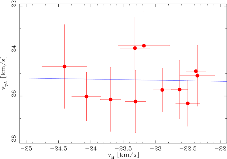
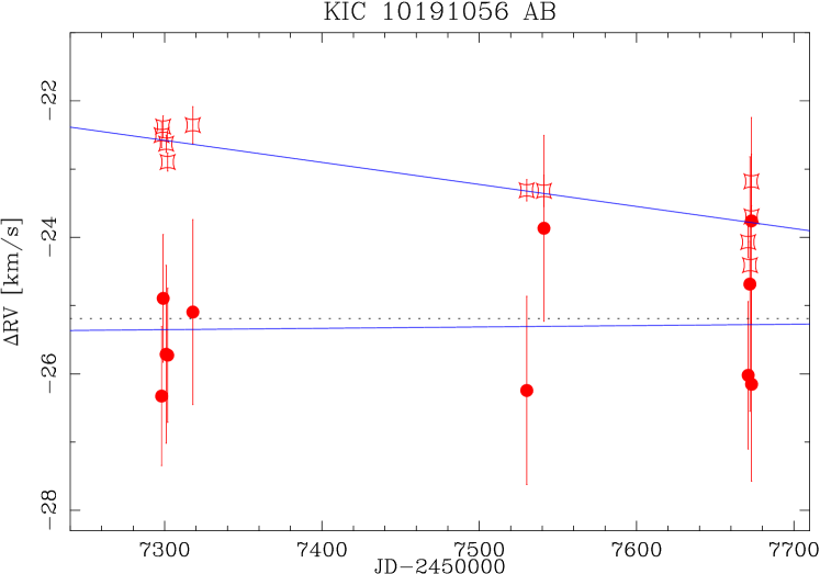
For the analysis of the inner eclipsing pair in this triple-lined system we assumed that the two components resolved in high-angular-resolution imaging are gravitationally bound and that the fainter star B is the source of the narrow spectral lines. We also assumed that the change of its velocity () is linear, as is the change of the systemic velocity of the inner pair A (). This is supported by the fact, that in 33 years the position of B relatively to A has not changed much, and the RVs of the tertiary are close to the systemic velocity of A.
We first calculated for each observation, using the Equation 2. Then we fitted a linear trend our measurements of , obtaining km s-1 d-1 ( km s-1). We have then estimated the mass ratio , and the systemic velocity of the whole system , by using a modified Equation 2:
| (3) |
in which we substituted and with and , respectively. The linear regression to this equation is shown in Figure 14. We found km s-1, and ( km s-1), the mass of the tertiary is therefore M⊙. This value is in general agreement with the fact that the tertiary is fainter than each of the eclipsing components, however seems to be too low for the observed magnitude differences, and the formal uncertainty is very large due to the errors of individual measurements, coming from individual errors of and . It is thus formally possible, that the tertiary is more massive, but other observational facts do not support this. We have, however, decided to keep this conservative uncertainty in further analysis. Finally, we have estimated the scale of the linear trend km s-1 d-1. The trend is, therefore, undistinguishable from zero. This is the value we used for the orbital fit described previously, and its uncertainty has been properly taken into account. Our measurements of and , and both linear trends are shown in Fig. 15. However, because is indistinguishable from zero, its confirmation requires further observations in the future.
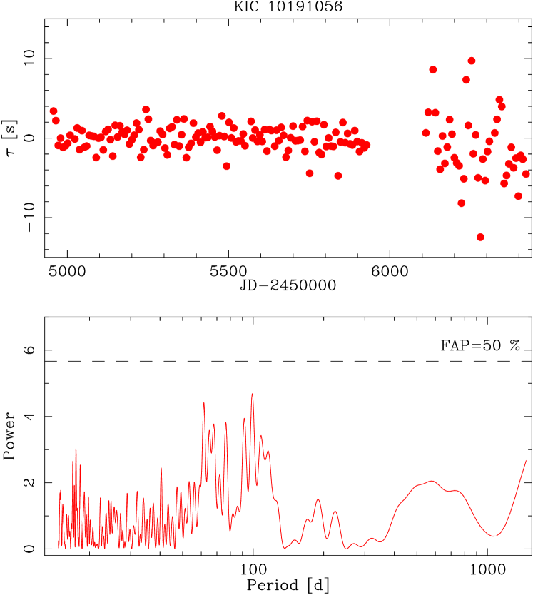
Having means that the tertiary is in fact not gravitationally bound (a blend), or the period of the AB orbit is too long to see the motion in the RVs. We mentioned before that the ETVs reported by Gies et al. (2015) show a small curvature, as well as a gradual diverging. We have calculated our own ETVs, which we present in Figure 16. Please note that the corresponding periodogram shows no statistically significant peaks, meaning no short-period variations in KIC 10191056. We also do not see any curvature, down to the level of 2.5 s ( of our measurements) over the whole course of Kepler observations, and even 1.4 s for data taken before JD=2456000. The ETVs from Gies et al. (2015) vary by about 8 seconds, so we should be able to see the change. The reason why our results differ from those of Gies et al. (2015) remains unclear to us.
Please also note that the measured visual separation between A and B has changed only by 0.16 arcsec in 33 years, but it can be explained by the absolute proper motion of the system, which is mas/yr (Gaia Collaboration, 2016). If A and B are not gravitationally bound, or the period of their common orbit is too long for a detection of any motion in RVs or ETVs, there might be another body causing the variation in the tertiary’s velocity. It might produce a linear trend, but there is also a possibility that the variation is short-period, and we have also investigated this scenario.
| Parameter | Sol. 1 | Sol. 2 | Sol. 3 | Sol. 4 |
|---|---|---|---|---|
| (d) | 9.892(25) | 10.220(17) | 17.887(37) | 18.92(10) |
| (JD-2457200) | 97.1(1.2) | 83.0(1.0) | 97.66(44) | 98.4(7.1) |
| (km s-1) | 1.05(20) | 1.09(21) | 0.95(22) | 1.01(25) |
| (km s-1) | -23.21(8) | -23.08(7) | -23.28(9) | -23.50(17) |
| 0.39(26) | 0.41(14) | 0.65(21) | 0.11(24) | |
| (∘) | 247(22) | 161(24) | 272(17) | 341(164) |
| (m s-1) | 199 | 189 | 217 | 215 |
| (M | 10.2(2.3) | 10.6(2.3) | 9.3(2.8) | 13.2(3.4) |
a Assuming mass of the host star =1 M⊙.

The two points with the highest values, and the ‘curvatures’ seen in the first and last four measurements, limit the possible periods to the range of 7–23 days. We have explored this range of periods and found several values, that give satisfactory orbital fits. They are listed in Table 5, together with other (putative) orbital parameters, and also plotted on Figure 17. Please note that, except the last one, all solutions predict significant eccentricity. Assuming mass of the central star to be 1 M⊙, all solutions lead to the lower mass limit of the companion in the planetary regime. Such a planet would be the first one found around a blend with (or a very wide companion to) an eclipsing binary. For the record, under the assumption of no linear trend, the systemic velocity of the eclipsing pair is km s-1, and the two velocity amplitudes are exactly the same as in Table 2.
We would like to stress that these ‘planetary’ solutions are highly uncertain due to small number of measurements. We also find the scenario with a linear trend in more probable, however our current data do not allow to confirm it securely.
5 Discussion
5.1 Comparison with the TrES results
| KIC | 08552540 | 10191056 | 11922782 |
|---|---|---|---|
| T- | Lyr1-00359 | Lyr1-00687 | Cyg1-00246 |
| (d) | 1.061932(9) | 2.427610(34) | 3.512815(70) |
| (JD-2454900) | 54.102(12) | 55.0970(23) | 56.188(35) |
| 0.0(fix) | 0.003(fix) | 0.0(fix) | |
| (∘) | — | 278(7) | — |
| 0.2426(42) | 0.175(13) | 0.127(21) | |
| 0.1841(54) | 0.154(15) | 0.084(22) | |
| (∘) | 85.65(98) | 82.24(37) | 83.9(1.2) |
| 0.91(11) | 0.968(28) | 0.401(25) | |
| 0.305(13) | 0.77(30) | 0.19 | |
| 0.0(fix) | 0.0(fix) | 0.16 | |
| (mmag) | 18.0 | 6.6 | 7.9 |
| Parameter | This work | Devor et al. (2008) |
|---|---|---|
| T-Lyr1-00359 = KIC 08552540 | ||
| (d) | 1.06193441(4) | 1.061922(15) |
| (M⊙) | 1.153(36) | 1.655(15) |
| (M⊙) | 0.956(28) | 1.296(12) |
| T-Lyr1-00687 = KIC 10191056 | ||
| (d) | 2.427494881(19) | 2.427512(79) |
| (M⊙) | 1.575(30) | 1.209(13) |
| (M⊙) | 1.420(36) | 1.208(13) |
| T-Cyg1-00246 = KIC 11922782 | ||
| (d) | 3.5129340(4) | 3.51306(16) |
| (M⊙) | 1.065(10) | 1.498(26) |
| (M⊙) | 0.835(6) | 0.970(32) |
Three of our systems have additional photometric data available from the TrES survey, and the catalogue of eclipsing binaries prepared by Devor et al. (2008). We have fitted model LCs to these data, using the jktebop code in almost the same way as for the Kepler photometry (the differences were that the TrES LCs were not divided into smaller subsets for the RS stage, the small eccentricity of KIC 10191056 was held fixed, and third light of KIC 11922782 was fitted for, due to much shallower eclipses in the TrES curve). The results are listed in Table 6. For most of the parameters independent from the bandpass (i.e. ) the agreement is well within the given 1 uncertainties. The results from Kepler photometry are also significantly more precise, with the exception of KIC 08552540, which is the system with the largest spot-originated brightness variations in the sample, and for which the Kepler -based results are only slightly better. This case shows that even with such an exquisite instrumental precision, the resulting parameters may still not be derived as well as expected, unless the additional variability is removed carefully and correctly.
Notably, in case of KIC 11922782 the is essentially the same for TrES and Kepler LCs, but the TrES results were hampered by the third light, and the fact that over the course of the observations the spot-originated modulation did not change much, while it did in Kepler observations, and therefore could be averaged over the orbital phase. The TrES LC clearly shows systematic residuals (Fig. 18, bottom). An alternative explanation for shallower TrES eclipses may be a change in orbital inclination. We, however, find it unlikely, despite such cases being observed by Kepler (Slawson et al., 2011; Rappaport et al., 2013). The TrES measurements were done with a relatively large 30”30” photometric aperture, and a different, i.e. smaller inclination would produce eclipses that last shorter, but we don’t see such effect. The best fit was found for third light contribution of over 15 per cent, although with a very large uncertainty.
In their work Devor et al. (2008) also used their LCs to derive stellar masses. They used the meci code (Devor & Charbonneau, 2006), which looks for the most probable combination of two masses and age of the system, by comparing global photometric properties (brightness and colours) with a set of isochrones. Having our HIDES spectroscopy and RVs, we can compare our direct determinations of masses with their indirect results. Such comparison is shown in Table 7. One can quickly note that the masses found indirectly are in a strong disagreement with our findings. This is, however, not the first example of such a discrepancy that can be found in literature. The same meci method (with small modifications) was used later for example by Hełminiak et al. (2013) on a sample of DEBs from the Galactic bulge, or by Lee (2015) on ASAS, NSVS, and LINEAR systems. While the Galactic bulge systems do not have their spectroscopy done so far, many of the ASAS ones from Lee (2015) have their parameters published (e.g. Dimitrov et al., 2014; Djurašević et al., 2011; Hełminiak et al., 2009, 2015a; Ratajczak et al., 2013, 2016; Różyczka et al., 2013).
There are also many systems whose light curves alone were analysed with other codes, like phoebe (Prša & Zwitter, 2005). This code works on Kopal modified potentials, which are dependent on the mass ratio, and determine the shape of the out-of-eclipse ellipsoidal variations. It is therefore theoretically possible to estimate for systems showing this phenomenon. In few cases, a complete LC+RV analysis have also been performed, and masses and/or their ratios found both ways can also be compared, like KIC 06525196 in this work vs. Rappaport et al. (2013).
Such a comparison between the direct and indirect measurements is not the main scope of this paper. Here we only conclude, that there is very little agreement between direct and indirect mass and mass ratio determinations, and if there is, it is either accidental, or due to very large uncertainties of the indirect one. This means that the LC-only results are very insecure and should be treated with a lot of caution.
5.2 Age, evolutionary status, , and distance

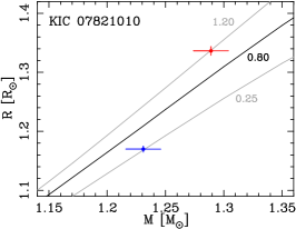
In this Section we asses the age and evolutionary status of each system by comparing our results, namely masses and radii, with the theoretical PARSEC isochrones (Bressan et al., 2012), that include calculation of absolute magnitudes in the Kepler photometric band. From the best-matching isochrone we estimate the effective temperatures, and use them to infer distances with jktabsdim. We compare these distances with the recently published Gaia Data Release 1 (GDR1; Gaia Collaboration, 2016), which gives results of the Tycho-Gaia Astrometric Solution (Michalik et al., 2015).
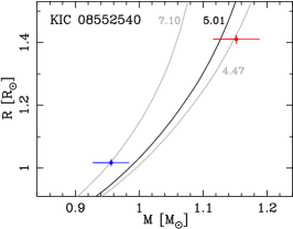
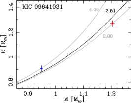
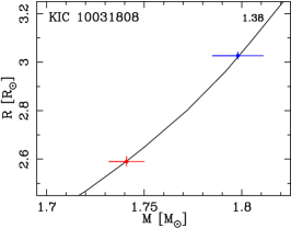
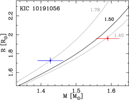
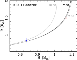
In Figure 19 we present our results of isochrone fitting on mass-radius planes. We’d like to remind that these result assume solar metallicity, therefore the ages should be treated with some caution, because of the age-metallicity degeneration. These results could be corrected if precise multi-band light curves were obtained, and system’s metallicity and temperatures of both components independently estimated.
5.2.1 KIC 06525196
It is a problematic system for two reasons. First, it is a triple and we only have information of fractional fluxes in the Kepler band, not in (no multi-band photometry). Therefore we could not calculate the distance with the jktabsdim code. Fortunately, we know the mass of the third star precisely, (with 1.5 per cent relative precision, see Tab. 4) which helped to put some additional constraints. Second, the relatively large uncertainties of radii, and the fact that in our solution the less massive secondary turned out to be formally larger, caused that two scenarios were possible for this system: ‘young’ with the age of 20 Myr () indicating the pre-main-sequence stage, and ‘old’ with the age of 5.25 Gyr (). Comparison of predicted flux ratios for all three stars (from absolute magnitude differences) favoured the ‘old’ one, however the agreement was only marginal. In this scenario, the primary and secondary lay on isochrones of 4.0 Gyr () and 7.1 Gyr (), respectively.
The predicted temperatures are , , and K for the primary, secondary, and tertiary, respectively. The respective absolute magnitudes in the Kepler filter () are: 4.30, 4.75, and 6.23 mag, with 0.20 mag uncertainty for all components. Large errors in radii lead to large uncertainties in absolute magnitudes. Also the error of from our jktebop solution is significant. We suspect that its value, as well as the value of , might be overestimated. The predicted total is mag. By comparing it with the observed , we obtain the distance pc, assuming no extinction. Taking this value, and the physical size of the major semi-axis AU, we can calculate its angular size: mas. The resulting distance is in a very good agreement with the GDR1 value of pc, which confirms the correctness of our solution and usage of the solar-metallicity isochrone. Notably, with its physical parameters, and probable metallicity and age, the primary can be considered a solar analogue.
5.2.2 KIC 07821010
Comparison of our results with solar metallicity PARSEC isochrones on the plane shows that both components are on the main sequence. The isochrone that fits best to the whole system is found for the age of 800 Myr (). The primary and secondary components lay on isochrones of 1.20 Gyr () and 250 Myr (), respectively. The predicted effective temperatures are and K. We use them and the available photometry as the input for jktabsdim to estimate the and distance. We found that the best consistency between various bands is found for , and the resulting distance is pc. The GDR1 distance – pc – is in a formal agreement, however significantly less precise.
5.2.3 KIC 08552540 (V2277 Cyg)
This system turns out to be relatively old, and is a good example of how fast rotation (due to tidal locking) can help sustain a high level of activity in mature, solar-like stars. The comparison with isochrones suggests the age of 5.01 Gyr (). The primary and secondary lay on isochrones of 4.47 Gyr () and 7.1 Gyr (), respectively. Their predicted temperatures are and K. The distance, as calculated by the jktabsdim code, is pc, with no extinction. The small error comes from the very consistent values individually calculated for each band.
The jktebop analysis of and -band curves from ASAS-K, gives respective observed magnitudes of and mag for the primary, and and mag for the secondary. This leads to the colours of and mag for the primary and secondary, respectively. The second value has its uncertainty too large to be useful to constrain the temperature. The first one alone may be used to assess the interstellar reddening. The 7.1 Gyr PARSEC isochrone gives mag for the primary’s mass, which is close to, but not exactly the value we got from the ASAS-K data. The is therefore 0.031 mag, which translates into mag. By putting this value in jktabsdim we obtain the distance of pc, which is in a very good agreement with our previous value, but has larger uncertainty.
However, the GDR1 distance is pc, so the agreement is only in a 2 level. If a different metallicity isochrone was used, the predicted temperatures could have been lower, resulting in a smaller jktabsdim distance.
5.2.4 KIC 09641031 (FL Lyr)
Our mass and radius measurements are best reproduced by a 2.51 Gyr () isochrone. The agreement is at a 1 level, and is better than if the original results of Popper et al. (1986) were compared with the PARSEC set. Individually, the components lay on isochrones of 2.00 (, primary) and 4.00 Gyr (, secondary).
This is a special case in our sample, as it is the only system with independent estimates of the effective temperatures: and K for the primary and secondary, respectively (Popper et al., 1986). We used them together with total system’s brightness in as an input in jktabsdim, and calculated the distance. We obtained the weighted average value of pc (no extinction), which is in excellent agreement with the Hipparcos value of pc (van Leeuwen, 2007), and only marginal with the GDR1 value of pc. Parameters from the original solution of Popper et al. (1986) give a slightly higher value of pc. This may be an indication that our solution is less accurate.
For the record, the temperatures predicted by the best-fitting isochrone are and K for the primary and secondary, respectively. A good consistency in distance calculation is reached for , which results in pc – closer to the GDR1 value than for the Popper’s temperatures. In any case, despite a significantly different temperature scale, all the results are still in agreement with the ones given above. The consistency between distances calculated for different passbands is also very high. To confirm which distance is the correct one, the Gaia satellite will have to provide its determination at the level of 1 pc, or mas in parallax, which can be expected from the future data releases.
5.2.5 KIC 10031808
Comparison of our results with the solar metallicity PARSEC isochrone on the plane shows a very good agreement for an age of 1.38 Gyr () – both components are located on this line. Both are already somewhat evolved and are about to leave the main sequence, which makes this system important for studying late phases of main sequence evolution. In this stage the age-metallicity degeneracy is weaker than for earlier ages, as the slope of the isochrone on the plane changes with the metal content. With masses and radii precise enough, one could constrain [] quite securely. In this case, however, the agreement is already excellent, meaning that the system’s true metallicity is close to solar. The model predicts temperatures of and K for the primary and secondary, respectively. When incorporated into jktabsdim, they result in pc for mag. The GDR1 value of pc agrees quite well, however mainly because of the large uncertainty.
One should note that the temperatures, and values of (Tab. 2) place both components in Scuti and/or Doradus instability strips (Kahraman Aliçavuş et al., 2016). As shown in Section 4.1.5, we identified many modes of Dor type pulsations in the residuals of the LC fit, while Scuti are not seen. We can therefore conclude that at least one component is a Dor variable. This makes KIC 10031808 even more interesting, as examples of such stars in eclipsing systems, especially with well measured parameters, are very rare (e.g. Debosscher et al., 2013; Guo et al., 2016).
5.2.6 KIC 10191056
The two eclipsing components of this triple seem to be coming to an end of their main sequence evolution. The system’s parameters are consistent with a 1.50 Gyr () isochrone, while the the primary and secondary are better individually represented by 1.40 Gyr () and 1.78 Gyr () lines, respectively.
The predicted temperatures are K, and K. We can use them in jktabsdim to estimate the distance to the system, but only with magnitudes in and , as the ASAS-K data allow us to estimate the tertiary’s contribution only in those bands. We found that the and observed magnitudes of the three components are: and mag for the primary, and mag for the secondary, and and mag for the third star. Unfortunately, the resulting colours – , , and mag for the primary, secondary and tertiary, respectively – are not precise enough to put any constraints on the effective temperatures.
After correcting for the third light, and assuming no interstellar extinction, we obtain the distance of pc, which is the largest one in our sample. When the distance is estimated from the observed contributions to the flux in the Kepler band, and compared with absolute values from the isochrone, we obtain a similar value of pc. If we want to force the distances calculated in jktabsdim for and -band individually to be equal, we must assume mag. In such case, we obtain pc. Comparison with the GDR1, which gives pc, suggests that this is a better approach, but the large uncertainty makes it not completely conclusive. However, no interstellar extinction at such a distance seems unlikely.
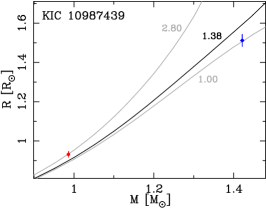
5.2.7 KIC 10987439
This system is interesting as it has the smallest mass ratio (when defined as the smaller mass over the larger) in our sample. In principle it is more difficult to fit a single isochrone to two points laying far from each other on the – or Hertzsprung-Russell (H-R) diagram. In this case there is no solar-metallicity isochrone that matches both components at a 1 level.
These stars seem to reside on the main sequence. The best match to both of them simultaneously was found for the age of 1.38 Gyr (). The primary and secondary separately are best reproduced by the ages of 2.8 Gyr () and 1.0 Gyr (), respectively. The system is not active, therefore this large discrepancy (note small mass and radius errors) can not be attributed to spots. We presume that the two components have different values of the mixing length parameter . Such a solution has been proposed to explain the observed properties of several F,G,K-type stars in eclipsing binaries (e.g. Clausen et al., 2009; Vos et al., 2012).
The best-fitting isochrone predicts effective temperatures of and K. This results in the jktabsdim distance of pc, at mag. In this case the agreement with GDR1, which gives pc, is also very good.
5.2.8 KIC 11922782
The last system in our sample is also the oldest one. The observed masses and radii are very well reproduced by a 7.50 Gyr isochrone (), while primary and secondary formally lay on isochrones of 7.35 Gyr () and 10.0 Gyr (), respectively. The former has already evolved out of the main sequence, and constrains the age much stronger than the secondary. With the mass very close to 1 M⊙, but a significantly larger radius, it can serve as an insight into the state of our Sun in few billion years. Despite relatively large uncertainty in radius, the secondary seems to follow the trend observed in many low-mass, active components of short-period eclipsing binaries, that the observed radius is larger than expected from isochrones.
The predicted temperatures are and K for the primary and secondary, respectively. The distance is therefore pc, at mag. There is no solution for this system in the GDR1.
6 Summary
We have studied six double- and two triple-lined detached eclipsing binaries from the KEBC database, for which we obtained absolute values of masses and radii, and estimated other parameters from the comparison with theoretical isochrones. We also conclude that stellar masses determined indirectly (without RVs), with the exception of asteroseismology, are not reliable. Eclipse timing variation analysis of selected targets was also performed.
In some cases we have managed to reach precision good enough to test the models. The PARSEC models managed to reproduce our results quite well. Each best-fitting isochrone agreed with our masses and radii within 3. The differences can be attributed to the true metallicities being different from solar, and/or to different mixing length parameters for each component of a given pair. Also the estimated distances were in good agreement with those from GDR1, which for the largest distances turned out to be much less precise than our results.
In this work we managed to identify interesting targets, worth further studies. In our sample we see various classes of objects, like low-mass stars (e.g. KIC 11922782), a Dor pulsator (KIC 10031808), or a hierarchical triple with nearly complete dynamical description (KIC 0652196 AB). Further work on these objects should focus on spectroscopic analysis, in order to independently determine temperatures and metallicities, multi-colour photometry, and precise correction of brightness variations (spots, pulsations) in order to improve the precision in radii. Also, a long-term spectroscopic monitoring of the unsolved case of KIC 10191056 B, and a detailed frequency analysis of KIC 10031808 are encouraged.
Acknowledgments
We would like to thank the anonymous Referee and Prof. Andrzej Pigulski from the Astronomical Institute of the Wrocław University, for fruitful discussions and valuable suggestions.
This research has made use of the SIMBAD database, operated at CDS, Strasbourg, France. This work has made use of data from the European Space Agency (ESA) mission Gaia (http://www.cosmos.esa.int/gaia), processed by the Gaia Data Processing and Analysis Consortium (DPAC, http://www.cosmos.esa.int/web/gaia/dpac/consortium). Funding for the DPAC has been provided by national institutions, in particular the institutions participating in the Gaia Multilateral Agreement.
KGH acknowledges support provided by the National Astronomical Observatory of Japan as Subaru Astronomical Research Fellow. This work is supported by the Polish National Science Center grants 2011/03/N/ST9/03192 and 2015/16/S/ST9/00461, by the European Research Council through a Starting Grant, by the Foundation for Polish Science through ‘Idee dla Polski’ funding scheme, and by the Polish Ministry of Science and Higher Education through grant W103/ERC/2011.
References
- Akerlof et al. (2000) Akerlof C., et al. 2000, AJ, 119, 1901
- Alonso et al. (2004) Alonso R., et al., 2004, ApJ, 613, L153
- Armstrong et al. (2014) Armstrong D. J., Gomez Maqueo Chew Y., Faedi F., Polacco D., 2014, MNRAS, 437, 3473
- Beck et al. (2014) Beck P. G., et al., 2014, A&A, 564, A36
- Borkovits et al. (2015) Borkovits T., Rappaport S., Hajdu T., Sztakovics J., 2015, MNRAS, 448, 946
- Borkovits et al. (2016) Borkovits T., Hajdu T., Sztakovics J., Rappaport S., Levine A., Bíro I. B., 2016, MNRAS, 455, 4136
- Bradley et al. (2015) Bradley P. A., Guzik J. A., Miles L. F., Uytterhoeven K., Jackiewicz J., Kinemuchi K., 2015, AJ, 149, 68
- Bressan et al. (2012) Bressan A., Marigo P., Girardi L., Salasnich B., Dal Cero C., Rubele S., Nanni A., 2012, MNRAS, 427, 127
- Clausen et al. (2009) Clausen J. V., Bruntt H., Claret A., Larsen A., ANdersen J., Nordström B., Gimenéz A, 2009, A&A, 502, 253
- Coelho et al. (2005) Coelho P., et al., 2005, A&A, 443, 735
- Conroy et al. (2014) Conroy K. E., Prša A., Stassun K. G., Orosz J. A. Fabrycky D. C., Welsh W. F., 2014, AJ, 147, 45
- Coughlin et al. (2011) Coughlin J. L., Lopez-Morales M., Harrison T. E., Ule N., Hoffman D. I., 2011, AJ, 141, 78
- Couteau (1983) Couteau P., 1938, A&AS, 53, 441
- Debosscher et al. (2013) Debosscher J., et al., 2013, A&A, 556, A56
- Devor & Charbonneau (2006) Devor J., Charbonneau D., 2006, ApJ, 653, 648
- Devor et al. (2008) Devor J., Charbonneau D., O’Donovan F. T., Mandushev G., Torres G., 2008, AJ, 135, 850
- Diethel (2001) Diethelm R. 2001, IBVS, 5060, 1
- Dimitrov et al. (2014) Dimitrov W., et al., 2014, A&A, 564, A26
- Djurašević et al. (2011) Djurašević G., Yılmaz M., Baştürk Ö., Kılıçoǧlu T., Latković O., Çalışkan Ş., 2011, A&A, 525, A66
- Gaia Collaboration (2016) Gaia Collaboration 2016, A&A, 595, A2
- Gies et al. (2015) Gies D. R., Matson R. A., Guo Z., Lester K. V., Orosz J. A., Peters G. J., 2015, AJ, 150, 178
- Gies et al. (2012) Gies D. R., Williams S. J., Matson R. A., Guo Z., Thomas S. M., Orosz J. A., Peters G. J., 2012, AJ, 143, 137
- Guo et al. (2016) Guo Z., Gies, D. R., Matson R. A., García Hernández, A., 2016, ApJ, 826, 69
- Hełminiak et al. (2009) Hełminiak K. G., Konacki M., Ratajczak M., Muterspaugh M. W., 2009, MNRAS, 400, 969
- Hełminiak et al. (2012) Hełminiak K. G. et al., 2012, MNRAS, 425, 1245
- Hełminiak et al. (2013) Hełminiak K. G., Devor J., Minniti D., Sybilski P. 2013, MNRAS, 431, 2024
- Hełminiak et al. (2015a) Hełminiak K. G. et al., 2015, MNRAS, 448, 1945
- Hełminiak et al. (2015b) Hełminiak K. G., Ukita N., Kambe E., Konacki M., 2015b, ApJL, 813, 25
- Hełminiak et al. (2016) Hełminiak K. G., Ukita N., Kambe E., Kozłowski S., Sybilski P., Ratajczak M., Maehara H., Konacki M., 2016, MNRAS, 461, 2896
- Izumiura (1999) Izumiura H., 1999, in: Proc. 4th East Asian Meeting on Astronomy, ed. P. S. Chen, Kunming, Yunnan Observatory, p. 77
- Kambe et al. (2013) Kambe E., et al., 2013, PASJ, 65, 15
- Kahraman Aliçavuş et al. (2016) Kahraman Aliçavuş F., et al., 2016, MNRAS, 458, 2307
- Kepler Mission Team (2009) Kepler Mission Team, 2009, VizieR Online Data Catalog, 5133, 0
- Kervella et al. (2004) Kervella P., Thévenin F., Di Folco E., Ségransan D., 2004, A&A, 426, 297
- Kirk et al. (2016) Kirk B. et al., 2016, AJ, 151, 68
- Klinglesmith & Sobieski (1970) Klinglesmith D. A., Sobieski S., 1970, AJ, 75, 175
- Konacki et al. (2010) Konacki M., Muterspaugh M. W., Kulkarni S. R., Hełminiak, K. G., 2010, ApJ, 719, 1293
- Kozłowski et al. (2011) Kozłowski S. K., Konacki M., Sybilski P., 2011, MNRAS, 416, 2020
- Kozyreva et al. (2015) Kozyreva V. S., Bogomazov A. I., Demkov B. P., Zotov L. V., Tutukov A. V., 2015, ARep, 59, 1036
- Kurucz (1992) Kurucz R. L., 1992, in Barbury B., Renzini A., eds, Proc. IAU Symp. 149, The Stellar Population of Galaxies, Kluwer Academic Publishers, Dordrecht, p. 225
- Lastennet & Valls Gabaud (2002) Lastennet E., Valls-Gabaud D., 2002, A&A, 396, 551
- Lee (2015) Lee C.-S. 2015, MNRAS, 453, 3474
- Mason et al. (2001) Mason B. D., Wycoff G. L., Hartkopf W. I., Douglass G. G., Worley, C. E., 2001, AJ, 122, 3466
- Matijevič et al. (2012) Matijevič G., Prša A., Orosz J. A., Welsh W. F., Bloemen S., Barclay T., 2012, AJ, 143, 123
- Morgenroth (1935) Morgenroth O., 1935, Astr. Nachr., 255, 425
- Michalik et al. (2015) Michalik D., Lindegren L., Hobbs D., 2015, A&A, 574, A115
- Orosz (2015) Orosz J. A., 2015, ASPC, 496, 55
- Pigulski et al. (2009) Pigulski A., Pojmański G., Pilecki B., Szczygieł D. M., 2009, AcA, 59, 33
- Popper & Etzel (1981) Popper D. M., Etzel P. B., 1981, AJ, 86, 102
- Popper et al. (1986) Popper D. M., Lacy C. H. S., Frueh M. L., Turner A. E., 1986, AJ, 91, 383
- Prša & Zwitter (2005) Prša A., Zwitter T., 2005, ApJ, 628, 426
- Prša et al. (2011) Prša A. et al., 2011, AJ, 141, 83
- Rappaport et al. (2013) Rappaport S., Deck K., Levine A., Borkovits T., Carter J., El Mellach I., Sanchis-Ojeda R., Kalomeni B., 2014, ApJ, 768, 33
- Ratajczak et al. (2013) Ratajczak M., Hełminiak K. G., Konacki M., Jordán A., 2013, MNRAS, 433, 2357
- Ratajczak et al. (2016) Ratajczak M. et al., 2016, MNRAS, 461, 2234
- Różyczka et al. (2013) Różyczka M., Pietrukowicz P, Kałużny J., Pych W., Angeloni R., Dékány I., 2013, MNRAS, 429, 1840
- Sharp et al. (2014) Sharp H. et al., 2014, AAS, 223, 155.23
- Slawson et al. (2011) Slawson R. W. et al., 2011, AJ, 142, 160
- Southworth (2015) Southworth J., 2015, ASPC, 496, 164
- Southworth et al. (2004a) Southworth J., Maxted P. F. L., Smalley B., 2004a, MNRAS, 351, 1277
- Southworth et al. (2004b) Southworth J., Zucker S., Maxted P. F. L., Smalley B., 2004b, MNRAS, 355, 986
- Southworth et al. (2011) Southworth J., Pavlovski K., Tamajo E., Smalley B., West R. G., Anderson D. R., 2011, MNRAS, 414, 3740
- Struve et al. (1950) Struve O., Horak H. G., Canavaggia R., Kourganoff V., Colacevich A., 1950, ApJ, 111, 658
- Tenenbaum et al. (2012) Tenenbaum P. et al., 2012, ApJS, 199, 24
- Torres et al. (2008) Torres G., Vaz L. P. R., Sandberg Lacy C. H., 2008, AJ, 136, 2158
- Torres et al. (2010) Torres G., Andersen J., Gimenez A., 2010, A&ARv, 18, 67
- van Leeuwen (2007) van Leeuwen F., 2007, A&A, 474, 653
- Vos et al. (2012) Vos J., Clausen J. V., Jørgensen U. G., Østensen R. H., Claret A., Hillen M., Exter K., 2012, A&A, 540, A64
- Wenger et al. (2000) Wenger M. et al., 2000, A&A, 143, 9
- Wilson (1941) Wilson O. C., 1941, ApJ, 93, 29
- Ziegler et al. (2017) Ziegler C. et al., 2017, AJ, 153, 66
- Zucker & Mazeh (1994) Zucker S., Mazeh T., 1994, ApJ, 420, 806
Appendix A RV measurements
In Table 8 we present individual RV measurements used in this work. Both KIC 06525196 and 10191056 have been treated as two SB2s, and the systemic velocities of their inner pairs are given in Tab. 8 as . Time stamp is BJD-2450000. Exposure times and around Å are also given.
| BJD | KIC | ||||||
|---|---|---|---|---|---|---|---|
| -2450000 | (km s-1) | (km s-1) | (km s-1) | (km s-1) | (s) | ||
| 6865.062301 | 58.509 | 0.232 | -35.422 | 0.312 | 6525196 A | 900 | 54 |
| 6865.220925 | 77.453 | 0.347 | -56.066 | 0.399 | 6525196 A | 1200 | 66 |
| 6866.000781 | 77.885 | 0.362 | -56.706 | 0.436 | 6525196 A | 1200 | 43 |
| … | |||||||
| 6865.062301 | 13.018 | 0.218 | — | — | 6525196 AB | 900 | 54 |
| 6865.220925 | 12.789 | 0.301 | -16.542 | 0.052 | 6525196 AB | 1200 | 66 |
| 6866.000781 | 12.702 | 0.317 | -16.415 | 0.070 | 6525196 AB | 1200 | 43 |
| … | |||||||
| 6867.030540 | -46.473 | 0.092 | 13.313 | 0.145 | 7821010 | 1800 | 48 |
| 6869.142604 | -38.627 | 0.361 | 5.871 | 0.532 | 7821010 | 1500 | 23 |
| 6914.079695 | -51.604 | 0.102 | 18.896 | 0.132 | 7821010 | 1500 | 63 |
| … |
Appendix B Eclipse timing variation measurements
In Table 9 we show our own measurements of eclipse timing variations for three system, as derived with the method described in Section 3.3.
| BJD | KIC | ||
|---|---|---|---|
| -2450000 | (s) | (s) | |
| 4958.4024415 | -44.3 | 15.4 | 06525196 |
| 4968.8342515 | -71.7 | 20.2 | 06525196 |
| 4978.0706240 | -120.4 | 19.3 | 06525196 |
| … | |||
| 4957.2275491 | -3.2 | 12.7 | 09641031 |
| 4964.5839094 | 2.1 | 14.8 | 09641031 |
| 4971.9402599 | 5.0 | 10.2 | 09641031 |
| … | |||
| 4957.2277765 | 3.6 | 8.4 | 10191056 |
| 4964.5841102 | 2.4 | 7.5 | 10191056 |
| 4971.9404315 | -0.7 | 6.8 | 10191056 |
| … |