Load-Flow in Multiphase Distribution Networks: Existence, Uniqueness, Non-Singularity and Linear Models

Abstract

This paper considers unbalanced multiphase distribution systems with generic topology and different load models, and extends the $Z$-bus iterative load-flow algorithm based on a fixed-point interpretation of the AC load-flow equations. Explicit conditions for existence and uniqueness of load-flow solutions are presented. These conditions also guarantee convergence of the load-flow algorithm to the unique solution. The proposed methodology is applicable to generic systems featuring (i) wye connections; (ii) ungrounded delta connections; (iii) a combination of wye-connected and delta-connected sources/loads; and, (iv) a combination of line-to-line and line-to-grounded-neutral devices at the secondary of distribution transformers. Further, a sufficient condition for the non-singularity of the load-flow Jacobian is proposed. Finally, linear load-flow models are derived, and their approximation accuracy is analyzed. Theoretical results are corroborated through experiments on IEEE test feeders.

I Introduction

Load-flow analysis is a fundamental task in power system theory and applications. In this paper, we consider a load-flow problem for a multiphase distribution network. The network has a generic topology (it can be either radial or meshed), it has a single slack bus with voltages that are fixed and known, and it features multiphase $PQ$ buses. At each multiphase bus, the model of the distribution system can have: (i) grounded wye-connected loads/sources; (ii) ungrounded delta connections; (iii) a combination of wye-connected and delta-connected loads/sources; or, (iv) a combination of line-to-line and line-to-grounded-neutral devices at the secondary of distribution transformers [1]. Models (i)–(iii) pertain to settings when the network model is limited to (aggregate) nodal power injections at the primary side of distribution transformers. Particularly, the combined model (iii) can be utilized when different distribution transformers with either delta and/or wye primary connections are bundled together at one bus for network reduction purposes (e.g., when two transformers are connected through a short low-impedance line); see Figure 1(a) for an illustration. Load model (iv) is common in, e.g., North America for commercial buildings and residential customers, and it can be utilized when the network model includes the secondary of the distribution transformers; see an illustrative example in Figure 1(b) and low-voltage test feeders available in the literature (e.g., the IEEE 342-Node Low-Voltage Test System). Settings with only line-line or line-ground connections at the secondary are naturally subsumed by model (iv).

(a)

(b)

Figure 1: Examples of a multiphase point of connection (for illustration simplicity, only two phases are shown): (a) Combination of wye-connected and delta-connected loads/sources at the primary of the feeder (due to e.g., network reduction procedures). (b) Combination of line-to-line loads/sources and line-to-grounded-neutral devices at the secondary of distribution transformer.

Due to the nonlinearity of the AC load-flow equations, the existence and uniqueness of the solution to the load-flow problem is not guaranteed globally. In fact, it is well known that the load-flow problem might have multiple solutions, as shown, e.g., in [2, 3, 4]. Recently, solvability of lossless load-flow equations was investigated in [5]. Focusing on the exact AC load-flow equations, several efforts investigated explicit conditions for existence and uniqueness of the (high-voltage) solution within a given domain in balanced distribution networks [6, 7, 8] as well as in the more realistic case of unbalanced three-phased networks [9, 10].

This paper examines the load-flow problem for multiphase distribution systems with any topology and load models (i)–(iv), and outlines a load-flow iterative solution method that broadens the classical $Z$-bus methodologies [11, 12]. The iterative algorithm is obtained by leveraging the fixed-point interpretation of the nonlinear AC load-flow equations in [8]. The specific formulation of the load-flow problem allows us to obtain explicit theoretical conditions that guarantee the existence of the load-flow solution that is unique in a domain that is analytically characterized. Under these conditions, it is shown that the iterative algorithm achieves this unique solution. Compared to existing methods and analysis, the contribution is threefold:

• When only the load models (i)–(ii) are utilized (and for settings with only line-line or line-ground connections at the secondary), the analytical conditions for convergence presented in this paper improve upon existing methods [9, 10] by providing an enlarged set of power profiles that guarantee convergence.

• The methods and analysis outlined in [9, 10] are not applicable when the load models (iii) and (iv) are utilized. On the other hand, this paper provides a unified load-flow solution method for general load models at both the primary and secondary sides of the distribution transformer. To the best of our knowledge, the only existing freely available load-flow solver for networks with all models (i)–(iv) is part of the OpenDSS platform [13]. In fact, the algorithm utilized there [14] is based on a fixed-point iteration – similar to our method, although not identical. Our methodology can be conceivably extended to analyze the convergence properties of [14].

• A sufficient condition for the non-singularity of the load-flow Jacobian is presented. Moreover, we show that the solutions guaranteed by our conditions satisfy the non-singularity of the load-flow Jacobian.

We note the iterative solution method proposed in this paper is similar to the fixed-point MANA method in [15], although no convergence results are provided in [15]. The iterations in [15] are not explicitly formulated in terms of voltage phasors, and hence it might be hard to analyze its convergence properties using the tools outlined in this paper. It is also worth noticing that [15] does not consider delta-connected loads.

The paper then presents and analyzes two approximate load-flow models to relate voltages and complex power injections through an approximate linear relationship. The first model is based on a standard application of the first-order Taylor (or tangent plane) local approximation, whereas the second model is directly based on our fixed-point formulation of the load-flow equations. The latter model provides a non-local approximation of the load-flow solution and is in the spirit of the previously proposed linear model for balanced networks in [6].

The development of approximate linear models is motivated by the need of computationally-affordable optimization and control applications – from advanced distribution management systems settings to online and distributed optimization routines. For example, the nonlinearity of the (exact) AC load-flow equations poses significant difficulties in solving AC optimal power flow (OPF) problems [16, 17]. Typical approaches involve convex relaxation methods (e.g., semidefinite program [16]) or a linearization of the load-flow equations [18, 19, 20]. For multiphase unbalanced settings, linear load-flow models have been recently proposed in [21, 22, 23]. In particular, the method in [21] is based on the Taylor expansion of complex-valued functions; however, the extension to the general unbalanced case with a combination of delta and wye connections is not presented. In [22], a curve-fitting technique is used to fit a linear model to the non-linear load-flow equations. In order to treat the delta loads, they are translated into equivalent wye loads; therefore, the method cannot be used explicitly in the optimization settings where the power consumed/produced by the delta loads constitutes a control variable. In [23], an extension of the LinDistFlow model to a multiphase setting is proposed; however, the method is only applicable to radial grids, and no delta loads are considered. Moreover, no theoretical bounds on the approximation error are provided in [21, 22, 23].

Approximate linear models have been recently utilized to develop real-time OPF solvers for distribution systems [24, 25]. The methodology proposed in the present paper is applicable to generic multiphase networks, and it thus can be utilized to broaden the applicability of [17, 24, 25].

TABLE I: Nomenclature

$N$:	number of $PQ$ buses
$j\in\{1,\ldots,N\}$:	index of a $PQ$ bus;
${\bf s}^{Y}_{j}=(s^{a}_{j},s^{b}_{j},s^{c}_{j})^{\textsf{T}}$:	grounded wye sources at bus $j$;
${\bf s}^{\Delta}_{j}=(s^{ab}_{j},s^{bc}_{j},s^{ca}_{j})^{\textsf{T}}$:	delta sources at bus $j$;
${\bf v}_{j}=(v^{a}_{j},v^{b}_{j},v^{c}_{j})^{\textsf{T}}$:	phase-to-ground voltages at bus $j$;
${\bf i}_{j}=(i^{a}_{j},i^{b}_{j},i^{c}_{j})^{\textsf{T}}$:	phase net current injections at bus $j$;
${\bf i}^{\Delta}_{j}=(i^{ab}_{j},i^{bc}_{j},i^{ca}_{j})^{\textsf{T}}$:	phase-to-phase currents at bus $j$;
${\bf v}_{0}=(v_{0}^{a},v_{0}^{b},v_{0}^{c})^{\textsf{T}}$:	voltages at the slack bus;
${\bf v}=({\bf v}_{1}^{\textsf{T}},\ldots,{\bf v}_{N}^{\textsf{T}})^{\textsf{T}}$:	voltages at $PQ$ buses;
${\bf i}=({\bf i}_{1}^{\textsf{T}},\ldots,{\bf i}_{N}^{\textsf{T}})^{\textsf{T}}$:	current injections at $PQ$ buses;
${\bf i}^{\Delta}=(({\bf i}_{1}^{\Delta})^{\textsf{T}},\ldots,({\bf i}_{N}^{\Delta})^{\textsf{T}})^{\textsf{T}}$:	phase-to-phase currents at $PQ$ buses;
${\bf s}^{Y}=(({\bf s}^{Y}_{1})^{\textsf{T}},\ldots,({\bf s}^{Y}_{N})^{\textsf{T}})^{\textsf{T}}$:	wye sources at $PQ$ buses;
${\bf s}^{\Delta}=(({\bf s}_{1}^{\Delta})^{\textsf{T}},\ldots,({\bf s}_{N}^{\Delta})^{\textsf{T}})^{\textsf{T}}$:	delta sources at $PQ$ buses;
${\bf Y}$:	multiphase admittance matrix;
${\bf Y}_{LL}$:	${\bf Y}$ matrix with slack bus removed;
${\bf H}$:	transformation block-diagonal matrix
	(phase-ground $\rightarrow$ phase-phase);
${\bf w}$:	zero-load voltage profile;
$\xi^{Y}({\bf s}),\xi^{\Delta}({\bf s}),\xi({\bf s})$:	norms that are used to define regions
	of existence and uniqueness;
$\alpha({\bf v}),\beta({\bf v}),\gamma({\bf v})$:	voltage quantities that are used to define
	regions of existence and uniqueness;
${\bf p}^{Y},{\bf q}^{Y},{\bf p}^{\Delta},{\bf q}^{\Delta}$:	active and reactive power injections;
${\bf x}^{Y}=(({\bf p}^{Y})^{\textsf{T}},({\bf q}^{Y})^{\textsf{T}})^{\textsf{T}}$:	stacked vector of wye-injections;
${\bf x}^{\Delta}=(({\bf p}^{\Delta})^{\textsf{T}},({\bf q}^{\Delta})^{\textsf{T}})^{\textsf{T}}$:	stacked vector of delta-injections.

II Nomenclature and Notation

Upper-case (resp. lower-case) boldface letters are used for matrices (resp. column vectors); $(\cdot)^{\textsf{T}}$ for transposition; $|\cdot|$ for the absolute value of a number or the component-wise absolute value of a vector or a matrix; and the letter $\jmath$ for $\jmath:=\sqrt{-1}$. For a complex number $c\in\mathbb{C}$, $\Re\{c\}$ and $\Im\{c\}$ denote its real and imaginary part, respectively; and $\overline{c}$ denotes the conjugate of $c$. For an $N\times 1$ vector ${\bf x}\in\mathbb{C}^{N}$, $\|{\bf x}\|_{\infty}:=\max(|x_{1}|...|x_{n}|)$, $\|{\bf x}\|_{1}:=\sum_{i=1}^{N}|x_{i}|$, and $\mathsf{diag}({\bf x})$ returns an $N\times N$ matrix with the elements of ${\bf x}$ in its diagonal. For an $M\times N$ matrix ${\bf A}\in\mathbb{C}^{M\times N}$, the $\ell_{\infty}$-induced norm is defined as $||{\bf A}||_{\infty}=\max_{i=1,\ldots,M}\sum_{j=1}^{N}|({\bf A})_{ij}|$. Finally, for a vector-valued map ${\bf x}:{\bf y}\in\mathbb{R}^{N\times 1}\to{\bf x}({\bf y})\in\mathbb{C}^{M\times 1}$, we let $\partial{\bf x}/\partial{\bf y}$ denote the $M\times N$ complex matrix with entries $(\partial{\bf x}/\partial{\bf y})_{ik}=\partial x_{i}/\partial y_{k}=\partial\Re\{x_{i}\}/\partial y_{k}+\jmath\partial\Im\{x_{i}\}/\partial y_{k}$, $i=1,\ldots,M$, $k=1,\ldots,N$. Nomenclature is given in Table I. Where possible, the definitions are also recalled upon use in the text.

III Problem Formulation

For notational simplicity, the framework is outlined for three-phase systems; we describe in Remark 1 below how to apply the analysis to the general multiphase case (as we do in the numerical examples in Section VII-C). Consider a generic three-phase distribution network with one slack bus and $N$ three-phase $PQ$ buses. With reference to the illustrative example in Figure 1, let ${\bf s}^{Y}_{j}:=(s^{a}_{j},s^{b}_{j},s^{c}_{j})^{\textsf{T}}$ denote the vector of grounded wye sources at bus $j$, where $s^{\phi}_{j}\in\mathbb{C}$ denotes the net complex power injected on phase $\phi$. Similarly, let ${\bf s}^{\Delta}_{j}:=(s^{ab}_{j},s^{bc}_{j},s^{ca}_{j})^{\textsf{T}}$ denote the power injections of delta-connected sources. With a slight abuse of notation, ${\bf s}^{Y}_{j}$ and ${\bf s}^{\Delta}_{j}$ will represent line-ground and line-line connections, respectively, when bus $j$ corresponds to the secondary side of the distribution transformer (this notational choice allows us not to introduce additional symbols).

At bus $j$, the following set of equations relates voltages, currents, and powers:

$$s^{ab}_{j}=(v^{a}_{j}-v^{b}_{j})\overline{i^{ab}_{j}}, v^{a}_{j}(\overline{i^{ab}_{j}}-\overline{i^{ca}_{j}})+s^{a}_{j}=v^{a}_{j}\overline{i^{a}_{j}},$$

$$s^{bc}_{j}=(v^{b}_{j}-v^{c}_{j})\overline{i^{bc}_{j}}, v^{b}_{j}(\overline{i^{bc}_{j}}-\overline{i^{ab}_{j}})+s^{b}_{j}=v^{b}_{j}\overline{i^{b}_{j}},$$

$$s^{ca}_{j}=(v^{c}_{j}-v^{a}_{j})\overline{i^{ca}_{j}}, v^{c}_{j}(\overline{i^{ca}_{j}}-\overline{i^{bc}_{j}})+s^{c}_{j}=v^{c}_{j}\overline{i^{c}_{j}},$$

where ${\bf v}_{j}=(v^{a}_{j},v^{b}_{j},v^{c}_{j})^{\textsf{T}}$, ${\bf i}_{j}=(i^{a}_{j},i^{b}_{j},i^{c}_{j})^{\textsf{T}}$, and ${\bf i}^{\Delta}_{j}=(i^{ab}_{j},i^{bc}_{j},i^{ca}_{j})^{\textsf{T}}$ collect the phase-to-ground voltages $\{v^{\phi}_{j}\}_{\phi\in\{a,b,c\}}$, phase net current injections $\{i^{\phi}_{j}\}_{\phi\in\{a,b,c\}}$, and phase-to-phase currents $\{i^{\phi\phi^{\prime}}_{j}\}_{\phi,\phi^{\prime}\in\{a,b,c\}}$ (for delta connections and line-line connections) of node $j$, respectively.

We next express the set of load-flow equations in vector-matrix form. To this end, let ${\bf v}_{0}:=(v_{0}^{a},v_{0}^{b},v_{0}^{c})^{\textsf{T}}$ denote the complex vector collecting the three-phase voltages at the slack bus (i.e., the substation). Also, let ${\bf v}:=({\bf v}_{1}^{\textsf{T}},\ldots,{\bf v}_{N}^{\textsf{T}})^{\textsf{T}}$, ${\bf i}:=({\bf i}_{1}^{\textsf{T}},\ldots,{\bf i}_{N}^{\textsf{T}})^{\textsf{T}}$, ${\bf i}^{\Delta}:=(({\bf i}_{1}^{\Delta})^{\textsf{T}},\ldots,({\bf i}_{N}^{\Delta})^{\textsf{T}})^{\textsf{T}}$, ${\bf s}^{Y}:=(({\bf s}^{Y}_{1})^{\textsf{T}},\ldots,({\bf s}^{Y}_{N})^{\textsf{T}})^{\textsf{T}}$, and ${\bf s}^{\Delta}:=(({\bf s}_{1}^{\Delta})^{\textsf{T}},\ldots,({\bf s}_{N}^{\Delta})^{\textsf{T}})^{\textsf{T}}$ be the vectors in $\mathbb{C}^{3N}$ collecting the respective electrical quantities of the $PQ$ buses. The load-flow problem is then defined as solving for ${\bf v}$ (and ${\bf i}^{\Delta}$) in the following set of equations, where ${\bf s}^{Y}$, ${\bf s}^{\Delta}$, and ${\bf v}_{0}$ are given:

$$\mathsf{diag}\left({\bf H}^{\textsf{T}}\overline{{\bf i}^{\Delta}}\right){\bf v}+{\bf s}^{Y}=\mathsf{diag}({\bf v})\overline{{\bf i}},$$ (1a)

$${\bf s}^{\Delta}=\mathsf{diag}\left({\bf H}{\bf v}\right)\overline{{\bf i}^{\Delta}},$$ (1b)

$${\bf i}={\bf Y}_{L0}{\bf v}_{0}+{\bf Y}_{LL}{\bf v}.$$ (1c)

In (1), ${\bf Y}_{00}\in\mathbb{C}^{3\times 3},{\bf Y}_{L0}\in\mathbb{C}^{3N\times 3},{\bf Y}_{0L}\in\mathbb{C}^{3\times 3N}$, and ${\bf Y}_{LL}\in\mathbb{C}^{3N\times 3N}$ are the submatrices of the three-phase admittance matrix

$${\bf Y}:=\begin{bmatrix}{\bf Y}_{00}&{\bf Y}_{0L}\\ {\bf Y}_{L0}&{\bf Y}_{LL}\end{bmatrix}\in\mathbb{C}^{3(N+1)\times 3(N+1)},$$ (2)

which can be formed from the topology of the network, the $\pi$-model of the transmission lines, and other passive network devices, as shown in, e.g., [1]; and ${\bf H}$ is a $3N\times 3N$ block-diagonal matrix defined by

$${\bf H}:=\begin{bmatrix}{\mbox{\boldmath$\Gamma$}}&&\\ &\ddots&\\ &&{\mbox{\boldmath$\Gamma$}}\end{bmatrix},\quad{\mbox{\boldmath$\Gamma$}}:=\begin{bmatrix}1&-1&0\\ 0&1&-1\\ -1&0&1\end{bmatrix}.$$ (3)

In more detail, (1a) follows from the Kirchoff’s current law at the buses, (1b) relates power injections and currents for the delta-connected loads/sources, and (1c) relates nodal current injections and voltages through Ohm’s law.

By simple algebraic manipulations, ${\bf i}^{\Delta}$ can be eliminated from the set (1), and the solution ${\bf v}$ can be found from the following fixed-point equation:

$$\begin{split}{\bf v}&=\mathbf{G}_{{\bf s}^{Y}{\bf s}^{\Delta}}({\bf v})\\ &:={\bf w}+{\bf Y}_{LL}^{-1}\left(\mathsf{diag}(\overline{{\bf v}})^{-1}\overline{{\bf s}}^{Y}+{\bf H}^{\textsf{T}}\mathsf{diag}\left({\bf H}\overline{{\bf v}}\right)^{-1}\overline{{\bf s}}^{\Delta}\right),\end{split}$$ (4)

where ${\bf w}:=-{\bf Y}_{LL}^{-1}{\bf Y}_{L0}{\bf v}_{0}$ is the zero-load voltage.

We note that the benefit of the proposed load-flow formulation (4) is that it can be analyzed theoretically using the Banach fixed-point theory, as presented in the next section.

Before proceeding, we recall the notion of non-singularity associated with a load-flow solution. Note that (1) defines an explicit mapping from the state vector $({\bf v}^{\textsf{T}},({\bf i}^{\Delta})^{\textsf{T}})^{\textsf{T}}\in\mathbb{C}^{6N}$ to the vector of power injections ${\bf s}:=(({\bf s}^{Y})^{\textsf{T}},({\bf s}^{\Delta})^{\textsf{T}})^{\textsf{T}}\in\mathbb{C}^{6N}$. Let ${\bf x}:=\left(\Re\{{\bf s}^{Y}\}^{\textsf{T}},\Im\{{\bf s}^{Y}\}^{\textsf{T}},\Re\{{\bf s}^{\Delta}\}^{\textsf{T}},\Im\{{\bf s}^{\Delta}\}^{\textsf{T}}\right)^{\textsf{T}}$ denote the real-valued vector that collects the active and reactive power injections of wye and delta sources. Similarly, let ${\bf y}:=\left(\Re\{{\bf v}\}^{\textsf{T}},\Im\{{\bf v}\}^{\textsf{T}},\Re\{{\bf i}^{\Delta}\}^{\textsf{T}},\Im\{{\bf i}^{\Delta}\}^{\textsf{T}}\right)^{\textsf{T}}$ denote the real-valued vector of the state variables. Then, the load-flow equations can be written as

$${\bf x}={\bf h}({\bf y}),$$ (5)

where ${\bf h}:\mathbb{R}^{12N}\rightarrow\mathbb{R}^{12N}$ is the mapping defined explicitly by (1). Let ${\bf J}({\bf y})$ be the Jacobian matrix of this mapping, i.e., $({\bf J})_{ij}=\frac{\partial({\bf h})_{i}}{\partial({\bf y})_{j}},~{}i,j\in\{1,\ldots,12N\}$. We say that a given state vector ${\bf y}$ (and hence, the corresponding complex-valued vector $({\bf v}^{\textsf{T}},({\bf i}^{\Delta})^{\textsf{T}})^{\textsf{T}}$) is non-singular if the Jacobian matrix ${\bf J}({\bf y})$ is invertible. A pair $({\bf v},{\bf s})$ is non-singular if the corresponding state vector $\left({\bf v},{\bf i}^{\Delta}:=\mathsf{diag}^{-1}\left({\bf H}\overline{{\bf v}}\right)\overline{{\bf s}}^{\Delta}\right)$ is non-singular. The non-singularity property represents a sufficient condition for the (static) voltage stability of the operating point (see, e.g., [1]).

Remark 1.

Observe that (4) can be straightforwardly utilized in cases when a network features a mix of three-phase, two-phase, and single-phase buses. In particular, in that case, the vectors ${\bf v}$, ${\bf s}^{Y}$, and ${\bf w}$ collect their corresponding electrical quantities only for existing phases; the vector ${\bf s}^{\Delta}$ collects the existing phase-to-phase injections; and the matrix ${\bf H}$ contains rows that correspond to the existing phase-to-phase connections. For example, if a certain bus has only a single $ab$ connection, it will only contain a row with $(1,-1,0)$ for that bus. To be more precise, ${\bf H}$ is $N^{\Delta}\times N^{phases}$ matrix, where $N^{\Delta}$ is the total number of phase-to-phase connections, and $N^{phases}$ is the total number of phases in all the buses. In the cases where there is no phase-to-phase connection in the network, the fixed-point formulation (4) still holds after removing the term that involves ${\bf H},{\bf s}^{\Delta}$.

Remark 2.

For exposition simplicity, the proposed method is outlined for the case of a constant-power load model. This is also motivated by recent optimization and control frameworks for distribution systems, where distributed energy resources as well as noncontrollable assets are (approximately) modeled as constant-PQ units [16, 17, 24, 25, 20]. The extension of the results in the present paper to a more general ZIP load model is possible using the methodology of [10]; however, it is out of the scope of this paper.

IV Existence, Uniqueness, and Non-Singularity

The fixed-point equation (4) leads to an iterative procedure wherein the vector of voltages is updated as:

$$\mathbf{v}^{(k+1)}=\mathbf{G}_{\mathbf{s}^{\mathbf{Y}}\mathbf{s}^{\Delta}}(\mathbf{v}^{(k)})$$ (6)

with $\mathbf{v}^{(0)}$ a given initialization point, $k$ the iteration index, and $\mathbf{G}_{\mathbf{s}^{\mathbf{Y}}\mathbf{s}^{\Delta}}(\cdot)$ defined in (4). In fact, iteration (6) can be viewed as an extension of the classic $Z$-bus method to the general setting considered in this paper. Convergence of the iterative method (6) is analyzed next.

To this end, let ${\bf W}:=\mathsf{diag}({\bf w})$, and ${\bf L}:=|{\bf H}|$ be the component-wise absolute value of the matrix ${\bf H}$. Also, for ${\bf s}:=(({\bf s}^{Y})^{\textsf{T}},({\bf s}^{\Delta})^{\textsf{T}})^{\textsf{T}}\in\mathbb{C}^{6N}$ define

$$\xi^{Y}({\bf s}) :=\left\|{\bf W}^{-1}{\bf Y}_{LL}^{-1}{\bf W}^{-1}\mathsf{diag}({\bf s}^{Y})\right\|_{\infty},$$ (7a)

$$\xi^{\Delta}({\bf s}) :=\left\|{\bf W}^{-1}{\bf Y}_{LL}^{-1}{\bf H}^{\textsf{T}}\mathsf{diag}({\bf L}|{\bf w}|)^{-1}\mathsf{diag}({\bf s}^{\Delta})\right\|_{\infty},$$ (7b)

$$\xi({\bf s}) :=\xi^{Y}({\bf s})+\xi^{\Delta}({\bf s}),$$ (7c)

where $|{\bf w}|$ is the component-wise absolute value of the vector ${\bf w}$, and $\|{\bf A}\|_{\infty}$ is the induced $\ell_{\infty}$-norm of a complex matrix ${\bf A}$.

Lemma 1.

$\xi({\bf s})$ is a norm on $\mathbb{C}^{6N}$.

The proof of Lemma 1 as well as other technical results are deferred to the Appendix. Finally, let

$$\alpha({\bf v}) :=\min_{j}\frac{|({\bf v})_{j}|}{|({\bf w})_{j}|}$$ (8a)

$$\beta({\bf v}) :=\min_{j}\frac{|({\bf H}{\bf v})_{j}|}{({\bf L}|{\bf w}|)_{j}}$$ (8b)

$$\gamma({\bf v}) :=\min\left\{\alpha({\bf v}),\,\beta({\bf v})\right\}$$ (8c)

We next present our main result on the solution of the fixed-point equation defined by (4).

Theorem 1.

Let $\widehat{\mathbf{v}}$ be a given solution to the load-flow equations for a vector of power injections $\widehat{\mathbf{s}}$. Consider some other candidate vector of power injections $\mathbf{s}$, and assume that there exists a $\rho\in(0,\gamma(\widehat{{\bf v}}))$, such that

$$\frac{\xi^{Y}(\mathbf{s}-\widehat{\mathbf{s}})+\displaystyle\frac{\xi^{Y}(\widehat{\mathbf{s}})}{\alpha(\widehat{{\bf v}})}\rho}{\alpha(\widehat{{\bf v}})-\rho}+\frac{\xi^{\Delta}(\mathbf{s}-\widehat{\mathbf{s}})+\displaystyle\frac{\xi^{\Delta}(\widehat{\mathbf{s}})}{\beta(\widehat{{\bf v}})}\rho}{\beta(\widehat{{\bf v}})-\rho}\leq\rho$$ (9)

and

$$\frac{\xi^{Y}(\mathbf{s})}{(\alpha(\widehat{{\bf v}})-\rho)^{2}}+\frac{\xi^{\Delta}(\mathbf{s})}{(\beta(\widehat{{\bf v}})-\rho)^{2}}<1.$$ (10)

Then, there exists a unique solution $\mathbf{v}$ in

$${\cal D}_{\rho}(\widehat{{\bf v}}):=\{{\bf v}:\,|({\bf v})_{j}-(\widehat{{\bf v}})_{j}|\leq\rho|({\bf w})_{j}|,\,j=1\ldots 3N\}$$ (11)

to the load-flow equations with power injection $\mathbf{s}$. Moreover, this solution can be reached by iteration (6) initialized anywhere in $\mathcal{D}_{\rho}(\widehat{\mathbf{v}})$.

The conditions of Theorem 1 may be computationally intensive as they require a parameter scanning to find a proper value for $\rho$. In the following, we sacrifice the tightness of the inequalities (9) and (10) to obtain the following explicit conditions.

Theorem 2.

Let $\widehat{\mathbf{v}}$ be a given solution to the load-flow equations with power injection $\widehat{\mathbf{s}}$ satisfying:

$$\xi(\widehat{{\bf s}})<(\gamma(\widehat{{\bf v}}))^{2},$$ (12)

where $\xi(\cdot)$ and $\gamma(\cdot)$ are given in (7) and (8), respectively. Consider some other candidate power injections vector $\mathbf{s}$, and assume that

$$\xi({\bf s}-\widehat{{\bf s}})<\frac{1}{4}\left(\frac{(\gamma(\widehat{{\bf v}}))^{2}-\xi(\widehat{{\bf s}})}{\gamma(\widehat{{\bf v}})}\right)^{2}.$$ (13)

Let

$$\rho^{\ddagger}(\widehat{{\bf v}},\widehat{{\bf s}}) :=\frac{1}{2}\left(\frac{(\gamma(\widehat{{\bf v}}))^{2}-\xi(\widehat{{\bf s}})}{\gamma(\widehat{{\bf v}})}\right)$$ (14a)

$$\rho^{\dagger}(\widehat{{\bf v}},\widehat{{\bf s}},{\bf s}) :=\rho^{\ddagger}(\widehat{{\bf v}},\widehat{{\bf s}})-\sqrt{\left(\rho^{\ddagger}(\widehat{{\bf v}},\widehat{{\bf s}})\right)^{2}-\xi({\bf s}-\widehat{{\bf s}})}$$ (14b)

Then:

1. The operating point $(\widehat{{\bf v}},\widehat{{\bf s}})$ is non-singular.

2. There exists a unique load-flow solution ${\bf v}$ in ${\cal D}_{\rho}(\widehat{{\bf v}})$ defined in (11) with $\rho=\rho^{\ddagger}(\widehat{{\bf v}},\widehat{{\bf s}})$;

3. This solution can be reached by iteration (6) starting from anywhere in ${\cal D}_{\rho}(\widehat{{\bf v}})$ with $\rho=\rho^{\ddagger}(\widehat{{\bf v}},\widehat{{\bf s}})$;

4. The solution is located in ${\cal D}_{\rho}(\widehat{{\bf v}})$ with $\rho=\rho^{\dagger}(\widehat{{\bf v}},\widehat{{\bf s}},{\bf s})$;

5. The pair $({\bf v},{\bf s})$ satisfies $\xi({\bf s})<(\gamma({\bf v}))^{2}$; hence, it is non-singular.

Some comments about the above results follow:

1. If a solution to the load-flow problem $(\widehat{{\bf v}},\widehat{{\bf s}})$ is not always available, one can simply set $\widehat{{\bf v}}={\bf w}$ and $\widehat{{\bf s}}=0$ (with ${\bf w}$ the zero-load voltage profile); see, e.g., [9, 10]. In such a case, condition (12) is trivially satisfied, and the existence and uniqueness is determined based on (13). With respect to [10], the main innovation is in the fact that our methodology allows to provide better conditions whenever a known load-flow solution is available. This setting is of particular practical interest in real-time control of power networks, whereby a measurement of the state is available at every time step, and thus conditions can be refined to reflect the uniqueness in a domain around a given operating point. This property is absent in [10], and consequently it is easy to find a situation where the conditions of the present paper are applicable, whereas the conditions of [10] are not; see Section VII for examples.

2. Theorem 2 provides explicit sufficient conditions under which conditions (9) and (10) of Theorem 1 are satisfied. Moreover, the particular conditions’ formulation of Theorem 2 allows for a better localization of the unique solution. Indeed, note that Theorem 2 provides two balls around a given load-flow solution. The first, bigger ball given by Theorem 2 (i) specifies the region of uniqueness in the voltage space; whereas the second, smaller ball given by Theorem 2 (iii) localizes this solution. An illustration is provided in Section VII-A.

3. The explicit conditions (12) and (13) are useful in the OPF settings. More precisely, (13) can be utilized as explicit convex constraint that ensures existence and uniqueness of the load-flow solution.

4. Part (v) of Theorem 2 suggests a successive application of our results, producing a sequence of non-singular load-flow solutions.

5. The general multiphase networks can be treated using the method described in Remark 1. For networks where there is no phase-to-phase connection, the correctness of the proposed theory is preserved by eliminating all terms and variables that involve ${\bf H},{\bf L},{\bf s}^{\Delta}$. More precisely in those cases, we have $\xi({\bf s})=\xi^{Y}({\bf s})$ and $\gamma({\bf v})=\alpha({\bf v})$ in (7),(8),(12),(13), and (14). In addition, we remove the second term on the left-hand side of (9) and (10).

V Linear Models

In this section, we develop two methods to obtain approximate representations of the AC load-flow equations (1), wherein the net injected powers and voltages are related through an approximate linear relationship. The first method is based on the first-order Taylor (FOT) expansion of the load-flow solution around a given point. FOT is therefore the best local linear approximator. The second method is based on a single iteration of the fixed-point iteration (6) and it is hereafter referred to as fixed-point linearization (FPL).

Let ${\bf p}^{Y}:=\Re\{{\bf s}^{Y}\}$, ${\bf q}^{Y}:=\Im\{{\bf s}^{Y}\}$, ${\bf p}^{\Delta}:=\Re\{{\bf s}^{\Delta}\}$, ${\bf q}^{\Delta}:=\Im\{{\bf s}^{\Delta}\}$, ${\bf x}^{Y}:=(({\bf p}^{Y})^{\textsf{T}},({\bf q}^{Y})^{\textsf{T}})^{\textsf{T}}$, and ${\bf x}^{\Delta}:=(({\bf p}^{\Delta})^{\textsf{T}},({\bf q}^{\Delta})^{\textsf{T}})^{\textsf{T}}$ collect the active and reactive power injections. Also, let $|{\bf v}|$ collect the voltage magnitudes. Our goal is to derive linear approximations to (1) in the form

$$\widetilde{{\bf v}}={\bf M}^{Y}{\bf x}^{Y}+{\bf M}^{\Delta}{\bf x}^{\Delta}+{\bf a},$$ (15a)

$$|\widetilde{{\bf v}}|={\bf K}^{Y}{\bf x}^{Y}+{\bf K}^{\Delta}{\bf x}^{\Delta}+{\bf b},$$ (15b)

for some matrices $${\bf M}^{Y},{\bf M}^{\Delta}\in\mathbb{C}^{3N\times 6N} {\bf K}^{Y},{\bf K}^{\Delta}\in\mathbb{R}^{3N\times 6N} {\bf a}\in\mathbb{C}^{3N},{\bf b}\in\mathbb{R}^{3N}$$, , and vectors .

V-A First-Order Taylor (FOT) Method

Let $(\widehat{{\bf v}},\widehat{{\bf i}}^{\Delta},\widehat{{\bf s}}^{Y},\widehat{{\bf s}}^{\Delta})$ be a given operating point satisfying (1), and let $\widehat{{\bf y}}$ and $\widehat{{\bf x}}$ be the corresponding real-valued vectors. To obtain (15a), we plug (1c) into (1a), and take partial derivatives of (1a) and (1b) with respect to ${\bf x}^{Y}$ and ${\bf x}^{\Delta}$:

$$\mathsf{diag}\left({\bf H}^{\textsf{T}}\overline{{\bf i}^{\Delta}}\right)\frac{\partial{\bf v}}{\partial{\bf x}^{Y}}+\mathsf{diag}({\bf v}){\bf H}^{\textsf{T}}\frac{\partial\overline{{\bf i}^{\Delta}}}{\partial{\bf x}^{Y}}+{\bf U}$$

$$\,=\mathsf{diag}({\bf v})\overline{{\bf Y}}_{LL}\frac{\partial\overline{{\bf v}}}{\partial{\bf x}^{Y}}+\mathsf{diag}(\overline{{\bf Y}}_{L0}\overline{{\bf v}}_{0}+\overline{{\bf Y}}_{LL}\overline{{\bf v}})\frac{\partial{\bf v}}{\partial{\bf x}^{Y}},$$ (16a)

$${\bf 0}=\mathsf{diag}\left({\bf H}{\bf v}\right)\frac{\partial\overline{{\bf i}^{\Delta}}}{\partial{\bf x}^{Y}}+\mathsf{diag}(\overline{{\bf i}^{\Delta}}){\bf H}\frac{\partial{\bf v}}{\partial{\bf x}^{Y}},$$ (16b)

$$\mathsf{diag}\left({\bf H}^{\textsf{T}}\overline{{\bf i}^{\Delta}}\right)\frac{\partial{\bf v}}{\partial{\bf x}^{\Delta}}+\mathsf{diag}({\bf v}){\bf H}^{\textsf{T}}\frac{\partial\overline{{\bf i}^{\Delta}}}{\partial{\bf x}^{\Delta}}$$

$$=\mathsf{diag}({\bf v})\overline{{\bf Y}}_{LL}\frac{\partial\overline{{\bf v}}}{\partial{\bf x}^{\Delta}}+\mathsf{diag}(\overline{{\bf Y}}_{L0}\overline{{\bf v}}_{0}+\overline{{\bf Y}}_{LL}\overline{{\bf v}})\frac{\partial{\bf v}}{\partial{\bf x}^{\Delta}},$$ (16c)

$${\bf U}=\mathsf{diag}\left({\bf H}{\bf v}\right)\frac{\partial\overline{{\bf i}^{\Delta}}}{\partial{\bf x}^{\Delta}}+\mathsf{diag}(\overline{{\bf i}^{\Delta}}){\bf H}\frac{\partial{\bf v}}{\partial{\bf x}^{\Delta}},$$ (16d)

where ${\bf U}:=({\bf I}_{3N},\jmath{\bf I}_{3N})\in\mathbb{C}^{3N\times 6N}$ and ${\bf I}_{3N}\in\mathbb{R}^{3N\times 3N}$ is the identity matrix. In this set of equations, set ${\bf v}=\widehat{{\bf v}}$ and $\overline{{\bf i}^{\Delta}}=\mathsf{diag}({\bf H}\widehat{{\bf v}})^{-1}\widehat{{\bf s}}^{\Delta}$; the unknowns are the matrices $\frac{\partial{\bf v}}{\partial{\bf x}^{Y}},\frac{\partial\overline{{\bf i}^{\Delta}}}{\partial{\bf x}^{Y}},\frac{\partial{\bf v}}{\partial{\bf x}^{\Delta}},\frac{\partial\overline{{\bf i}^{\Delta}}}{\partial{\bf x}^{\Delta}}\in\mathbb{C}^{3N\times 6N}$. Model (15a) is then obtained by solving (16) and setting

$${\bf M}^{Y}:=\frac{\partial{\bf v}}{\partial{\bf x}^{Y}},\quad{\bf M}^{\Delta}:=\frac{\partial{\bf v}}{\partial{\bf x}^{\Delta}},$$

and ${\bf a}:=\widehat{{\bf v}}-{\bf M}^{Y}\widehat{{\bf x}}^{Y}-{\bf M}^{\Delta}\widehat{{\bf x}}^{\Delta}.$

Observe that, in rectangular coordinates, (16) is a set of linear equations with the same number, $(12N)^{2}$, of real-valued equations and variables. In fact, (16) can be written as ${\bf J}(\widehat{{\bf y}})\frac{\partial{\bf y}}{\partial{\bf x}}={\bf I}_{12N}$, where ${\bf J}(\cdot)$ is the Jacobian of the load-flow mapping ${\bf h}(\cdot)$ defined in (5), and ${\bf I}_{12N}\in\mathbb{R}^{12N\times 12N}$ is the identity matrix. Clearly, this equation has a unique solution if and only if ${\bf J}(\widehat{{\bf y}})$ is invertible, namely $\widehat{{\bf y}}$ is non-singular. Note that a sufficient condition for that is given by condition (12) of Theorem 2 (cf. item (i) of that Theorem).

To obtain the linear model for the voltage magnitudes $|{\bf v}|$ in (15b), we leverage the following derivation rule:

$$\frac{\partial|f(x)|}{\partial x}=\frac{1}{|f(x)|}\Re\left\{\overline{f(x)}\frac{\partial f(x)}{\partial x}\right\}.$$

It then follows that matrices ${\bf K}^{Y}$ and ${\bf K}^{\Delta}$ are given by:

$${\bf K}^{Y}:=\frac{\partial|{\bf v}|}{\partial{\bf x}^{Y}}=\mathsf{diag}(|\widehat{{\bf v}}|)^{-1}\Re\left\{\mathsf{diag}(\overline{\widehat{{\bf v}}}){\bf M}^{Y}\right\},$$ (17a)

$${\bf K}^{\Delta}:=\frac{\partial|{\bf v}|}{\partial{\bf x}^{\Delta}}=\mathsf{diag}(|\widehat{{\bf v}}|)^{-1}\Re\left\{\mathsf{diag}(\overline{\widehat{{\bf v}}}){\bf M}^{\Delta}\right\},$$ (17b)

$${\bf b}:=|\widehat{{\bf v}}|-{\bf K}^{Y}\widehat{{\bf x}}^{Y}-{\bf K}^{\Delta}\widehat{{\bf x}}^{\Delta}.$$ (17c)

V-B Fixed-Point Linearization (FPL) Method

Let $\widehat{{\bf v}},\widehat{{\bf s}}:=((\widehat{{\bf s}}^{Y})^{\textsf{T}},(\widehat{{\bf s}}^{\Delta})^{\textsf{T}})^{\textsf{T}}$ be a given solution to the fixed point equation (4). For a given power injection vector ${\bf s}:=(({\bf s}^{Y})^{\textsf{T}},({\bf s}^{\Delta})^{\textsf{T}})^{\textsf{T}}$, consider the first iteration of the fixed-point method (6) initialized at $\widehat{{\bf v}}$:

$$\widetilde{{\bf v}}={\bf w}+{\bf Y}_{LL}^{-1}\left(\mathsf{diag}(\overline{\widehat{{\bf v}}})^{-1}\overline{{\bf s}^{Y}}+{\bf H}^{\textsf{T}}\mathsf{diag}\left({\bf H}\overline{\widehat{{\bf v}}}\right)^{-1}\overline{{\bf s}^{\Delta}}\right)$$ (18)

which gives an explicit linear model (15a) provided by

$${\bf M}^{Y}:=\left({\bf Y}_{LL}^{-1}\mathsf{diag}(\overline{\widehat{{\bf v}}})^{-1},-\jmath{\bf Y}_{LL}^{-1}\mathsf{diag}(\overline{\widehat{{\bf v}}})^{-1}\right)$$

$${\bf M}^{\Delta}:=\left({\bf Y}_{LL}^{-1}{\bf H}^{\textsf{T}}\mathsf{diag}\left({\bf H}\overline{\widehat{{\bf v}}}\right)^{-1},-\jmath{\bf Y}_{LL}^{-1}{\bf H}^{\textsf{T}}\mathsf{diag}\left({\bf H}\overline{\widehat{{\bf v}}}\right)^{-1}\right)$$

and ${\bf a}={\bf w}$. The model (15b) can be then obtained by substituting the above expressions for ${\bf M}^{Y}$ and ${\bf M}^{\Delta}$ in (17). We next provide an upper bound for the linearization error of the FPL method.

Theorem 3.

Suppose that $(\widehat{{\bf v}},\widehat{{\bf s}})$ satisfy condition (12). Let ${\bf s}$ be the vector of power injections that satisfies (13), and let ${\bf v}\in{\cal D}_{\rho}(\widehat{{\bf v}})$ with $\rho=\rho^{\dagger}(\widehat{{\bf v}},\widehat{{\bf s}},{\bf s})$ be the corresponding unique load-flow solution as guaranteed by Theorem 2. Then the approximation error of (18) can be upper bounded by

$$\|\widetilde{{\bf v}}-{\bf v}\|_{\infty}\leq q\rho^{\dagger}(\widehat{{\bf v}},\widehat{{\bf s}},{\bf s})\|{\bf w}\|_{\infty}$$ (19)

where

$$q:=\frac{\xi^{Y}(\mathbf{s})}{(\alpha(\widehat{{\bf v}})-\rho^{\dagger}(\widehat{{\bf v}},\widehat{{\bf s}},{\bf s}))^{2}}+\frac{\xi^{\Delta}(\mathbf{s})}{(\beta(\widehat{{\bf v}})-\rho^{\dagger}(\widehat{{\bf v}},\widehat{{\bf s}},{\bf s}))^{2}}<1.$$

The difference between the two linearization methods is conceptually illustrated in Figure 2. The fixed-point linearization method can be viewed as an interpolation method between two load-flow solutions: $({\bf w},{\bf 0})$ and $(\widehat{{\bf v}},\widehat{{\bf s}})$. On the other hand, the FOT yields the tangent plane of the load-flow manifold at the current linearization point.

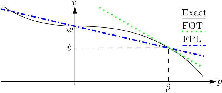
Figure 2: Qualitative interpretation of the FOT and FPL methods.

Some qualitative comparison between the FOT and FPL methods follows (a numerical comparison is provided shortly in Section VII). The FOT method provides the best local linear approximator, and hence it is expected to provide the best approximation accuracy around the linearization point. However, the main downside of the FOT method is its computational complexity. Indeed, solving $(12N)^{2}$ equations with $(12N)^{2}$ variables might not be feasible for large $N$ (i.e., large networks). On the other hand, the FPL method is computationally affordable as it requires only elementary vector-matrix multiplications (provided that ${\bf Y}_{LL}^{-1}$ is precomputed in advance). Moreover, if global behaviour is of interest, it can also provide a better approximation (cf. Figure 2). As a result, the FOT method may be preferable in a slowly time-varying setting whereby the variation of the power injections is relatively small. On the other hand, in the setting of modern distribution networks with high penetration of renewables, the FPL method may be preferable.

Remark 3.

Using methods similar to the previous remarks, the results presented in this section can be straightforwardly adapted to the cases of general multiphase networks and the cases where no phase-to-phase connection exists.

VI Potential Applications

In this section, we briefly discuss the potential applications of our results. As mentioned in the introduction, they can be used to facilitate the development of OPF solvers and real-time control procedures for general multiphase distribution networks. In particular:

• Linear models of Section V can be leveraged to convexify the OPF problem, and thus facilitate the development of OPF-based real-time control techniques. Particularly, the methodology proposed in this paper can be utilized to broaden the applicability of [17, 24, 25, 26] to the case of unbalanced multiphase systems with delta and wye connections.

• Explicit conditions of Theorem 2 can be directly embedded in the optimization problems as convex constraints, thus ensuring existence and non-singularity of the exact high-voltage load-flow solution.

VII Numerical Evaluation

In this section, we evaluate numerically the proposed methodology using IEEE test feeders [27]. Particularly, in the IEEE 37-Bus and 123-Bus networks, we compare our method with the method in [10], which is the classic $Z$-bus method applied to the multiphase setting with disjoint sets of wye- and delta-connected sources. We also use the IEEE 8500-Node test feeder to demonstrate the applicability of the proposed algorithms to a large-scale distribution network.

VII-A An Illustrative Example

We start by demonstrating the proposed methodology and its physical significance using an artificially-designed network. Here, the purpose is to facilitate the understanding and meanwhile provide some intuition.

We consider a balanced network with a single three-phase $PQ$ bus (with index 1) connected to the slack bus via a transmission line. The line admittance matrix is given as follows, in p.u.:

$$\begin{bmatrix}7-12\jmath&-1+2\jmath&-1+2\jmath\\ -1+2\jmath&7-12\jmath&-1+2\jmath\\ -1+2\jmath&-1+2\jmath&7-12\jmath\end{bmatrix}.$$ (20)

Moreover, we assume that the shunt elements are negligible and the vector of slack-bus voltages is ${\bf v}_{0}=(1,e^{-\jmath\frac{2\pi}{3}},e^{\jmath\frac{2\pi}{3}})^{T}$ p.u. Therefore,

$${\bf w}={\bf v}_{0},~{}{\bf Y}_{LL}=\begin{bmatrix}7-12\jmath&-1+2\jmath&-1+2\jmath\\ -1+2\jmath&7-12\jmath&-1+2\jmath\\ -1+2\jmath&-1+2\jmath&7-12\jmath\end{bmatrix}.$$ (21)

Now, exclude the delta connections and let the power injection vector ${\bf s}^{Y}$ be balanced in all phases. As a direct consequence, ${\bf v}_{1}=(v_{1}^{a}){\bf v}_{0}$, which means that the vector of voltages at bus 1 is determined by a scalar $v_{1}^{a}$.

In the left-hand side of Figure 3, we plot the region (a filled circle) in the voltage space where condition (12) holds. It can be seen that this region covers almost all the $v_{1}^{a}$ with a feasible magnitude and an angle between $\pm 35.78^{\circ}$, which is of practical significance. Also, note that the region contains $v_{1}^{a}$ with a magnitude much higher than 1 p.u., which corresponds to the case of strong reverse power flow. In the right-hand side of Figure 3, we take $\widehat{v}_{1}^{a}=1$ p.u. (i.e., $\widehat{{\bf v}}={\bf w}$, $\widehat{{\bf s}}=\mathbf{0}$), ${\bf s}^{Y}=(1.5+0.9\jmath,1.5+0.9\jmath,1.5+0.9\jmath)^{T}$ p.u., and plot the domain $\mathcal{D}_{\rho}(\widehat{{\bf v}})$ projected on $v_{1}^{a}$ for the typical radii $\rho^{\ddagger}(\widehat{{\bf v}},\widehat{{\bf s}})$, $\rho^{\dagger}(\widehat{{\bf v}},\widehat{{\bf s}},{\bf s})$ in (14). We also show the solution $v_{1}^{a}$ in $\mathcal{D}_{\rho}(\widehat{{\bf v}})$ with $\rho=\rho^{\ddagger}(\widehat{{\bf v}},\widehat{{\bf s}})$, where $\widehat{{\bf s}}$ is the power injection corresponding to $\widehat{{\bf v}}$. It can be seen that, when taking the power injections vector ${\bf s}$ into account, the guaranteed solution is localized more accurately using $\mathcal{D}_{\rho}(\widehat{{\bf v}})$ with $\rho=\rho^{\dagger}(\widehat{{\bf v}},\widehat{{\bf s}},{\bf s})$. In Table II, we present the update of ${v_{1}^{a}}^{(k)}$ during the iteration. By observing the third column, it is clear that the iterative update gradually converges. In the fourth column, we give the convergence rate, which is bounded by the contraction modulus $\frac{\xi({\bf s})}{\left(\gamma(\widehat{{\bf v}})-\rho^{\dagger}(\widehat{{\bf v}},\widehat{{\bf s}},{\bf s})\right)^{2}}=0.3264$ (see Appendix for reference).

We note that empirical evidences show that the true convergence rate is usually less than a third of the contraction modulus. As a consequence, when our conditions hold, the iterative method generally reaches a precision of $10^{-6}$ in less than ten iterations.

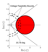
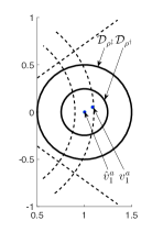
Figure 3: Illustration in voltage space, where the unit of axes is p.u. (Left) The filled red circle represents the set where condition (12) holds, which contains the zero-load point $v_{1}^{a}=1$ (shown as a blue dot); (Right) The set $\mathcal{D}_{\rho}$ (projected onto the space of $v_{1}^{a}$) and the guaranteed solution.

TABLE II: Update of $v_{1}^{a}$ in the iteration. In this table, values are presented with four decimal digits.

$k$	${v_{1}^{a}}^{(k)}$	$|{v_{1}^{a}}^{(k)}-{v_{1}^{a}}^{(k-1)}|$	$\frac{|{v_{1}^{a}}^{(k+1)}-{v_{1}^{a}}^{(k)}|}{|{v_{1}^{a}}^{(k)}-{v_{1}^{a}}^{(k-1)}|}$
$0$	$1.0000+0.0000\jmath$
$1$	$1.0946+0.0531\jmath$	0.1085	0.0990
$2$	$1.0839+0.0526\jmath$	0.0107	0.0912
$3$	$1.0847+0.0531\jmath$	0.0010	0.0921
$4$	$1.0846+0.0531\jmath$	0.0001

VII-B IEEE 37-Bus Feeder

In this example, we evaluate the performance of our method on a network with purely delta connections. Similar to prior works [16, 17, 24, 25, 20], we translate all constant-current and constant-impedance sources in the IEEE data set into constant-power sources. In addition, we fix the voltage regulators in this and all subsequent examples at their default values.

In the original IEEE data set, all sources/loads are delta-connected. Denote this reference power injection vector by $\mathbf{s}^{\mathrm{ref}}$, and let the target power injection be $\mathbf{s}=\kappa\mathbf{s}^{\mathrm{ref}}$ with $\kappa$ as a real number. As there are no mixed wye and delta sources/loads, the conditions on the existence and uniqueness of the load-flow solutions in [10] are also applicable. For comparison, we take the diagonal matrix $\mathbf{\Lambda}$ in [10] to be $\mathbf{W}$, as suggested there. In Figure 4(a), we let $\kappa$ be nonnegative and plot five power intervals. in p.u. Interval 1 contains the power injection $\mathbf{s}$ that satisfies the four conditions in [10]; Interval 2 (resp. 3) shows the injections $\mathbf{s}$ that satisfy the conditions in Theorem 1 (resp. Theorem 2) with $(\widehat{{\bf v}},\widehat{{\bf s}})=({\bf w},\mathbf{0})$. For the rightmost power $\mathbf{s}^{(1)}=3.45\mathbf{s}^{\mathrm{ref}}$, we compute the load-flow solution ${\bf v}^{(1)}$ using iteration (6) (initialized at ${\bf w}$). By choosing this solution ${\bf v}^{(1)}$ and $\mathbf{s}^{(1)}$ as the new $(\widehat{\mathbf{v}},\widehat{\mathbf{s}})$, we obtain Interval 4 (resp. 5) via Theorem 1 (resp. Theorem 2). Note that for this choice of $(\widehat{{\bf v}},\widehat{{\bf s}})$, only some of the power injections in Interval 2 (resp. 3) satisfies the proposed conditions. This is because the conditions guarantee the solution properties only for the power injections in a domain around $\widehat{{\bf s}}$. It can be further shown that, for any power injection vector ${\bf s}$ in the intersection of Interval 2 (resp. 3) and Interval 4 (resp. 5), the guaranteed load-flow solution ${\bf v}$ is consistent. This is because ${\bf v}$ can be computed by iteration (6) initialized at ${\bf v}^{(1)}$.

Numerically, Intervals 1,2, and 3 are the same. However, the complexity of computing Interval 3 is much smaller because of the low computational complexity of verifying conditions (12) and (13). More importantly, Intervals 4 and 5 contain points that are not guaranteed to have the unique solution using the method in [10] – compare to Interval 1. Thus, the proposed method allows for certifying the existence and uniqueness of the load-flow solution for a wider range of power injections.

Next, we evaluate the performance of the two linearization methods proposed in Section V. Figure 4(b) shows the results of the relative errors for both linear models using $\kappa\in[-1.5,1.5]$. As shown, both linear models behave well with relative errors below $1\%$. Moreover, the FOT method has a smaller error around the linearization point whereas the FPL method provides a better global approximation. This corroborates the intuitive illustration in Figure 2. For linear approximations of voltage magnitudes, the errors are at a similar level; hence, for brevity, we do not show them explicitly.

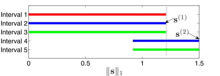
(a) Power intervals (in p.u.) that satisfy conditions on the existence and uniqueness of the load-flow solutions (Intervals 2, 3, 4, and 5) and comparison to the interval obtained by [10] (Interval 1).

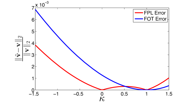
(b) Relative errors in complex load-flow solutions for FOT and FPL methods.

Figure 4: Numerical evaluation for the 37-bus feeder.

VII-C IEEE 123-Bus Feeder

In this section, we consider a larger multiphase network with unbalanced one-, two-, and three-phase sources/loads. This network represents the normal size of many distribution networks in the world. As mentioned in Remark 1, we first delete in matrix ${\bf H}$ the rows that correspond to the lacking phase-to-phase connections and the columns that correspond to the lacking phases.

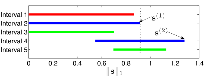
(a) Original injections data. Power intervals (in p.u.) that satisfy conditions on the existence and uniqueness of the load-flow solutions (Intervals 2, 3, 4, and 5) and comparison to the interval obtained by [10] (Interval 1).

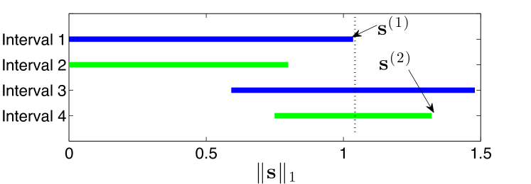
(b) Mixed delta and wye sources. Power intervals (in p.u.) that satisfy conditions on the existence and uniqueness of the load-flow solutions.

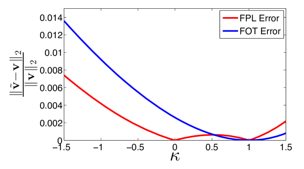
(c) Relative errors in complex load-flow solutions for FOT and FPL methods.

Figure 5: Conditions evaluation for the 123-bus feeder.

Similar to the previous case, let ${\bf s}=\kappa{\bf s}^{\mathrm{ref}}$ with ${\bf s}^{\mathrm{ref}}$ being the reference power injections in this network. Consider then repeating the analysis of the previous subsection. The results are shown in Figures 5(a), with the same interpretation of the intervals as in Figures 4(a). To perform the experiment with mixed delta-wye connections, additional power sources/loads were added to the network, as shown in Table III. In this case of mixed connections, we obtain the intervals of 5(b) in a way similar to the previous analysis. The results match with those obtained in OpenDSS [13], which is the only freely-available solver that works with mixed connections.

TABLE III: Additional Power Sources in 123-Bus Feeder

Bus	Type	Phase-Phase ab	Phase-Phase bc	Phase-Phase ca
		/ Phase a (p.u.)	/ Phase b (p.u.)	/ Phase c (p.u.)
$1$	delta	-0.03-0.01$\jmath$	-0.03-0.01$\jmath$	-0.03-0.01$\jmath$
$35$	wye	-0.02	-0.02	-0.02
$76$	wye	0.04+0.01$\jmath$	0.04+0.01$\jmath$	0.04+0.01$\jmath$
$99$	delta	-0.02-0.01$\jmath$	-0.02-0.01$\jmath$	-0.02-0.01$\jmath$

Finally, in Figure 5(c), we show the results of the relative errors for both linear models using $\kappa\in[-1.5,1.5]$. Here, different from the counterpart in the last section, we have incorporated in ${\bf s}^{\mathrm{ref}}$ the additional sources in Table III. Clearly, the errors vary in a way that is similar to the illustration in Figure 2. In other words, the FPL method provides not only a high computational efficiency but also a better global performance for large distribution networks.

VII-D IEEE 8500-Node Feeder

In this subsection, we illustrate the performance of the proposed methodology using the IEEE 8500-Node feeder [28]. This network represents a large-scale distribution network with detailed modeling of the secondary side of distribution transformers.

In this network, the line-to-line medium-voltage rating is 12.47 kV, and the network contains split-phase secondary loading with line-to-line low-voltage rating of 208 V. In Figure 6, we evaluate the working range of the proposed methodology. In particular, let ${\bf s}=\kappa{\bf s}^{\mathrm{ref}}$ and ${\bf v}$ be the guaranteed load-flow solution that corresponds to ${\bf s}$. Moreover, define the feasibility constraints as $|({\bf v})_{j}|\geq 0.9|({\bf w})_{j}|,\forall j$, where ${\bf w}$ is the zero-load voltage profile given in (4). In this way, $\alpha({\bf v})$ (defined in (8)) becomes both a function of $\|{\bf s}\|_{1}$ and an indicator of the feasibility.

Now, given the knowledge of the zero-load voltage ${\bf w}$, the maximum (in terms of $\ell_{1}$-norm) power vector that satisfies conditions (12) and (13) is ${\bf s}^{(1)}$. Since the conditions are satisfied, we solve for its load-flow solution ${\bf v}^{(1)}$. From the figure, it can be seen that there is already some voltage close to the feasibility boundary. Next, we take the values of $\widehat{{\bf v}}$ (resp. $\widehat{{\bf s}}$) to be ${\bf v}^{(1)}$ (resp. ${\bf s}^{(1)}$). Applying again the proposed conditions, we obtain that the maximum power vector is ${\bf s}^{(2)}$, and the corresponding load-flow solution ${\bf v}^{(2)}$ is obtained. As shown in the figure, some of the voltages in vector ${\bf v}^{(2)}$ are already out of the feasibility region. By taking $\widehat{{\bf v}}$ (resp. $\widehat{{\bf s}}$) to be ${\bf v}^{(2)}$ (resp. ${\bf s}^{(2)}$), we continue the above procedure. Clearly, for this network, some of the voltages drop quickly due to its configuration and the disabled voltage regulators. Because our conditions rely on the voltages, their application becomes more challenging; however, we demonstrate that the conditions can be applied even in the cases where the voltages are significantly below the voltage feasibility boundary.

Finally, in Figure 7, we evaluate the performance of the FPL method for this test feeder. Specifically, we plot the relative error of the phasor approximation using (18) and the corresponding magnitudes approximation using (17), for $\kappa\in[-1,2]$. It can be seen that the relative errors are below $1.4\%$, confirming good scalability of the proposed linear approximation methodology for large-scale distribution networks.

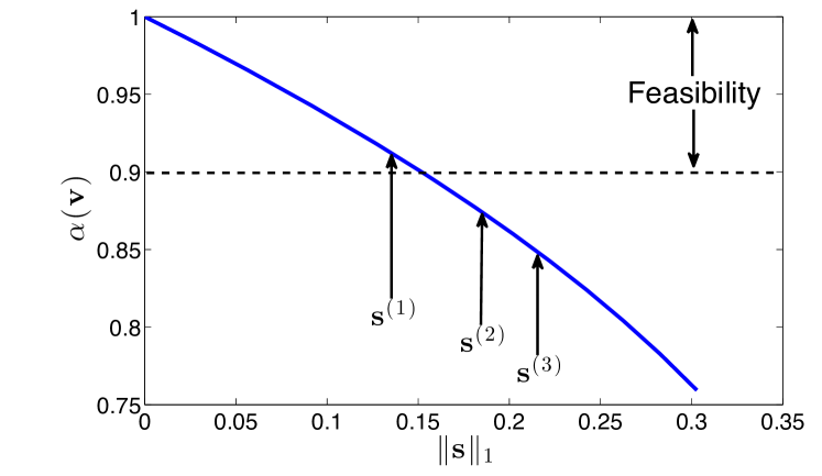
Figure 6: 8500-node test feeder: illustration of the applicability of conditions.

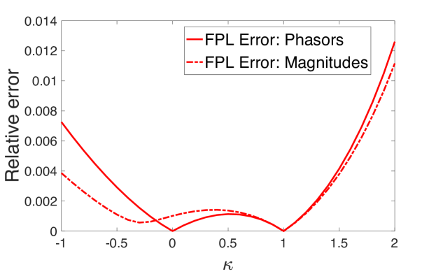
Figure 7: 8500-node test feeder: relative errors in complex load-flow solutions and the corresponding magnitudes approximation for the FPL method.

VII-E Complexity Evaluation

We next analyze the computational complexity of the proposed algorithms. In particular: (i) the verification of conditions (12) and (13) mainly depends on the computation of $\xi(\cdot)$ defined in (7), which has a worst-case complexity of $\mathcal{O}(N^{2})$; (ii) the FPL linear model is essentially a single iteration of (6), which takes $\mathcal{O}(N)$ to complete with LU decomposition in radial networks. To confirm the analysis, we measure the CPU time using MATLAB (on Macbook Pro @3GHz) and gather the results in Table IV. From the second column of Table IV, note that the conditions (12) and (13) can be verified efficiently for 37-Bus and 123-Bus networks, but cannot be verified in real-time for the 8500-Bus network. This adds some restrictiveness in the online applications to very large networks. However, when we pay attention to the third column, the complexity of the FPL method (i.e., single iteration of (6)) scales well with respect to the network size. Recall that, in almost all the experiments, the required number of iterations for accuracy $10^{-6}$ is less than 10. Therefore, the proposed methodology can be very useful in the real-time control and OPF in large networks.

TABLE IV: Complexity Evaluation

Network	Condition (12) and (13)	Single iteration of (6)
$37$-Bus	$2.3$ ms	$0.17$ ms
$123$-Bus	$12$ ms	$0.49$ ms
$8500$-Bus	$76$ s	$51$ ms

VIII Conclusion

The paper extended the classical $Z$-bus load-flow algorithm to general multiphase distribution systems. We derived explicit conditions for the existence of the load-flow solution, and analytically specified a domain in which the solution is unique. These conditions also guarantee the convergence of the load-flow algorithm to this solution. Then, we gave a sufficient condition for the non-singularity of the load-flow Jacobian, and proved that our theoretically guaranteed solution automatically ensures the non-singularity of the load-flow Jacobian. Finally, linear load-flow models were proposed and their approximation accuracy was analyzed. Theoretical results were corroborated through numerical experiments on the IEEE test feeders.

As we have discussed in the paper, the proposed theory and methodology can be leveraged in real-time control and optimal power flow settings; the development of concrete applications in this context is a subject of an ongoing work. We also note that the proposed approach may also be useful in the context of continuation analysis [29, 30, 31], which could be of future research interest. Lastly, the extension of our analysis approach to the case of active voltage regulators and capacitor banks is another future research direction.

-A Proof of Lemma 1

We need to show the three norm axioms. Trivially, note that $\xi(a{\bf s})=|a|\xi({\bf s})$ for any $a\in\mathbb{C}$. Next, the triangle inequality holds because

$$\xi({\bf s}+{\bf s}^{\prime})=\left\|{\bf W}^{-1}{\bf Y}_{LL}^{-1}{\bf W}^{-1}\mathsf{diag}({\bf s}^{Y}+{\bf s}^{\prime Y})\right\|_{\infty}$$

$$\quad+\left\|{\bf W}^{-1}{\bf Y}_{LL}^{-1}{\bf H}^{\textsf{T}}\mathsf{diag}({\bf L}|{\bf w}|)^{-1}\mathsf{diag}({\bf s}^{\Delta}+{\bf s}^{\prime\Delta})\right\|_{\infty}$$

$$=\left\|{\bf W}^{-1}{\bf Y}_{LL}^{-1}{\bf W}^{-1}\mathsf{diag}({\bf s}^{Y})+{\bf W}^{-1}{\bf Y}_{LL}^{-1}{\bf W}^{-1}\mathsf{diag}({\bf s}^{\prime Y})\right\|_{\infty}$$

$$\quad+\Big{\|}{\bf W}^{-1}{\bf Y}_{LL}^{-1}{\bf H}^{\textsf{T}}\mathsf{diag}({\bf L}|{\bf w}|)^{-1}\mathsf{diag}({\bf s}^{\Delta})+$$

$$\quad\quad\quad\quad\quad{\bf W}^{-1}{\bf Y}_{LL}^{-1}{\bf H}^{\textsf{T}}\mathsf{diag}({\bf L}|{\bf w}|)^{-1}\mathsf{diag}({\bf s}^{\prime\Delta})\Big{\|}_{\infty}$$

$$\leq\xi^{Y}({\bf s})+\xi^{Y}({\bf s}^{\prime})+\xi^{\Delta}({\bf s})+\xi^{\Delta}({\bf s}^{\prime})=\xi({\bf s})+\xi({\bf s}^{\prime}),$$

where the inequality follows by the triangle inequality for the induced matrix norm. Finally, if $\xi({\bf s})=0$, it necessarily holds that ${\bf W}^{-1}{\bf Y}_{LL}^{-1}{\bf W}^{-1}\mathsf{diag}({\bf s}^{Y})$ and ${\bf W}^{-1}{\bf Y}_{LL}^{-1}{\bf H}^{\textsf{T}}\mathsf{diag}({\bf L}|{\bf w}|)^{-1}\mathsf{diag}({\bf s}^{\Delta})$ are zero matrices. This necessarily implies that ${\bf s}^{Y}$ and ${\bf s}^{\Delta}$ are zero vectors.

-B Proof of Theorem 1

For the purpose of the proof, we find it convenient to re-parametrize using ${\bf u}:={\bf W}^{-1}{\bf v}$. Then, (4) is equivalent to

$${\bf u}=\widetilde{\mathbf{G}}_{{\bf s}^{Y}{\bf s}^{\Delta}}({\bf u}) ={\bf 1}+{\bf W}^{-1}{\bf Y}_{LL}^{-1}\overline{{\bf W}}^{-1}\mathsf{diag}(\overline{{\bf u}})^{-1}\overline{{\bf s}^{Y}}$$

$$\,+{\bf W}^{-1}{\bf Y}_{LL}^{-1}{\bf H}^{\textsf{T}}\mathsf{diag}\left({\bf H}\overline{{\bf W}}\overline{{\bf u}}\right)^{-1}\overline{{\bf s}^{\Delta}}.$$ (22)

As ${\bf W}$ defines an invertible relationship between ${\bf v}$ and ${\bf u}$, we next focus on the solution properties of (-B). By the Banach fixed-point theorem, what we need to show is that $\widetilde{\mathbf{G}}_{{\bf s}^{Y}{\bf s}^{\Delta}}({\bf u})$ is a self-mapping and contraction mapping on

$$\widetilde{\mathcal{D}}_{\rho}(\widehat{{\bf u}}):=\{{\bf u}:\,|({\bf u})_{j}-(\widehat{{\bf u}})_{j}|\leq\rho,\,j=1\ldots 3N\}$$ (23)

for some $\rho\in(0,\gamma(\widehat{{\bf v}}))$ that satisfies (9) and (10).

-B1 Proof of Self-Mapping

The goal here is to show that, for $\rho\in(0,\gamma(\widehat{{\bf v}}))$ fulfilling (9), $\|{\bf u}^{(k)}-\widehat{{\bf u}}\|_{\infty}\leq\rho$ leads to $\|{\bf u}^{(k+1)}-\widehat{{\bf u}}\|_{\infty}\leq\rho$.

By definition, we have

$$\mathbf{u}^{(k+1)}-\widehat{\mathbf{u}}$$

$$=\mathbf{W}^{-1}\mathbf{Y}_{LL}^{-1}\overline{\mathbf{W}}^{-1}\left(\mathsf{diag}(\overline{\mathbf{u}}^{(k)})^{-1}\overline{\mathbf{s}^{Y}}-\mathsf{diag}(\overline{\widehat{\mathbf{u}}})^{-1}\overline{\widehat{\mathbf{s}}^{Y}}\right)$$

$$+\mathbf{W}^{-1}\mathbf{Y}_{LL}^{-1}\mathbf{H}^{T}\left(\mathsf{diag}(\mathbf{H}\overline{\mathbf{W}}\overline{\mathbf{u}}^{(k)})^{-1}\overline{\mathbf{s}^{\Delta}}-\mathsf{diag}(\mathbf{H}\overline{\mathbf{W}}\overline{\widehat{\mathbf{u}}})^{-1}\overline{\widehat{\mathbf{s}}^{\Delta}}\right)$$

$$=\mathbf{W}^{-1}\mathbf{Y}_{LL}^{-1}\overline{\mathbf{W}}^{-1}\left(\mathsf{diag}(\overline{\mathbf{u}}^{(k)})^{-1}\overline{\mathbf{s}^{Y}}-\mathsf{diag}(\overline{\mathbf{u}}^{(k)})^{-1}\overline{\widehat{\mathbf{s}}^{Y}}\right)$$

$$+\mathbf{W}^{-1}\mathbf{Y}_{LL}^{-1}\overline{\mathbf{W}}^{-1}\left(\mathsf{diag}(\overline{\mathbf{u}}^{(k)})^{-1}\overline{\widehat{\mathbf{s}}^{Y}}-\mathsf{diag}(\overline{\widehat{\mathbf{u}}})^{-1}\overline{\widehat{\mathbf{s}}^{Y}}\right)$$

$$+\mathbf{W}^{-1}\mathbf{Y}_{LL}^{-1}\mathbf{H}^{T}\left(\mathsf{diag}(\mathbf{H}\overline{\mathbf{W}}\overline{\mathbf{u}}^{(k)})^{-1}\overline{\mathbf{s}^{\Delta}}-\mathsf{diag}(\mathbf{H}\overline{\mathbf{W}}\overline{\mathbf{u}}^{(k)})^{-1}\overline{\widehat{\mathbf{s}}^{\Delta}}\right)$$

$$+\mathbf{W}^{-1}\mathbf{Y}_{LL}^{-1}\mathbf{H}^{T}\left(\mathsf{diag}(\mathbf{H}\overline{\mathbf{W}}\overline{\mathbf{u}}^{(k)})^{-1}\overline{\widehat{\mathbf{s}}^{\Delta}}-\mathsf{diag}(\mathbf{H}\overline{\mathbf{W}}\overline{\widehat{\mathbf{u}}})^{-1}\overline{\widehat{\mathbf{s}}^{\Delta}}\right).$$ (24)

We can rearrange the right-hand side of (-B1) as follows. For example, for the second term, we have

$$\mathbf{W}^{-1}\mathbf{Y}_{LL}^{-1}\overline{\mathbf{W}}^{-1}\left(\mathsf{diag}(\overline{\mathbf{u}}^{(k)})^{-1}\overline{\widehat{\mathbf{s}}^{Y}}-\mathsf{diag}(\overline{\widehat{\mathbf{u}}})^{-1}\overline{\widehat{\mathbf{s}}^{Y}}\right)$$

$$=-{\bf W}^{-1}\mathbf{Y}_{LL}^{-1}\overline{{\bf W}}^{-1}\mathsf{diag}(\overline{\widehat{{\bf s}}^{Y}})\begin{bmatrix}\displaystyle\frac{(\overline{{\bf u}}^{(k)})_{1}-(\overline{\widehat{{\bf u}}})_{1}}{(\overline{{\bf u}}^{(k)})_{1}(\overline{\widehat{{\bf u}}})_{1}}\ldots\displaystyle\frac{(\overline{{\bf u}}^{(k)})_{3N}-(\overline{\widehat{{\bf u}}})_{3N}}{(\overline{{\bf u}}^{(k)})_{3N}(\overline{\widehat{{\bf u}}})_{3N}}\end{bmatrix}^{\textsf{T}}$$ (25)

Similar rearrangements can be applied to the remaining terms in (-B1). Therefore, by triangular inequality, the definition of the induced matrix norm, and definition (7), it holds that

$$\|\mathbf{u}^{(k+1)}-\widehat{\mathbf{u}}\|_{\infty}\leq\xi^{Y}({\bf s}-\widehat{{\bf s}})\max\limits_{j\in\{1,...,3N\}}\displaystyle\left(1/|({\bf u}^{(k)})_{j}|\right)$$

$$+\xi^{Y}(\widehat{{\bf s}})\max\limits_{j\in\{1,...,3N\}}\displaystyle\left(|({\bf u}^{(k)})_{j}-(\widehat{{\bf u}})_{j}|/[|({\bf u}^{(k)})_{j}||(\widehat{{\bf u}})_{j}|]\right)$$

$$+\xi^{\Delta}({\bf s}-\widehat{{\bf s}})\max\limits_{j\in\{1,...,3N\}}\displaystyle\left(1\middle/\displaystyle\frac{|({\bf H}{\bf W}{\bf u}^{(k)})_{j}|}{({\bf L}|{\bf w}|)_{j}}\right)$$

$$+\xi^{\Delta}(\widehat{{\bf s}})\max\limits_{j\in\{1,...,3N\}}\displaystyle\displaystyle\frac{|({\bf H}{\bf W}{\bf u}^{(k)})_{j}-({\bf H}{\bf W}\widehat{{\bf u}})_{j}|/({\bf L}|{\bf w}|)_{j}}{\displaystyle\frac{|({\bf H}{\bf W}{\bf u}^{(k)})_{j}|}{({\bf L}|{\bf w}|)_{j}}\displaystyle\frac{|({\bf H}{\bf W}\widehat{{\bf u}})_{j}|}{({\bf L}|{\bf w}|)_{j}}}.$$ (26)

Observe that the following is true for any $j\in\{1,...,3N\}$ whenever $\|{\bf u}^{(k)}-\widehat{{\bf u}}\|\leq\rho$:

$$|({\bf u}^{(k)})_{j}|\geq|(\widehat{{\bf u}})_{j}|-|({\bf u}^{(k)})_{j}-(\widehat{{\bf u}})_{j}|\geq\alpha(\widehat{{\bf v}})-\rho$$ (27a)

$$|({\bf H}{\bf W}{\bf u}^{(k)})_{j}-({\bf H}{\bf W}\widehat{{\bf u}})_{j}|\leq({\bf L}|{\bf w}|)_{j}\rho$$ (27b)

$$|({\bf H}{\bf W}{\bf u}^{(k)})_{j}|\geq(\beta(\widehat{{\bf v}})-\rho)({\bf L}|{\bf w}|)_{j},$$ (27c)

where $\alpha(\cdot)$ and $\beta(\cdot)$ are defined in (8). In details, (27b) holds because

$$|({\bf H}{\bf W}{\bf u}^{(k)})_{j}-({\bf H}{\bf W}\widehat{{\bf u}})_{j}|$$

$$=\left|\left(({\bf w})_{\ell}({\bf u}^{(k)})_{\ell}-({\bf w})_{\ell^{\prime}}({\bf u}^{(k)})_{\ell^{\prime}}\right)-\left(({\bf w})_{\ell}(\widehat{{\bf u}})_{\ell}-({\bf w})_{\ell^{\prime}}(\widehat{{\bf u}})_{\ell^{\prime}}\right)\right|$$

$$\leq|({\bf w})_{\ell}|\left|({\bf u}^{(k)})_{\ell}-(\widehat{{\bf u}})_{\ell}\right|+|({\bf w})_{\ell^{\prime}}|\left|({\bf u}^{(k)})_{\ell^{\prime}}-(\widehat{{\bf u}})_{\ell^{\prime}}\right|$$

$$\leq\left(|({\bf w})_{\ell}|+|({\bf w})_{\ell^{\prime}}|\right)\|{\bf u}^{(k)}-\widehat{{\bf u}}\|_{\infty}\leq({\bf L}|{\bf w}|)_{j}\rho$$ (28)

for some $\ell,\ell^{\prime}$ in $\{1,...,3N\}$, and (27c) holds because

$$|({\bf H}{\bf W}{\bf u}^{(k)})_{j}|\geq|({\bf H}{\bf W}\widehat{{\bf u}})_{j}|-|({\bf H}{\bf W}{\bf u}^{(k)})_{j}-({\bf H}{\bf W}\widehat{{\bf u}})_{j}|$$

$$\geq(\beta(\widehat{{\bf v}})-\rho)({\bf L}|{\bf w}|)_{j}.$$ (29)

In this way, for $\rho\in(0,\gamma(\widehat{{\bf v}}))$, we obtain

$$\|\mathbf{u}^{(k+1)}-\widehat{\mathbf{u}}\|_{\infty}$$

$$\leq\frac{\xi^{Y}(\mathbf{s}-\widehat{\mathbf{s}})+\displaystyle\rho\xi^{Y}(\widehat{\mathbf{s}})/\alpha(\widehat{{\bf v}})}{\alpha(\widehat{{\bf v}})-\rho}+\frac{\xi^{\Delta}(\mathbf{s}-\widehat{\mathbf{s}})+\displaystyle\rho\xi^{\Delta}(\widehat{\mathbf{s}})/\beta(\widehat{{\bf v}})}{\beta(\widehat{{\bf v}})-\rho}.$$ (30)

This implies that $\|{\bf u}^{(k)}-\widehat{{\bf u}}\|_{\infty}\leq\rho$ gives $\|{\bf u}^{(k+1)}-\widehat{{\bf u}}\|_{\infty}\leq\rho$ for $\rho\in(0,\gamma(\widehat{{\bf v}}))$ fulfilling (9), and hence completes the proof.

-B2 Proof of Contraction

In this part, assuming there is a $\rho\in(0,\gamma(\widehat{{\bf v}}))$ fulfilling (9), we prove that $\|{\bf u}^{(k+1)}-{\bf u}^{(k)}\|_{\infty}<\|{\bf u}^{(k)}-{\bf u}^{(k-1)}\|_{\infty}$ if $\rho$ further satisfies (10).

Similar to the proof of self-mapping, we have

$$\mathbf{u}^{(k+1)}-\mathbf{u}^{(k)}$$

$$=\mathbf{W}^{-1}\mathbf{Y}_{LL}^{-1}\overline{\mathbf{W}}^{-1}\left(\mathsf{diag}(\overline{\mathbf{u}}^{(k)})^{-1}\overline{\mathbf{s}^{\mathbf{Y}}}-\mathsf{diag}(\overline{\mathbf{u}}^{(k-1)})^{-1}\overline{\mathbf{s}^{\mathbf{Y}}}\right)$$

$$+\mathbf{W}^{-1}\mathbf{Y}_{LL}^{-1}\mathbf{H}^{T}\left(\mathsf{diag}(\mathbf{H}\overline{\mathbf{W}}\overline{\mathbf{u}}^{(k)})^{-1}\overline{\mathbf{s}^{\Delta}}-\mathsf{diag}(\mathbf{H}\overline{\mathbf{W}}\overline{\mathbf{u}}^{(k-1)})^{-1}\overline{\mathbf{s}^{\Delta}}\right).$$

Then, via derivations analogues to (-B1) and (27), there is

$$\|\mathbf{u}^{(k+1)}-\mathbf{u}^{(k)}\|_{\infty}$$

$$\leq\xi^{Y}({\bf s})\max\limits_{j\in\{1,\ldots,3N\}}\displaystyle|({\bf u}^{(k)})_{j}-({\bf u}^{(k-1)})_{j}|/[|({\bf u}^{(k)})_{j}||({\bf u}^{(k-1)})_{j}|]$$

$$+\xi^{\Delta}({\bf s})\max\limits_{j\in\{1,...,3N\}}\displaystyle\frac{\displaystyle|({\bf H}{\bf W}{\bf u}^{(k)})_{j}-({\bf H}{\bf W}{\bf u}^{(k-1)})_{j}|/({\bf L}|{\bf w}|)_{j}}{\displaystyle\frac{|({\bf H}{\bf W}{\bf u}^{(k)})_{j}|}{({\bf L}|{\bf w}|)_{j}}\displaystyle\frac{|({\bf H}{\bf W}{\bf u}^{(k-1)})_{j}|}{({\bf L}|{\bf w}|)_{j}}}$$

$$\leq\left(\frac{\xi^{Y}(\mathbf{s})}{(\alpha(\widehat{{\bf v}})-\rho)^{2}}+\frac{\xi^{\Delta}(\mathbf{s})}{(\beta(\widehat{{\bf v}})-\rho)^{2}}\right)\|\mathbf{u}^{(k)}-\mathbf{u}^{(k-1)}\|_{\infty}.$$ (31)

Clearly, $\|{\bf u}^{(k+1)}-{\bf u}^{(k)}\|_{\infty}<\|{\bf u}^{(k)}-{\bf u}^{(k-1)}\|_{\infty}$ if $\rho$ further satisfies (10).

-C Proof of Theorem 2

For item (i), we first note that because the Jacobian ${\bf J}$ associated with the mapping ${\bf h}$ in (5) is a square matrix, the existence and uniqueness of the solution to the set of linear equations ${\bf J}\frac{\partial{\bf y}}{\partial{\bf x}}={\bf I}_{12N}$ is equivalent to the invertibility of ${\bf J}$. In such case, the solution is given by $\frac{\partial{\bf y}}{\partial{\bf x}}={\bf J}^{-1}$. Therefore, we can analyze the invertibility of ${\bf J}$ by analyzing the set of equations (16). In particular, we next show that if (12) is satisfied, (16) has a unique solution. Because the system is linear with respect to the rectangular coordinates and there are as many unknowns as equations, the result is equivalent to showing that the corresponding homogeneous system of equations has only the trivial solution (see, e.g., [32]). Note that the homogeneous system is the same for every column of (16) and is given by

$$\mathsf{diag}\left({\bf H}^{\textsf{T}}\overline{{\bf i}^{\Delta}}\right){\mbox{\boldmath$\Delta$}}_{V}+\mathsf{diag}({\bf v}){\bf H}^{\textsf{T}}\overline{{\mbox{\boldmath$\Delta$}}}_{I},$$

$$\quad=\mathsf{diag}({\bf v})\overline{{\bf Y}}_{LL}\overline{{\mbox{\boldmath$\Delta$}}}_{V}+\mathsf{diag}(\overline{{\bf Y}}_{L0}\overline{{\bf v}}_{0}+\overline{{\bf Y}}_{LL}\overline{{\bf v}}){\mbox{\boldmath$\Delta$}}_{V}$$ (32a)

$${\bf 0}=\mathsf{diag}\left({\bf H}{\bf v}\right)\overline{{\mbox{\boldmath$\Delta$}}}_{I}+\mathsf{diag}(\overline{{\bf i}^{\Delta}}){\bf H}{\mbox{\boldmath$\Delta$}}_{V},$$ (32b)

where ${\mbox{\boldmath$\Delta$}}_{V},{\mbox{\boldmath$\Delta$}}_{I}$ are solution vectors.

Assume, by the way of contradiction, that there exists a solution ${\mbox{\boldmath$\Delta$}}^{\prime}:=({{\mbox{\boldmath$\Delta$}}^{\prime}}_{V}^{\textsf{T}},{{\mbox{\boldmath$\Delta$}}^{\prime}}_{I}^{\textsf{T}})^{\textsf{T}}$ to (32) such that ${\mbox{\boldmath$\Delta$}}^{\prime}\neq 0$. In particular, any vector ${\mbox{\boldmath$\Delta$}}^{\epsilon}:=\epsilon{\mbox{\boldmath$\Delta$}}^{\prime}$ for $\epsilon>0$ is a solution to (32).

Now consider two power networks with the same topology but different voltages and between-phase currents. In particular, let ${\bf v}_{1}^{\epsilon}={\bf v}+{\mbox{\boldmath$\Delta$}}^{\epsilon}_{V}$, ${\bf i}^{\epsilon,\Delta}_{1}={\bf i}^{\Delta}+{\mbox{\boldmath$\Delta$}}_{I}^{\epsilon}$, ${\bf v}_{2}^{\epsilon}={\bf v}-{\mbox{\boldmath$\Delta$}}^{\epsilon}_{V}$, and ${\bf i}^{\epsilon,\Delta}_{2}={\bf i}^{\Delta}-{\mbox{\boldmath$\Delta$}}_{I}^{\epsilon}$, while ${\bf v}_{0}$ is the same in both networks. Note that there exists $\epsilon_{1}>0$ such that for all $\epsilon<\epsilon_{1}$, ${\bf v}_{1}^{\epsilon},{\bf v}_{2}^{\epsilon}\in{\cal D}_{\rho^{\dagger}}({\bf v})$, where ${\cal D}_{\rho^{\dagger}}$ is defined in (11) (with $\widehat{{\bf v}}={\bf v}$).

Let ${\bf s}_{1}^{\epsilon,Y},{\bf s}_{1}^{\epsilon,\Delta},{\bf s}_{2}^{\epsilon,Y},{\bf s}_{2}^{\epsilon,\Delta}$ be the corresponding power injections. Using (1), we obtain that

$${\bf s}_{1}^{\epsilon,Y}-{\bf s}_{2}^{\epsilon,Y}=2\Big{(}\mathsf{diag}({\bf v})\overline{{\bf Y}}_{LL}\overline{{\mbox{\boldmath$\Delta$}}}^{\epsilon}_{V}$$

$$\quad+\mathsf{diag}(\overline{{\bf Y}}_{L0}\overline{{\bf v}}_{0}+\overline{{\bf Y}}_{LL}\overline{{\bf v}}){\mbox{\boldmath$\Delta$}}^{\epsilon}_{V}-\mathsf{diag}\left({\bf H}^{\textsf{T}}\overline{{\bf i}^{\Delta}}\right){\mbox{\boldmath$\Delta$}}^{\epsilon}_{V}$$

$$\quad-\mathsf{diag}({\bf v}){\bf H}^{\textsf{T}}\overline{{\mbox{\boldmath$\Delta$}}}^{\epsilon}_{I}\Big{)},$$

$${\bf s}_{1}^{\epsilon,\Delta}-{\bf s}_{2}^{\epsilon,\Delta}=2\left(\mathsf{diag}\left({\bf H}{\bf v}\right)\overline{{\mbox{\boldmath$\Delta$}}}^{\epsilon}_{I}+\mathsf{diag}(\overline{{\bf i}^{\Delta}}){\bf H}{\mbox{\boldmath$\Delta$}}^{\epsilon}_{V}\right),$$

which by (32) implies that ${\bf s}_{1}^{\epsilon,Y}={\bf s}_{2}^{\epsilon,Y}$ and ${\bf s}_{1}^{\epsilon,\Delta}={\bf s}_{2}^{\epsilon,\Delta}.$

Let ${\bf s}^{\epsilon}:=(({\bf s}_{1}^{\epsilon,Y})^{\textsf{T}},({\bf s}_{1}^{\epsilon,\Delta})^{\textsf{T}})^{\textsf{T}}$. It is easy to see that there exists $\epsilon_{2}>0$ such that for all $\epsilon<\epsilon_{2}$, ${\bf s}^{\epsilon}$ satisfies (13) (with $\widehat{{\bf s}}={\bf s}$). Let $\epsilon^{*}=\min\{\epsilon_{1},\epsilon_{2}\}$. Then, by Theorem 2, we have that for any $\epsilon\in(0,\epsilon^{*})$, ${\bf v}^{\epsilon}_{1}={\bf v}^{\epsilon}_{2}$ and ${\bf i}^{\epsilon,\Delta}_{1}={\bf i}^{\epsilon,\Delta}_{2}$. This is equivalent to having ${\mbox{\boldmath$\Delta$}}_{V}^{\epsilon}={\bf 0}$ and ${\mbox{\boldmath$\Delta$}}_{I}^{\epsilon}={\bf 0}$, which is a contradiction to our assumption that ${\mbox{\boldmath$\Delta$}}^{\epsilon}\neq 0$. This completes the proof of item (i).

For items (ii)-(iv) in the theorem, we show that conditions (12) and (13) imply conditions (9) and (10) of Theorem 1. From the proof of Lemma 1 in [8], whenever (12) and (13) are satisfied, we have

$$\rho^{2}-\rho((\gamma(\widehat{{\bf v}}))^{2}-\xi(\widehat{{\bf s}}))/\gamma(\widehat{{\bf v}})+\xi({\bf s}-\widehat{{\bf s}})\leq 0$$ (33)

for $\rho\in[\rho^{\dagger}(\widehat{{\bf v}},\widehat{{\bf s}},{\bf s}),\rho^{\ddagger}(\widehat{{\bf v}},\widehat{{\bf s}})]\subseteq(0,\gamma(\widehat{{\bf v}}))$. After re-organization, the above inequality becomes

$$\frac{\xi({\bf s}-\widehat{{\bf s}})+\displaystyle\rho\xi(\widehat{{\bf s}})/\gamma(\widehat{{\bf v}})}{\gamma(\widehat{{\bf v}})-\rho}\leq\rho.$$ (34)

Note that

$$\frac{\xi^{Y}(\mathbf{s}-\widehat{\mathbf{s}})+\displaystyle\frac{\xi^{Y}(\widehat{\mathbf{s}})}{\alpha(\widehat{{\bf v}})}\rho}{\alpha(\widehat{{\bf v}})-\rho}+\frac{\xi^{\Delta}(\mathbf{s}-\widehat{\mathbf{s}})+\displaystyle\frac{\xi^{\Delta}(\widehat{\mathbf{s}})}{\beta(\widehat{{\bf v}})}\rho}{\beta(\widehat{{\bf v}})-\rho}\leq\displaystyle\frac{\xi({\bf s}-\widehat{{\bf s}})+\displaystyle\frac{\xi(\widehat{{\bf s}})}{\gamma(\widehat{{\bf v}})}\rho}{\gamma(\widehat{{\bf v}})-\rho},$$ (35)

and hence (9) is satisfied. Namely, $\widetilde{\mathbf{G}}_{{\bf s}^{Y}{\bf s}^{\Delta}}({\bf u})$ is a self-mapping on domain $\widetilde{\mathcal{D}}_{\rho}(\widehat{{\bf u}})$ for $\rho\in[\rho^{\dagger}(\widehat{{\bf v}},\widehat{{\bf s}},{\bf s}),\rho^{\ddagger}(\widehat{{\bf v}},\widehat{{\bf s}})]$.

Further, taking into account (13) and the fact that $\xi(\cdot)$ is a norm (cf. Lemma 1), we have

$$\xi({\bf s}) \leq\xi({\bf s}-\widehat{{\bf s}})+\xi(\widehat{{\bf s}})<\frac{1}{4}\left(\frac{(\gamma(\widehat{{\bf v}}))^{2}-\xi(\widehat{{\bf s}})}{\gamma(\widehat{{\bf v}})}\right)^{2}+\xi(\widehat{{\bf s}})$$

$$=\frac{1}{4}\left(\frac{(\gamma(\widehat{{\bf v}}))^{2}+\xi(\widehat{{\bf s}})}{\gamma(\widehat{{\bf v}})}\right)^{2}=(\gamma(\widehat{{\bf v}})-\rho^{\ddagger}(\widehat{{\bf v}},\widehat{{\bf s}}))^{2}.$$ (36)

Then, it is easy to see that

$$\frac{\xi^{Y}(\mathbf{s})}{(\alpha(\widehat{{\bf v}})-\rho)^{2}}+\frac{\xi^{\Delta}(\mathbf{s})}{(\beta(\widehat{{\bf v}})-\rho)^{2}}\leq\displaystyle\frac{\xi({\bf s})}{\left(\gamma(\widehat{{\bf v}})-\rho\right)^{2}}<\displaystyle\frac{\left(\gamma(\widehat{{\bf v}})-\rho^{\ddagger}(\widehat{{\bf v}},\widehat{{\bf s}})\right)^{2}}{\left(\gamma(\widehat{{\bf v}})-\rho\right)^{2}}\leq 1$$

for $\rho\in[\rho^{\dagger}(\widehat{{\bf v}},\widehat{{\bf s}},{\bf s}),\rho^{\ddagger}(\widehat{{\bf v}},\widehat{{\bf s}})]$. It implies that $\widetilde{\mathbf{G}}_{{\bf s}^{Y}{\bf s}^{\Delta}}({\bf u})$ is also a contraction mapping on $\widetilde{\mathcal{D}}_{\rho}(\widehat{{\bf u}})$ with $\rho\in[\rho^{\dagger}(\widehat{{\bf v}},\widehat{{\bf s}},{\bf s}),\rho^{\ddagger}(\widehat{{\bf v}},\widehat{{\bf s}})]$. This completes the proof of items (ii)-(iv).

For item (v), we derive as follows. First, by (8) and the bound of (27a), there is

$$\gamma(\widehat{{\bf v}})-\rho^{\ddagger}(\widehat{{\bf v}},\widehat{{\bf s}})\leq\alpha(\widehat{{\bf v}})-\rho^{\ddagger}(\widehat{{\bf v}},\widehat{{\bf s}})\leq\alpha({\bf v}).$$ (37)

Then, by the bound of (27c), we have

$$\gamma(\widehat{{\bf v}})-\rho^{\ddagger}(\widehat{{\bf v}},\widehat{{\bf s}})\leq\beta(\widehat{{\bf v}})-\rho^{\ddagger}(\widehat{{\bf v}},\widehat{{\bf s}})\leq\beta({\bf v}).$$ (38)

Combination of (37) and (38) yields

$$\gamma(\widehat{{\bf v}})-\rho^{\ddagger}(\widehat{{\bf v}},\widehat{{\bf s}})\leq\gamma({\bf v}).$$ (39)

Therefore, by (-C), we have

$$\xi({\bf s})<(\gamma(\widehat{{\bf v}})-\rho^{\ddagger}(\widehat{{\bf v}},\widehat{{\bf s}}))^{2}\leq(\gamma({\bf v}))^{2}$$ (40)

and hereby complete the proof.

-D Proof of Theorem 3

Note that (18) is in fact a single iteration of the fixed-point equation initialized at $\widehat{{\bf v}}$. Therefore, by identifying ${\bf v}^{(0)}=\widehat{{\bf v}}$ and ${\bf v}^{(1)}=\widetilde{{\bf v}}$, we have that

$$\|\widetilde{{\bf v}}-{\bf v}\|_{\infty}\leq q\|\widehat{{\bf v}}-{\bf v}\|_{\infty} \leq q\|{\bf w}\|_{\infty}\|\widehat{{\bf u}}-{\bf u}\|_{\infty}\leq q\|{\bf w}\|_{\infty}\rho^{\dagger},$$

where $q<1$ is the contraction coefficient given in the proof of Theorem 2 – cf. (-B2); the first inequality follows by the Banach fixed point theorem; the second inequality holds by definition of ${\bf v}={\bf W}{\bf u}$; and the last inequality follows because ${\bf v}\in{\cal D}_{\rho^{\dagger}}(\widehat{{\bf v}})$ (cf. (11)).

References

• [1] W. H. Kersting, Distribution System Modeling and Analysis.   2nd ed., Boca Raton, FL: CRC Press, 2007.
• [2] Y. Wang and W. Xu, “The existence of multiple power flow solutions in unbalanced three-phase circuits,” IEEE Transactions on Power Systems, vol. 18, no. 2, pp. 605–610, May 2003.
• [3] B. K. Johnson, “Extraneous and false load flow solutions,” IEEE Transactions on Power Apparatus and Systems, vol. 96, no. 2, pp. 524–534, 1977.
• [4] H. D. Nguyen and K. S. Turitsyn, “Appearance of multiple stable load flow solutions under power flow reversal conditions,” in 2014 IEEE PES General Meeting — Conference Exposition, 2014, pp. 1–5.
• [5] J. W. Simpson-Porco, “A Theory of Solvability for Lossless Power Flow Equations – Part I: Fixed-Point Power Flow,” IEEE Transactions on Control of Network Systems, vol. PP, no. 99, pp. 1–1, 2017.
• [6] S. Bolognani and S. Zampieri, “On the existence and linear approximation of the power flow solution in power distribution networks,” IEEE Transactions on Power Systems, vol. 31, no. 1, pp. 163–172, Jan 2016.
• [7] S. Yu, H. D. Nguyen, and K. S. Turitsyn, “Simple certificate of solvability of power flow equations for distribution systems,” in 2015 IEEE Power Energy Society General Meeting, 2015, pp. 1–5.
• [8] C. Wang, A. Bernstein, J.-Y. Le Boudec, and M. Paolone, “Explicit Conditions on Existence and Uniqueness of Load-Flow Solutions in Distribution Networks,” IEEE Transactions on Smart Grid, vol. PP, no. 99, pp. 1–1, 2016.
• [9] C. Wang, A. Bernstein, J. Y. L. Boudec, and M. Paolone, “Existence and uniqueness of load-flow solutions in three-phase distribution networks,” IEEE Transactions on Power Systems, vol. 32, no. 4, pp. 3319–3320, July 2017.
• [10] M. Bazrafshan and N. Gatsis, “Convergence of the Z-Bus Method for Three-Phase Distribution Load-Flow with ZIP Loads,” IEEE Transactions on Power Systems, vol. PP, no. 99, pp. 1–1, 2017.
• [11] T. H. Chen, M. S. Chen, K. J. Hwang, P. Kotas, and E. A. Chebli, “Distribution system power flow analysis-a rigid approach,” IEEE Transactions on Power Delivery, vol. 6, no. 3, pp. 1146–1152, Jul 1991.
• [12] D. Borzacchiello, F. Chinesta, M. Malik, R. García-Blanco, and P. Diez, “Unified formulation of a family of iterative solvers for power systems analysis,” Electric Power Systems Research, vol. 140, pp. 201 – 208, 2016.
• [13] R. C. Dugan and T. E. McDermott, “An open source platform for collaborating on smart grid research,” in 2011 IEEE Power and Energy Society General Meeting, July 2011, pp. 1–7.
• [14] Electric Power Research Institute (EPRI), “OpenDSS Solution Technique,” [Online] Available at: https://sourceforge.net/p/electricdss/code/HEAD/tree/trunk/Distrib/Doc/.
• [15] I. Kocar, J. Mahseredjian, U. Karaagac, G. Soykan, and O. Saad, “Multiphase load-flow solution for large-scale distribution systems using mana,” IEEE Transactions on Power Delivery, vol. 29, no. 2, pp. 908–915, April 2014.
• [16] S. H. Low, “Convex relaxation of optimal power flow – part I: Formulations and equivalence,” IEEE Transactions on Control of Network Systems, vol. 1, no. 1, pp. 15–27, March 2014.
• [17] S. S. Guggilam, E. Dall’Anese, Y. C. Chen, S. V. Dhople, and G. B. Giannakis, “Scalable optimization methods for distribution networks with high pv integration,” IEEE Transactions on Smart Grid, vol. 7, no. 4, pp. 2061–2070, July 2016.
• [18] K. Christakou, J.-Y. Le Boudec, M. Paolone, and D.-C. Tomozei, “Efficient Computation of Sensitivity Coefficients of Node Voltages and Line Currents in Unbalanced Radial Electrical Distribution Networks,” IEEE Transactions on Smart Grid, vol. 4, no. 2, pp. 741–750, 2013.
• [19] S. V. Dhople, S. S. Guggilam, and Y. C. Chen, “Linear approximations to ac power flow in rectangular coordinates,” in 2015 53rd Annual Allerton Conference on Communication, Control, and Computing (Allerton), Sept 2015, pp. 211–217.
• [20] S. Bolognani and F. Dörfler, “Fast power system analysis via implicit linearization of the power flow manifold,” in 2015 53rd Annual Allerton Conference on Communication, Control, and Computing (Allerton), Sept 2015, pp. 402–409.
• [21] A. Garces, “A linear three-phase load flow for power distribution systems,” IEEE Transactions on Power Systems, vol. 31, no. 1, pp. 827–828, Jan 2016.
• [22] H. Ahmadi, J. R. Martı´, and A. von Meier, “A linear power flow formulation for three-phase distribution systems,” IEEE Transactions on Power Systems, vol. 31, no. 6, pp. 5012–5021, Nov 2016.
• [23] V. Kekatos, L. Zhang, G. B. Giannakis, and R. Baldick, “Voltage regulation algorithms for multiphase power distribution grids,” IEEE Transactions on Power Systems, vol. 31, no. 5, pp. 3913–3923, Sept 2016.
• [24] A. Bernstein, L. E. Reyes Chamorro, J.-Y. Le Boudec, and M. Paolone, “A composable method for real-time control of active distribution networks with explicit power set points. part I: Framework,” Electric Power Systems Research, vol. 125, no. August, pp. 254–264, 2015.
• [25] E. Dall’Anese and A. Simonetto, “Optimal power flow pursuit,” IEEE Transactions on Smart Grid, vol. PP, no. 99, pp. 1–1, 2016.
• [26] K. Baker, A. Bernstein, E. Dall’Anese, and C. Zhao, “Network-cognizant voltage droop control for distribution grids,” IEEE Transactions on Power Systems, vol. 33, no. 2, pp. 2098–2108, March 2018.
• [27] W. H. Kersting, “Radial distribution test feeders,” in IEEE Power Engineering Society Winter Meeting, vol. 2, 2001, pp. 908–912.
• [28] R. F. Arritt and R. C. Dugan, “The IEEE 8500-node test feeder,” in IEEE PES Transmission and Distribution Conference and Exposition, April 2010, pp. 1–6.
• [29] E. L. Allgower and K. Georg, Introduction to Numerical Continuation Methods.   SIAM, 2003.
• [30] K. Yamamura, T. Sekiguchi, and Y. Inoue, “A fixed-point homotopy method for solving modified nodal equations,” IEEE Transactions on Circuits and Systems, vol. 46, no. 6, pp. 654–665, June 1999.
• [31] H. D. Chiang and T. Wang, “Novel homotopy theory for nonlinear networks and systems and its applications to electrical grids,” IEEE Transactions on Control of Network Systems, dOI:10.1109/TCNS.2017.2673540.
• [32] R. A. Horn and C. R. Johnson, Matrix analysis.   Cambridge University Press, 1990.