A Deterministic and Generalized Framework for Unsupervised Learning with Restricted Boltzmann Machines

Abstract

Restricted Boltzmann machines (RBMs) are energy-based neural-networks which are commonly used as the building blocks for deep architectures neural architectures. In this work, we derive a deterministic framework for the training, evaluation, and use of RBMs based upon the Thouless-Anderson-Palmer (TAP) mean-field approximation of widely-connected systems with weak interactions coming from spin-glass theory. While the TAP approach has been extensively studied for fully-visible binary spin systems, our construction is generalized to latent-variable models, as well as to arbitrarily distributed real-valued spin systems with bounded support. In our numerical experiments, we demonstrate the effective deterministic training of our proposed models and are able to show interesting features of unsupervised learning which could not be directly observed with sampling. Additionally, we demonstrate how to utilize our TAP-based framework for leveraging trained RBMs as joint priors in denoising problems.

I Introduction

The past decade has witnessed a groundswell of research in machine learning, bolstered by the deep learning revolution and the resurgence of neural networks LeCun et al. (2015). Since their inception, researchers have identified the deep connection between neural networks and statistical mechanics. Perhaps the most well-known unsupervised neural models studied through the lens of statistical physics have been the the Hopfield model Hopfield (1982); Amit et al. (1985) and the Boltzmann machine Ackley et al. (1985). These models were proposed from a connectionist perspective of cognitive science and were studied in the context emergent representation in unsupervised machine learning.

We can look to the Hopfield model to directly observe some of the contributions of physics to both machine learning and cognitive sciences. For example, by applying techniques from the study of spin-glasses, Amit et al. Amit et al. (1985) were famously able to derive the memory capacity of the Hopfield model and provide a concrete understanding of the dynamics of the model via the study of its phase transitions. This fundamental understanding of the behavior of the Hopfield model has provided insight into the complexities of associative memory.

The closely related Boltzmann Machine is an undirected stochastic neural network which finds its physics parallel in Ising spin glass models Mézard et al. (1987). Specifically, for this model, one is interested in the inverse problem: learning the couplings between spins in order to generate a particular set of configurations at equilibrium. The process of learning couplings, or training, is often referred to as the inverse Ising problem in the physics literature Sessak and Monasson (2009); Ricci-Tersenghi (2012a); Ekeberg et al. (2013). However, because couplings only exist between pairs of spins for the fully-visible Ising spin-glass, such models have limited practical application as they cannot successfully capture higher-order correlations which might exist in a set of training configurations.

For this reason, the general Boltzmann machine introduces a set of unobserved latent spins. The effect of these latent spins is to abstract high-order correlations within the set of observed spins. While an optimal training of the couplings would potentially lead to a very effective general model of high-dimensional joint distributions, the intractability of this joint latent model confounds the practical application of general Boltzmann machines.

A restricted Boltzmann Machine (RBM) is a special case of the general Boltzmann machine, where couplings only exist between latent and observed spins. This bipartite structure is key to the efficient and effective training of RBMs Hinton (2002). RBMs have found many applications in machine learning problems as diverse as dimensionality reduction Hinton and r. salakhutdinov (2006), classification Larochelle and Bengio (2008), collaborative filtering Salakhutdinov et al. (2007), feature learning Coates et al. (2011), and topic modeling Hinton and Salakhutdinov (2009). Additionally, RBMs can be stacked into multi-layer neural networks, which have played a historically fundamental role in pre-training deep network architectures Hinton et al. (2006); Salakhutdinov and Larochelle (2010). These constructions, known as deep belief networks, were the first truly deep neural architectures, leading to the current explosion of activity in deep learning Goodfellow et al. (2016). While access to vast training datasets has made such pre-training dispensable for certain tasks, RBMs remain a fundamental tool in the theory of unsupervised learning. As such, a better understanding of RBMs can be key to future developments in emergent machine intelligence.

To date, the most popular and effective approaches to training RBMs have centered on differing flavors of short-chain Monte Carlo sampling Hinton (2002); Tieleman (2008), which we cover in detail in the sequel. While such techniques can yield trained RBMs which produce sampled configurations very similar to the target dataset, and can be used in a number of applications as detailed previously, they do not bridge the gap in understanding what the RBM has learned. Furthermore, understanding the modes, or internal representations, of the RBM with sampling-based frameworks have mostly consisted of subjective comparisons of sampled configurations as well as a subjective analysis of the couplings themselves, often referred to as receptive fields in the machine learning literature.

Additionally, comparing two trained models, or even monitoring the training of one model, becomes problematic when using sampling-based investigative tools. For example, annealed techniques Neal (2001) can provide estimates of the log-likelihood of a model, but only at a large computational cost Salakhutdinov and Murray (2008); Burda et al. (2015). At a much lower computational cost, pseudo-likelihoods can be used to monitor training, but the estimates produced in this manner are inaccurate, as compared to annealed importance sampling (AIS) Neal (2001), and even AIS can fail to detect model divergence in practice Schulz et al. (2010).

In the present work, we seek to address these concerns by developing a deterministic framework to train, compare, and analyze RBMs, as well as to leverage their modeling power for inference tasks. We accomplish this via statistical physics techniques through the use of the Thouless-Anderson-Palmer (TAP) formalism of spin-glass theory Thouless et al. (1977); Mézard et al. (1987); Opper and Winther (1997); Bachschmid-Roman et al. (2016). In this manner, we produce a model which no longer refers to a stochastic model possessing an intractable Gibbs measure, but to a TAP machine: an entirely self-consistent mean-field model which operates as a classical RBM, but which admits deeper introspection via deterministic inference. TAP machines also naturally handle non-binary variables as well as deep architectures. While Deep Boltzmann Machines’ (DBMs) Salakhutdinov and Hinton (2009) state-of-the-art training algorithms mix both Monte Carlo sampling and “naïve” mean-field approximation, a deep TAP machine relies entirely on the TAP mean-field approximation.

Under this interpretation, a TAP machine is not a generative probabilistic model, but a deterministic model defining a set of representational magnetizations for a given training dataset. Advantageously, this learning output can be computed exactly in finite time by converging a fixed-point iteration, in contrast to the indeterminate stopping criterion of Markov-chain Monte Carlo sampling. This is a major distinction between the TAP machine and the classical RBM, for which the true probability density function is intractable. At its core, the TAP machine training consists of arranging the minima, solutions, in the proposed TAP-approximated free energy so as to maximize the correlation between these solutions and the dataset. In our experiments, we demonstrate how to track the growth and geometry of these solutions as a novel way to investigate the progress of unsupervised learning. We also show how to use a trained TAP machine as a prior for inference tasks.

The paper is organized as follows. In Sec. II we formally describe the classical binary RBM and review the literature on RBM training and analysis. Subsequently, in Sec. III, we describe our proposed modification of the binary RBM to a model with arbitrary real-valued distributions with bounded support. Next, in Sec. IV, we briefly describe how to apply belief-propagation to perform inference in the setting of real-valued spins. The details of this approach are pedagogically described in Appendices A & B. In Sec. V we derive the TAP approximation of the real-valued RBM via a high-temperature expansion of a two-moment Gibbs free energy. Then, in Sec. VI, we detail how to convert this approximation to a practical training algorithm. In Sec. VII, we conduct a series of experiments on real datasets, demonstrating how to use the properties of the TAP machine interpretation to provide insight into the unsupervised learning process. We additionally show how to use a trained model for bit-flip correction as a simple example of leveraging a TAP machine for inference tasks. Lastly, in Appendix C, we detail the derivations of necessary distribution-specific functions.

II Restricted Boltzmann Machines

Restricted Boltzmann Machines (RBMs) Smolensky (1986) are latent-variable generative models often used in the context of unsupervised learning. A set of weights and biases, the model parameters of the RBM, which correspond to the couplings and local fields present in the system, constructs an energy as a function of the data points from which follows a Gibbs-Boltzmann probability density function. In the well-known binary RBM, for which all visible and latent variables are in $\left\{0,1\right\}$, the RBM distribution is

$$P(\mathbf{x};W,\bm{\theta})=\frac{1}{\mathcal{Z}\left[W,\bm{\theta}\right]}\sum_{\mathbf{h}}e^{\sum_{ij}W_{ij}x_{i}h_{j}+\sum_{i}b_{i}x_{i}+\sum_{j}c_{j}h_{j}}$$ (1)

where $\bm{\theta}=\left\{\mathbf{b},\mathbf{c}\right\}$ is the set of local potentials, i.e. the set of values which define the biases acting on each variable, and

$$\mathcal{Z}\left[W,\bm{\theta}\right]=\sum_{\mathbf{x}}\sum_{\mathbf{h}}e^{\sum_{ij}W_{ij}x_{i}h_{j}+\sum_{i}b_{i}x_{i}+\sum_{j}c_{j}h_{j}}.$$ (2)

Here, we use the notation $\sum_{\mathbf{x}}$ and $\sum_{\mathbf{h}}$ to refer to sums over the entire space of possible configurations of visible and latent variables, respectively. When taken with respect to the parameters of the model, $\mathcal{Z}\left[W,\bm{\theta}\right]$ is known as the partition function. We give a factor-graph representation of the RBM distribution in Fig. 1.

As evidenced by (2), an exact computation of the normalizing partition function, and thus the probability of a given high-dimensional data point, is inaccessible in practice. Sophisticated Monte Carlo (MC) schemes relying on importance sampling Salakhutdinov and Murray (2008); Burda et al. (2015) can produce estimates and bounds of the partition, but at the cost of substantial computation, running on the time scale of days or even weeks.

Thankfully, a precise estimate of the normalization is unnecessary for many RBM applications. Additionally, the bipartite structure of the RBM, which only admits couplings between the hidden and visible variables, can be leveraged to construct efficient sampling schemes. This approach was demonstrated in the contrastive divergence (CD) of Hinton (2002), where very short-chain block-Gibbs sampling was shown to be sufficient for adequate RBM training. The CD approach consists of a sampling chain alternating between samples drawn from the conditional probabilities of each layer, which are dependent on the conditional expectations at the previously sampled layer. Specifically, the conditional probabilities for the hidden and visible units factorize as

$$P(\mathbf{x}|\mathbf{h}) =\prod_{i}{\rm sigm}\left(b_{i}+\sum_{j}W_{ij}h_{j}\right),$$ (3)

$$P(\mathbf{h}|\mathbf{x}) =\prod_{j}{\rm sigm}\left(c_{j}+\sum_{i}W_{ij}x_{i}\right),$$ (4)

where ${\rm sigm}(y)=\left(1+e^{-y}\right)^{-1}$ is the logistic sigmoid function.

Figure 1: Factor graph representation of the RBM distribution. Variables are indicated by circles, with latent variables denoted by shaded circles. The shaded rectangles indicated layer partitions within the RBM structure. Factors are represented by squares, with the right hand side factors representing the pairwise relationships between variables and the left hand side factors representing the influence of the localized prior distributions on the variables.

In order to learn the parameters of the RBM for a given training dataset, one looks to maximize the following log-likelihood,

$$\ln P(\mathbf{x};W,\bm{\theta}) =\ln\sum_{\mathbf{h}}e^{\sum W_{ij}x_{i}h_{j}+\sum_{i}b_{i}x_{i}+\sum_{j}c_{j}h_{j}}$$

$$\quad-\ln\mathcal{Z}\left[W,\bm{\theta}\right],$$ (5)

via gradient ascent on the parameters $W$ and $\bm{\theta}$. Commonly, one does not calculate these gradients for each data-point from the training set, but instead calculates the gradients in average across $M$ data-points, often referred to as a mini-batch. At each mini-batch, the gradients of (5) are given as,

$$\Delta W_{ij} =\left\langle x_{i}h_{j}\right\rangle_{\mathbf{X}}-\left\langle x_{i}h_{j}\right\rangle_{\rm Sampled},$$ (6)

$$\Delta b_{i} =\left\langle x_{i}\right\rangle_{\mathbf{X}}-\left\langle x_{i}\right\rangle_{\rm Sampled},$$ (7)

$$\Delta c_{j} =\left\langle h_{j}\right\rangle_{\mathbf{X}}-\left\langle h_{j}\right\rangle_{\rm Sampled},$$ (8)

where $\left\langle\cdot\right\rangle_{\rm Sampled}$ refers to averages over particles sampled from the model, and $\left\langle\cdot\right\rangle_{\mathbf{X}}$ refers to the so-called clamped expectations, where the values of $\mathbf{x}$ are fixed to the training data samples in the mini-batch. In the case of the expectations involving hidden units, which are unobserved and therefore have no training data, Hinton (2002) originally proposed the use of configurations sampled from $P(\mathbf{h}|\mathbf{x};W,\mathbf{b},\mathbf{c})$. However, one could also use the exact conditional expectations directly to calculate these clamped averages; especially in cases where sampling from these conditionals may be problematic.

Since Hinton (2002), there have been a number of proposed modifications to the core sampling-based training scheme described above. The persistent trick Tieleman (2008) takes neatly advantage of the iterative gradient ascent over mini-batches to quickly obtain thermalized Markov chains through Gibbs sampling at no extra computational cost over one step CD (CD-1). Nevertheless, the probability density function of a trained RBM is typically highly multimodal, thus making this sampling inexact. Indeed, in such glassy landscapes mixing becomes very slow as Markov chains become stuck in metastable states, leading to over- and under-represented, as well as missed, modes of the high-dimensional distribution. This in turn produces high variance estimates of means and correlations. A more accurate sampling can be achieved using parallel tempering Desjardins et al. (2010); Salakhutdinov (2010), where particles are swapped between multiple Markov chains running at differing temperatures. This approach, however, requires not only the additional computational burden of running more chains, but also requires further tuning of hyper-parameters, such as the number of chains and at which temperatures to run them.

As accurate sampling-based inference on RBMs can be costly, it would seem that their usefulness is limited. As learning of the RBM via gradient ascent is dependent upon this inference, the difficulty of training a generative model with a high-degree of accuracy is compounded. However, RBMs have proven to be very useful in many applications where sampling from a full-fledged generative model is unneeded. For instance, RBMs can be used as an unsupervised “feature extraction” pre-training for feed-forward networks Hinton et al. (2006); Hinton and r. salakhutdinov (2006); Bengio et al. (2007). RBMs have also been used for data-imputation tasks, e.g. image in-painting, label recovery Larochelle and Bengio (2008), or collaborative filtering Salakhutdinov et al. (2007) by reconstructing missing data with a single visible-hidden-visible step. In truth, the CD-k training algorithm which popularized RBMs, first with binary units Hinton (2002), then Gaussian units Hinton and r. salakhutdinov (2006); Cho (2011) and finally with arbitrary units Welling et al. (2004), does not use thermalized samples to evaluate means and correlations. Instead, it focuses on the region of the configuration space nearest to the training dataset Desjardins et al. (2010) by using short block-Gibbs Markov chains, starting from training data points, to get fast and low variance estimates of moments. However, CD-k is prone to learn spurious minima in configuration space far from the data as it does not explore this region during training Desjardins et al. (2010). It also does not systematically increase the true likelihood of training data Fischer and Igel (2010). However, this training strategy has been found to be very efficient in the applications mentioned above, which consistently remain close to the dataset in configuration space. One finds that CD falls short for applications which require long-chain MCMC sampling from the trained RBM, as this represents a fundamental mismatch between the training and application of the RBM. In order to address some of theses shortcomings of sampling-based approaches, we now turn our attention to deterministic mean-field approximations of the RBM.

The TAP approximation Thouless et al. (1977) for disordered systems relies on the deterministic inference of approximated magnetizations, from which one can obtain estimators of all kinds of observables, starting from the log-partition or free energy. TAP is derived from a small weight expansion of the variational approach and can be considered as an extension of the naïve mean-field (NMF) method (see Plefka (1982); Georges and Yedidia (1999) for the original derivation, and Yedidia (2001); Zamponi (2010) for pedagogical expositions). Previous works which have attempted to make use of the NMF approximation of the RBM have shown negative results Welling and Hinton (2002); Tieleman (2008).

The TAP approximation was first considered for Boltzmann machines in the context of small random models without hidden units in Kappen and Rodríguez (1998). In the recent work of Gabrié et al. (2015), this approximation was extended to a practical training algorithm for full-scale binary RBMs which was shown to be competitive with Persistent Contrastive Divergence (PCD) Tieleman (2008) when applied to real-world datasets. In parallel, other works have used TAP, and the related Bethe approximation, to perform inference on binary Boltzmann machines Welling and Teh (2003); Tramel et al. (2016); Ricci-Tersenghi (2012b); Mézard (2016).

In the next sections, we detail how to re-write the RBM model in the non-binary case, for generalized distributions on the visible and hidden units, similar in spirit to Welling et al. (2004). However, unlike earlier techniques, we will approach the problem of estimating the normalization of the RBM model via the tools of statistical mechanics, resulting in a fully-deterministic framework for RBM inference, training, and application.

III General Distributions for RBMs

We now turn our attention to the case of the general RBM (GRBM), where the distributions of the hidden and visible units are not fixed. We define the distribution of interest in the following manner,

$$P(\mathbf{x},\mathbf{h};W,\bm{\theta}) =\frac{1}{\mathcal{Z}\left[W,\bm{\theta}\right]}e^{\sum_{i,j}x_{i}W_{ij}h_{j}}$$

$$\quad\times\prod_{i}P_{i}^{\rm v}(x_{i};\theta_{i}^{\rm v})\prod_{j}P_{j}^{\rm h}(h_{j};\theta_{j}^{\rm h})$$ (9)

where the sum over $i,j$ indicates a sum over the all visible and hidden units in the model, and $\bm{\theta}=\{\theta_{1}^{\rm v},\dots,\theta_{N_{\rm v}}^{\rm v},\theta_{1}^{\rm h},\dots,\theta_{N_{\rm h}}^{\rm h}\}$ are the parameters defining the local distributions, $P_{i}^{\rm v}$ and $P_{j}^{\rm h}$, on respectively the variables of $\mathbf{x}$ and the variables of $\mathbf{h}$. In the case that $\mathbf{x}\in\{\pm 1\}^{N_{\rm v}}$ and $\mathbf{h}\in\{\pm 1\}^{N_{\rm h}}$, we can see that the distribution above reduces to a bipartite spin glass model with $\bm{\theta}$ representing the local fields acting on the system spins; the fields $\mathbf{b}$ and $\mathbf{c}$ for binary spins as described in Eq. (1). This specific case is simply a binary RBM, as described in the previous section, and which we have already considered within an extended mean-field framework in Gabrié et al. (2015). The important distinction with the model we evaluate here is that we do not assume a binary discrete distribution on the variables, but instead allow for a formulation where the variables in the system can possess distributions on discrete- or real-valued bounded support. By considering this more general class of models, one can include a wide range of different models, including the Hopfield model and spike-and-slab RBMs Courville et al. (2011), and data sets, such as images or genomic data, by varying the distributions of the hidden and visible units. The distribution of visible variables is obtained by marginalizing out the latent variables,

$$P(\mathbf{x};W,\bm{\theta})=\int\left(\prod_{j}{\rm d}h_{j}\right)P(\mathbf{x},\mathbf{h};W,\bm{\theta}),$$ (10)

giving the log-probability

$$\ln P(\mathbf{x}; W,\bm{\theta})=-\ln\mathcal{Z}\left[W,\bm{\theta}\right]+\sum_{i}\ln P_{i}(x_{i};\theta_{i}^{\rm v})$$

$$\quad+\sum_{j}\ln\int{\rm d}h_{j}~{}~{}P_{j}(h_{j};\theta_{j}^{\rm h})e^{h_{j}\sum_{l}W_{lj}x_{l}}.$$ (11)

If we take the gradients of (11) with respect to the model parameters, in the case of distribution terms $\bm{\theta}$ we find,

$$\Delta\theta_{i}^{\rm v}=\left\langle\frac{\partial}{\partial\theta_{i}^{\rm v}}\ln P_{i}(x_{i};\theta_{i}^{\rm v})\right\rangle_{\mathbf{X}}-\frac{\partial}{\partial\theta_{i}^{\rm v}}\ln\mathcal{Z}\left[W,\bm{\theta}\right],$$ (12)

and

$$\Delta\theta_{j}^{\rm h}=\left\langle\frac{\partial}{\partial\theta_{j}^{\rm h}}\ln P_{j}(h_{j};\theta_{j}^{\rm h})\right\rangle_{\mathbf{X}}-\frac{\partial}{\partial\theta_{j}^{\rm h}}\ln\mathcal{Z}\left[W,\bm{\theta}\right],$$ (13)

which are generalizations of (7) and (8). However, in the case of the gradient with respect to the couplings, we find

$$\Delta W_{ij}=\left\langle x_{i}\cdot f\left(\sum_{l}W_{lj}x_{l};\theta_{j}^{\rm h}\right)\right\rangle_{\mathbf{X}}-\frac{\partial}{\partial W_{ij}}\ln\mathcal{Z}\left[W,\bm{\theta}\right],\\$$ (14)

where the function

$$f(B;\theta)=\frac{\int{\rm d}h~{}~{}h\cdot P(h;\theta)e^{Bh}}{\int{\rm d}h~{}~{}P(h;\theta)e^{Bh}}$$ (15)

computes the conditional expectation of $h_{l}$ knowing the value of the visible units. The one-dimensional integral in (15) can be computed either analytically or numerically. Note moreover that the data-dependent term is tractable thanks to the bipartite structure of the one-hidden layer RBM.

In contrast to the data-dependent terms, the second terms of Eqs. (12)–(14) require knowledge of the partials of the log normalization w.r.t. the parameter of interest. However, this term cannot be written exactly as the explicit calculation of the normalization is intractable. Rather than resorting to sampling, we will attempt to approximate the free energy $\mathbb{F}=-\ln\mathcal{Z}\left[W,\bm{\theta}\right]$ in a parametric and deterministic way, as in Gabrié et al. (2015). In the next section, we discuss how belief propagation (BP) can be used to estimate $\mathbb{F}$ and to conduct inference on RBMs.

IV Approximation via Belief Propagation

One method by which we might estimate the partition of $\mathbb{F}$ is via belief-propagation (BP) Pearl (1982), which we review in Appendix A for pairwise models such as the RBM. Essentially, given a factor graph for some joint statistical model, such as that of our RBM in Fig. 1, the BP algorithm attempts to estimate a set of marginal distributions at each variable. In the case of tree-like graphs, BP provides an exact calculation of these marginals. The application of BP to factor graphs containing cycles, loopy BP, is not guaranteed to provide accurate estimates of the marginals. However, often these estimated marginals have significant overlap with the true ones Yedidia and amd Yair Weiss (2001). Additionally, it is known that the solutions of loopy BP are the fixed-points of the Bethe free energy Yedidia and amd Yair Weiss (2001), which allows the construction of an approximation of $\mathbb{F}$. Applying this to the inverse learning problem, one can compute the gradients of this Bethe free energy in terms of the parameters of the model, allowing a gradient ascent on Bethe-approximated log-likelihood of the training data.

One significant hurdle in the application of loopy BP to RBM learning for real-valued variables is that the messages propagated on the edges of the factor graph are continuous PDFs. In the case of discrete variables, such as Ising or Potts spins, BP messages can be written using magnetizations or the full discrete PMF, respectively. For binary variables, both BP and mean-field approximations of fully-connected Boltzmann machines were considered in Welling and Teh (2003) in the context of inference with fixed parameters. A similar study of binary RBMs was conducted with loopy BP in Huang and Toyoizumi (2015). It is important to note that both of these studies investigated the properties of Boltzmann machines with i.i.d. random weights. While such studies permit many analytical tools for studying the behavior of the RBM, one cannot directly map these observations to RBM inference in practice, where trained weights may exhibit strong correlations both within and between receptive fields.

In order to construct a BP algorithm for PDFs over real-valued support, one requires a finite memory description of the messages. Some examples of such descriptions are given in non-parametric BP Sudderth et al. (2010), moment matching Opper and Winther (2005), and relaxed BP (r-BP) Rangan (2010). In Appendix B, following the example of r-BP, we show how to arrive at a two-moment approximation of the continuous BP messages via a small-weight expansion on the RBM coupling parameters $W$. There, we also show the r-BP approximated free energy of pairwise models, as well as demonstrating the need for distributions with bounded support in order to preserve bounded messages.

In the next section, building upon this derivation, we consider mean-field approximations of the RBM via high-temperature Plefka expansion.

V TAP Approximation for Pairwise Models

While one could utilize the r-BP approach in order to estimate the free energy of a generalized real-valued spin model, as detailed in the earlier section, such an approach might not be desirable in practice. Specifically, if one wishes to solve the inverse learning problem, estimating model parameters from a given dataset, it is necessary to estimate the gradients of the model parameters w.r.t. the model likelihood for each parameter update. Using a steepest-ascent approach, as detailed in Sec. III, requires one to estimate these gradients many thousands of times. For systems of large size $N$, the r-BP scales quite poorly. Estimating a gradient requires the iteration of the r-BP equations on $O(N^{2})$ messages. Additionally, one must distinguish between cavity terms $(i\rightarrow j)$ and marginal terms $(\rightarrow i)$. If the final $O(N)$ gradients we desire can be estimated using the marginal terms alone, then requiring an iteration on the $O(N^{2})$ set of messages is an extremely costly operation.

Instead, one can turn to a mean-field approach, writing the free energy, and its stationary points, in terms of the marginals alone. This can be done by including certain correction terms, up to a specified degree in the weights. In the context of RBMs, such approaches have been proposed at both the 1st order, the naive mean-field Welling and Hinton (2002), and the 2nd order, using the so-called Thouless-Anderson-Palmer (TAP) Thouless et al. (1977) equations for introducing an additional correction term Welling and Teh (2003); Lesieur et al. (2015a, b); Mézard (2016); Gabrié et al. (2015). In the case of a GRBM with arbitrary distributions on each unit, however, we must re-derive the TAP approximation in terms of parameters of these distributions as well as the approximate marginalized distribution at each site, up to their first two moments. This task turns out to be closely related to the TAP approach to low-rank matrix factorization Lesieur et al. (2015a, b); Deshpande and Montanari (2014); Rangan and Fletcher (2012); Lesieur et al. (2017).

While it is possible to derive the stationarity conditions for the inferred marginals from the r-BP messages directly by Taylor expansion, we rather focus on the free energy directly that will provide the gradients we require for training the GRBM parameters via a high-temperature expansion we present below.

Lastly, we point out that the TAP free energy second-order (TAP) term depends on the statistical properties of the weight distribution. The derivation presented below assumes independent identically distributed weights, scaling as $O(1/\sqrt{N})$. This assumption is a simplification, as in practice the weight distribution cannot be known a priori. The distribution depends on the training data and changes throughout the learning process according to the training hyper-parameters. The adaptive TAP (adaTAP) formalism Opper and Winther (2001) attempts to correct this assumption by allowing one to directly compute the “correct” second-order correction term for a realization of the $W$ matrix without any hypothesis on how its entries are distributed. Although this algorithm is the most principled approach, its computational complexity almost rules out its implementation. Moreover, practical learning experiments indicate that training using adaTAP does not differ significantly from TAP assuming i.i.d. weights. A more detailed discussion of the computational complexity and learning performance is described in Appendix D.

V.1 Derivation of the TAP Free Energy

We now discuss the main steps of the derivation of the TAP free energy, which was originally performed in Plefka (1982); Georges and Yedidia (1999). We do not aim to perform it in full detail; a more pedagogical and comprehensive derivation can be found in the Appendix B of Lesieur et al. (2017).

In the limit $N\rightarrow\infty$, if we assume that the entries of $W$ scale as $O(1/\sqrt{N})$ and that all sites are widely connected, on the order of the size of the system, then we can apply the TAP approximation – a high temperature expansion of the Gibbs free energy up to second-order Plefka (1982); Georges and Yedidia (1999). In the case of a Boltzmann distribution, the global minima of the Gibbs free energy, its value at equilibrium, matches the Helmholtz free energy $\mathbb{F}$ Yedidia (2000). We will derive a two-variable parameterization of the Gibbs free energy derived via the Legendre transform Wainwright and Jordan (2008). Additionally, we will show that this two-variable Gibbs free energy is both variational and attains the Helmholtz free energy at its minima. For clarity of notation, we make our derivation in terms of a pairwise interacting Hamiltonian without enforcing any specific structure on the couplings; the bipartite structure of the RBM is reintroduced in Section VI.

We will first introduce the inverse temperature term $\beta$ to facilitate our expansion as $\beta\rightarrow 0$, $P(\mathbf{x};\beta,W,\bm{\theta})=e^{-\beta(\mathcal{H}-\mathbb{F}_{\beta})}$, where

$$\mathcal{H}=-\sum_{(i,j)}W_{ij}x_{i}x_{j}-\frac{1}{\beta}\sum_{i}\ln P_{i}(x_{i};\theta_{i}).$$ (16)

Note that $\beta$ can be interpreted as the weight scaling, i.e. one can rescale the weights so that $W\leftarrow\beta W$.

We wish to derive our two-variable Gibbs free energy for this system in terms of the first two moments of the marginal distributions at each site. To accomplish this, we proceed as in Georges and Yedidia (1999); Opper and Winther (2001) by first defining an augmented system under the effect of two auxiliary fields,

$$-\beta\mathbb{F}_{\beta}(\bm{\lambda},\bm{\xi})=\ln\int{\rm d}\bm{x}~{}~{}e^{-\beta\mathcal{H}+\sum_{i}\lambda_{i}x_{i}+\sum_{i}\xi_{i}x_{i}^{2}},$$ (17)

where we see that as the fields disappear, $\mathbb{F}_{\beta}(\bm{0},\bm{0})=\mathbb{F}_{\beta}$, and we recover the true Helmholtz free energy.

We additionally note the following identities for the augmented system, namely,

$$\frac{\partial}{\partial\lambda_{i}}\left[-\beta\mathbb{F}_{\beta}(\bm{\lambda},\bm{\xi})\right] =\left\langle x_{i}\right\rangle_{\bm{\lambda},\bm{\xi}},$$ (18)

$$\frac{\partial}{\partial\xi_{i}}\left[-\beta\mathbb{F}_{\beta}(\bm{\lambda},\bm{\xi})\right] =\left\langle x_{i}^{2}\right\rangle_{\bm{\lambda},\bm{\xi}},$$ (19)

where $\left\langle\cdot\right\rangle_{\bm{\lambda},\bm{\xi}}$ is the average over the augmented system for the given auxiliary fields. Since the partial derivatives of the field-augmented Helmholtz free energy generate the cumulants of the Boltzmann distribution, it can be shown that the Hessian of $-\beta\mathbb{F}_{\beta}(\bm{\lambda},\bm{\xi})$ is simply a covariance matrix and, subsequently, positive semi-definite. Hence, $-\beta\mathbb{F}_{\beta}(\bm{\lambda},\bm{\xi})$ is a convex function in terms of $\bm{\lambda}\times\bm{\xi}$. This convexity is shown to be true for all log partitions of exponential family distributions in Wainwright and Jordan (2008).

We now take the Legendre transform of $-\beta\mathbb{F}_{\beta}(\bm{\lambda},\bm{\xi})$, introducing the conjugate variables $\bm{a}$ and $\bm{c}$,

$$-\beta\mathbb{G}_{\beta}(\bm{a},\bm{c})=$$

$$\quad-\beta\sup_{\bm{\lambda},\bm{\xi}}\left\{\mathbb{F}_{\beta}(\bm{\lambda},\bm{\xi})+\frac{1}{\beta}\sum_{i}\big{[}\lambda_{i}a_{i}+\xi_{i}(c_{i}+a_{i}^{2})\big{]}\right\},$$ (20)

where we define the solution of the auxiliary fields at which $\mathbb{G}_{\beta}(\bm{a},\bm{c})$ is defined as $\bm{\lambda}^{*}\triangleq\bm{\lambda}^{*}(\beta,\bm{a},\bm{c})$, $\bm{\xi}^{*}\triangleq\bm{\xi}^{*}(\beta,\bm{a},\bm{c})$, where we make explicit the dependence of the auxiliary field solutions on the values of the conjugate variables. Looking at the stationary points of these auxiliary fields, we find that

$$\frac{\partial}{\partial\lambda^{*}_{i}}\left[-\beta\mathbb{G}_{\beta}(\bm{a},\bm{c})\right] =\frac{\partial}{\partial\lambda^{*}_{i}}\left[-\beta\mathbb{F}\left(\bm{\lambda}^{*},\bm{\xi}^{*}\right)\right]-a_{i},$$ (21)

$$\therefore a_{i} =\left\langle x_{i}\right\rangle_{\bm{\lambda}^{*},\bm{\xi}^{*}},$$ (22)

and

$$\frac{\partial}{\partial\xi^{*}_{i}}\left[-\beta\mathbb{G}_{\beta}(\bm{a},\bm{c})\right] =\frac{\partial}{\partial\xi^{*}_{i}}\left[-\beta\mathbb{F}\left(\bm{\lambda}^{*},\bm{\xi}^{*}\right)\right]-(c_{i}+a_{i}^{2}),$$ (23)

$$\therefore c_{i} =\left\langle x_{i}^{2}\right\rangle_{\bm{\lambda}^{*},\bm{\xi}^{*}}-\left\langle x_{i}\right\rangle^{2}_{\bm{\lambda}^{*},\bm{\xi}^{*}}.$$ (24)

The implication of these identities is that $\mathbb{G}_{\beta}(\bm{a},\bm{c})$ cannot be valid unless it meets the self-consistency constraints that $\mathbf{a}$ and $\mathbf{c}$ are the first and second (central) moments of the marginal distributions of the augmented system.

Now, we wish to show the correspondence of $\mathbb{G}_{\beta}(\bm{a},\bm{c})$ to the Helmholtz free energy at its unique minimum. First, let us look at the stationary points of $-\beta\mathbb{G}_{\beta}(\bm{a},\bm{c})$ with respect to its parameters. We take the derivative with careful application of the chain rule to find,

$$\frac{\partial}{\partial a_{i}}\left[-\beta\mathbb{G}_{\beta}(\bm{a},\bm{c})\right]=-\lambda_{i}^{*}-2\xi_{i}^{*}a_{i}\,+$$

$$\kern 10.00002pt+\sum_{j}\frac{\partial}{\partial\lambda_{j}^{\ast}}[-\beta\mathbb{G}]\,\frac{\partial\lambda_{j}^{\ast}}{\partial a_{i}}+\sum_{j}\frac{\partial}{\partial\xi_{j}^{\ast}}[-\beta\mathbb{G}]\,\frac{\partial\xi_{j}^{\ast}}{\partial a_{i}}$$

$$=-\lambda_{i}^{*}-2\xi_{i}^{*}a_{i},$$ (25)

with the terms inside the sums going to zero as the derivatives of $\mathbb{G}$ with respect to $\lambda_{j}^{\ast}$ and $\xi_{j}^{\ast}$ are zero by definition. Carrying through a very similar computation for the derivative with respect to $c_{i}$ provides $\frac{\partial}{\partial c_{i}}\left[-\beta\mathbb{G}_{\beta}(\bm{a},\bm{c})\right]=\xi_{i}^{*}$. This shows that, at its solution, the Gibbs free energy must satisfy

$$\xi_{i}^{*} =0,$$

$$\lambda_{i}^{*}+2\xi_{i}^{*}a_{i} =0,$$ (26)

which can only be true in the event that the solutions of the auxiliary fields are truly $\bm{\lambda}^{*}=0$ and $\bm{\xi}^{*}=0$. Looking at the inverse Legendre transform of the Gibbs free energy for $\bm{\lambda}=\bm{0}$, $\bm{\xi}=\bm{0}$, we find that $\inf_{\bm{a},\bm{c}}\mathbb{G}_{\beta}(\bm{a},\bm{c})=\mathbb{F}_{\beta}\left(\bm{0},\bm{0}\right)=\mathbb{F}_{\beta}$, which implies that the minimum of the Gibbs free energy is equivalent to the Helmholtz free energy. This holds since $-\beta\mathbb{G}_{\beta}(\bm{a},\bm{c})$ is convex, as the Legendre transform of a convex function is itself convex. Since the Gibbs free energy can therefore only possess a single solution, then its minimum must satisfy (26), and therefore, must be $\mathbb{F}_{\beta}\left(\bm{0},\bm{0}\right)=\mathbb{F}_{\beta}$.

Finally, we can now rewrite the Gibbs free energy defined in Eq. (20) as a function of the moments $\mathbf{a}$, $\mathbf{c}$ and parameterized by $\beta$ and the GRBM parameters $W$ and $\bm{\theta}$,

$$-\beta\mathbb{G}_{\beta}(\mathbf{a},\mathbf{c};\bm{\theta})=\ln\int{\rm d}\mathbf{x}~{}~{}e^{-\beta\widetilde{\mathcal{H}}},$$ (27)

where

$$\widetilde{\mathcal{H}} \triangleq\mathcal{H}-\sum_{i}\frac{\lambda_{i}^{*}(\beta)}{\beta}(x_{i}-a_{i})-\frac{\xi_{i}^{*}(\beta)}{\beta}(x_{i}^{2}-c_{i}-a_{i}^{2}),$$ (28)

where the Lagrange multipliers are given as functions of the temperature in order to make clear the order in which we will apply $\beta\rightarrow 0$ later.

As this exact form of the Gibbs free energy is just as intractable as the original free energy, we will apply a Taylor expansion in order to generate an approximate Gibbs free energy Plefka (1982). We make this expansion at $\beta=0$, as in the limit of infinite temperature, all interactions between sites vanish and the system can be described only in terms of individual sites and their relationship to the system average and their local potentials, allowing the Gibbs free energy to be decomposed into a sum of independent terms. Specifically, if we take the expansion up to $s$ terms,

$$-\beta\widetilde{\mathbb{G}}^{(s)}\left(\beta,\mathbf{a},\mathbf{c};\bm{\theta}\right)=\left.\ln\widetilde{\mathcal{Z}}_{\beta}\right|_{\beta=0}+\sum_{p=1}^{s}\frac{\beta^{p}}{p!}\frac{\partial^{p}}{\partial^{p}\beta}\left[\ln\widetilde{\mathcal{Z}}_{\beta}\right]_{\beta=0},$$ (29)

where $\widetilde{\mathcal{Z}}_{\beta}$ is the normalization of the Boltzmann distribution defined by $\widetilde{\mathcal{H}}$ at temperature $\beta$. At $\beta=0$ we can find the first term of the expansion directly

$$\ln\widetilde{\mathcal{Z}}_{0} =-\sum_{i}\lambda_{i}^{*}(0)a_{i}-\sum_{i}\xi_{i}^{*}(0)(a_{i}^{2}+c_{i})$$

$$\quad+\sum_{i}\ln\int{\rm d}x_{i}~{}~{}P_{i}(x_{i};\theta_{i})e^{\lambda_{i}^{*}(0)x_{i}-\xi_{i}^{*}(0)x_{i}^{2}},$$ (30)

where we recognize that the last term is simply the normalization of the Gaussian-product distribution whose moments were defined in (61), (62).

We define the TAP free energy by writing the remainder of the expansions terms in the specific case of $s=2$ Plefka (1982); Georges and Yedidia (1999),

$$-\beta\widetilde{\mathbb{G}}^{(2)}_{\beta}\left(\mathbf{a},\mathbf{c};\bm{\theta}\right) =\sum_{i}\ln Z_{i}(\lambda_{i}^{*}(0),\xi_{i}^{*}(0);\theta_{i})$$

$$\quad-\sum_{i}\lambda_{i}^{*}(0)a_{i}-\sum_{i}\xi_{i}^{*}(0)(a_{i}^{2}+c_{i})$$

$$\quad+\beta\sum_{(i,j)}W_{ij}a_{i}a_{j}+\frac{\beta^{2}}{2}\sum_{(i,j)}W_{ij}^{2}c_{i}c_{j},$$ (31)

where

$$Z_{i}(B,A;\theta)\triangleq\int{\rm d}x~{}~{}P_{i}(x;\theta)e^{\frac{1}{2}Ax^{2}-Bx}.$$ (32)

Note that the last two terms in (31) come from the Taylor expansion in (29), and are related to the derivatives of $\bm{\lambda}^{\ast}$ and $\bm{\xi}^{\ast}$ evaluated at 0.

We still need to determine the values of $\bm{\lambda}^{*}(0)$ and $\bm{\xi}^{*}(0)$, which is done by taking the stationarity of the expanded Gibbs free energy with respect to $\mathbf{a}$ and $\mathbf{c}$

$$A_{i} \triangleq-2\xi_{i}(0)^{*}=-\beta^{2}\sum_{j\in\partial_{i}}W_{ij}^{2}c_{j},$$ (33)

$$B_{i} \triangleq\lambda_{i}(0)^{*}=A_{i}a_{i}+\beta\sum_{j\in\partial_{i}}W_{ij}a_{j},$$ (34)

where we make the definitions of $\bm{A}$ and $\bm{B}$ for convenience and as a direct allusion to the definitions of the cavity sums for BP inference, given in Eqs. (57), (58).

Conversely, by deriving the stationarity conditions of the auxiliary fields, we obtain the self-consistency equations for $\mathbf{a}$, $\mathbf{c}$, which show us that the TAP free energy is only valid when the following self-consistencies hold,

$$a_{i}=f_{\rm a}(B_{i},A_{i};\theta_{i}),\quad c_{i}=f_{\rm c}(B_{i},A_{i};\theta_{i}),$$ (35)

where $f_{\rm a}$ and $f_{\rm c}$ are defined from (32) via $f_{\rm a}\triangleq\frac{\partial}{\partial B_{i}}\log Z_{i}$ and $f_{\rm c}\triangleq\frac{\partial^{2}}{\partial B_{i}^{2}}\log Z_{i}$.

Substituting these values closes the free energy on the marginal distribution moments $\mathbf{a}$, $\mathbf{c}$ and completes our derivation of a free energy approximation which is defined by $O(N)$ elements versus the $O(N^{2})$ values required by r-BP.

V.2 Solutions of the TAP Free Energy

As given, the TAP free energy is only valid when the self-consistency equations are met at its stationary points. Thus, only a certain set of $\mathbf{a}$, $\mathbf{c}$ can have any physical meaning. Additionally, we know that only at the minima of the exact Gibbs free energy will we have a correspondence with the original exact Helmholtz free energy.

While the exact Gibbs free energy in terms of the moments $\mathbf{a}$, $\mathbf{c}$, is convex for exponential family $P_{0}(\mathbf{x};\theta)$ such that $e^{-\beta\widetilde{\mathcal{H}}}\geq 0$, the TAP free energy can possess multiple stationary points whose number increases rapidly as $\beta$ grows Mézard et al. (1987). Later in Sec. VII, we show that as GRBM training progresses, so does the number of identified TAP solutions. This can be explained due to the variance of the weights $W$ growing with training. For fixed $\beta=1$, as we use in our practical GRBM implementation, the variance of the weights serves as an effective inverse temperature, and its increasing magnitude has an identical effect to the system cooling as $\beta$ increases.

Additionally, while the Gibbs free energy has a correspondence with the Helmholtz free energy at its minimum, this is not necessarily true for the TAP free energy. The approximate nature of the second-order expansion removes this correspondence. Thus, it may not be possible to ascertain an accurate estimate of the Helmholtz free energy from a single set of inferred $\mathbf{a}$, $\mathbf{c}$, as shown in Fig. 2. In the case of the naïve mean-field estimate of the Gibbs free energy, it is true that $\mathbb{F}_{\beta}\leq\widetilde{\mathbb{G}}^{(1)}_{\beta}$. This implies that one should attempt to find the minima of $\widetilde{\mathbb{G}}^{(1)}_{\beta}$ in order to find a more accurate estimate of $\mathbb{F}_{\beta}$, a foundational principle in variational approaches. However, while the extra expansion term in the TAP free energy should improve its accuracy in modeling $\mathbb{G}_{\beta}$ over $\mathbf{a}$, $\mathbf{c}$, it does not provide a lower bound, and so an estimate of $\mathbb{F}_{\beta}$ from the TAP free energy could be an under- or over-estimate.

Figure 2: Cartoon description for estimating the Helmholtz free energy (dotted) via the Gibbs (blue dash) and TAP (red) free energies. For this example of a convex Gibbs free energy, there exists one unique minimum over the moments ${\mathbf{a},\mathbf{c}}$, and the Gibbs free energy here matches $\mathbb{F}_{\beta}$. The range of TAP free energies (gray box) gives a boundary on the location of $\mathbb{F}_{\beta}$. Averaging the TAP free energies (dash-dot) provides an estimate of $\mathbb{F}_{\beta}$.

Instead, one might attempt to obtain an estimate of the Helmholtz free energy by utilizing either all or a subset of the equilibrium solutions of the TAP free energy. Since there is no manner by which we might distinguish the equilibrium moments by their proximity to the unknown $\mathbb{F}_{\beta}$, averaging the TAP free energy across its solutions, denoted as $\left\langle\widetilde{\mathbb{G}}^{(2)}_{\beta}\right\rangle_{*}$, can serve as a simple estimator of $\mathbb{F}_{\beta}$ Mézard et al. (1987). In Dominicis and Young (1983) a weighting was introduced to the average, correcting the Helmholtz free energy estimate at low temperature by removing the over-influence of the exponential number of high-energy solutions. The weights in this approach are proportional to the exponents of each solution’s TAP free energy, placing much stronger emphasis on low-energy solutions.

However, such an approach is not well-justified in the our general setting of $P_{i}$, where we expect large deviations from the expectations derived for the SK model. Additionally, while this weighting scheme is shown across the entire set of solutions for a particular random SK model, in our case, we are interested in the solution space centered on the particular dataset we wish to model. Since the solutions are computed by iterating the TAP self-consistency equations, we can easily probe this region by initializing the iteration according to the training data. Subsequently, we do not encounter a band of high-energy solutions that we must weight against. Instead, we obtain a set of solutions over a small region of the support of the TAP free energy. Due to the uniformity of these solutions, un-weighted averaging across the solutions seems the best approach in terms of efficiency. In the subsequent section, we explore some of these properties numerically for trained RBMs.

VI RBMs as TAP Machines

To utilize the TAP inference of Sec. V, we need to write the TAP free energy in terms of the variables of the RBM. To clarify the bipartite structure of the GRBM, we rewrite the TAP free energy in terms of the hidden and visible variables at fixed temperature $\beta=1$,

$$-\mathbb{F}_{RBM}\left(\mathbf{a}^{\rm v},\mathbf{c}^{\rm v},\mathbf{a}^{\rm h},\mathbf{c}^{\rm h};\bm{\theta}\right)=$$

$$\quad\sum_{i}\left\{\ln Z_{i}^{\rm v}(B_{i}^{\rm v},A_{i}^{\rm v};\theta_{i}^{\rm v})-B_{i}^{\rm v}a^{\rm v}_{i}+\frac{1}{2}A_{i}^{\rm v}((a_{i}^{\rm v})^{2}+c_{i}^{\rm v})\right\}$$

$$+\sum_{j}\left\{\ln Z_{j}^{\rm h}(B_{j}^{\rm h},A_{j}^{\rm h};\theta_{j}^{\rm h})-B_{j}^{\rm h}a^{\rm h}_{j}+\frac{1}{2}A_{j}^{\rm h}((a_{j}^{\rm h})^{2}+c_{j}^{\rm h})\right\}$$

$$+\sum_{ij}\left\{W_{ij}a_{i}^{\rm v}a_{j}^{\rm h}+\frac{1}{2}W_{ij}^{2}c_{i}^{\rm v}c_{j}^{\rm h}\right\},$$ (36)

where $\left\{\mathbf{a}^{\rm v},\mathbf{c}^{\rm v}\right\}$ and $\left\{\mathbf{a}^{\rm h},\mathbf{c}^{\rm h}\right\}$ are the means and variances of the visible and hidden variables, respectively.

As in Sec. V, solutions of the TAP GRBM free energy can be found by a fixed-point iteration, as shown in Alg. 1, which bears much resemblance to the AMP iteration derived in the context of compressed sensing Mézard and Montanari (2009); Krzakala et al. (2012) and matrix factorization Lesieur et al. (2015b, 2017); Rangan and Fletcher (2012). We note that rather than updating over the entire system at each time step, fixing one side at a time has the effect of stabilizing the fixed-point iteration. For clarity, Alg. 1 is written for a single initialization of the visible marginals. However, as noted in Sec. V.2, there exist a large number of initialization-dependent solutions to the TAP free energy. Thus, in order to capture the plurality of modes present in the TAP free energy landscape, one should run this inference independently for many different initializations.

If the use case of the GRBM requires that we only train the GRBM tightly to the data space (e.g. data imputation), it makes sense to fix the initializations of the inference to points drawn from the dataset,

$$\mathbf{a}^{\rm v,(0)} =\mathbf{x}^{(m)}\quad\text{where}\quad m\in\left\{1,\dots,M\right\},$$ (37)

$$\mathbf{c}^{\rm v,(0)} =\mathbf{0}.$$ (38)

In order to train the GRBM more holistically, structured random initializations can help probe modes outside of the data space. In this work we do not employ this strategy, restricting ourselves to a deterministic initialization.

For a set of TAP solutions $\left\{\mathbf{a}_{k},\mathbf{c}_{k},\mathbf{B}_{k},\mathbf{A}_{k}\right\}$ for $k\in\left\{1,\dots,K\right\}$ at fixed GRBM parameters $\left\{W,\bm{\theta}\right\}$, the TAP-approximated log-likelihood of can be written as

$$\ln P(\mathbf{x};W,\theta)\approx\sum_{i}\ln P_{i}(x_{i};\theta_{i}^{\rm v})$$

$$\quad\quad+\sum_{j}\ln Z_{j}^{\rm h}(\sum_{i}W_{ij}x_{i},0;\theta_{j}^{\rm h})$$

$$\quad\quad+\frac{1}{K}\sum_{k}\mathbb{F}_{RBM}\left(\mathbf{a}^{\rm v}_{k},\mathbf{c}^{\rm v}_{k},\mathbf{a}^{\rm h}_{k},\mathbf{c}^{\rm h}_{k};\bm{\theta}\right),$$ (39)

where $Z_{j}^{\rm h}(B,0;\theta)$ is the normalization of the conditional expectation of Eq. (15), since $f_{\rm a}(B,0;\theta)=f(B;\theta)$.

After re-introducing an averaging of the log-likelihood over the samples in the mini-batch, the gradients of the TAP-approximated GRBM log-likelihood w.r.t. the model parameters are given by

$$\Delta W_{ij}\approx\frac{1}{M} \sum_{m}x_{i}^{(m)}f_{\rm a}^{\rm h}(\sum_{i}W_{ij}x_{i}^{(m)},0;\theta_{j}^{\rm h})$$

$$-\frac{1}{K} \sum_{k}\left\{a_{i,k}^{\rm v}a_{j,k}^{\rm h}+W_{ij}c_{i,k}^{\rm v}c_{j,k}^{\rm h}\right\},$$ (40)

$$\Delta\theta_{j}^{\rm h}\approx\frac{1}{M} \sum_{m}\frac{\partial}{\partial\theta_{j}^{\rm h}}\left[\ln Z_{j}^{\rm h}(\sum_{i}W_{ij}x_{i}^{(m)},0;\theta_{j}^{\rm h})\right]$$

$$-\frac{1}{K} \sum_{k}\frac{\partial}{\partial\theta_{j}^{\rm h}}\left[\ln Z_{j}^{\rm h}(B_{j,k}^{\rm h},A_{j,k}^{\rm h};\theta_{j}^{\rm h})\right],$$ (41)

$$\Delta\theta_{i}^{\rm v}\approx\frac{1}{M} \sum_{m}\frac{\partial}{\partial\theta_{i}^{\rm v}}\left[\ln P_{i}^{\rm v}(x_{i}^{(m)};\theta_{i}^{\rm v})\right]$$

$$-\frac{1}{K} \sum_{k}\frac{\partial}{\partial\theta_{i}^{\rm v}}\left[\ln Z_{i}^{\rm v}(B_{i,k}^{\rm v},A_{i,k}^{\rm v};\theta_{i}^{\rm v})\right].$$ (42)

Algorithm 1 TAP Inference for GRBMs

  Input: $W$, $\bm{\theta}$

  Initialize: $t=0$, $\mathbf{a}^{\rm v,(0)}$, $\mathbf{c}^{\rm v,(0)}$

  repeat

     Hidden Side Updates 

     $A_{j}^{\rm h,(t+1)}=-\sum_{i}W_{ij}^{2}c_{i}^{\rm v,(t)}$

     $B_{j}^{\rm h,(t+1)}=A_{j}^{\rm h,(t+1)}a_{j}^{\rm h,(t)}+\sum_{i}W_{ij}a_{i}^{\rm v,(t)}$

     $a_{j}^{\rm h,(t+1)}=f_{\rm a}^{\rm h}\left(B_{j}^{\rm h,(t+1)},A_{j}^{\rm h,(t+1)};\theta_{j}^{\rm h}\right)$

     $c_{j}^{\rm h,(t+1)}=f_{\rm c}^{\rm h}\left(B_{j}^{\rm h,(t+1)},A_{j}^{\rm h,(t+1)};\theta_{j}^{\rm h}\right)$

     

     Visible Side Updates 

     $A_{i}^{\rm v,(t+1)}=-\sum_{j}W_{ij}^{2}c_{j}^{\rm h,(t+1)}$

     $B_{i}^{\rm v,(t+1)}=A_{i}^{\rm v,(t+1)}a_{i}^{\rm v,(t)}+\sum_{j}W_{ij}a_{j}^{\rm h,(t+1)}$

     $a_{i}^{\rm v,(t+1)}=f_{\rm a}^{\rm v}\left(B_{i}^{\rm v,(t+1)},A_{i}^{\rm v,(t+1)};\theta_{i}^{\rm v}\right)$

     $c_{i}^{\rm v,(t+1)}=f_{\rm c}^{\rm v}\left(B_{i}^{\rm v,(t+1)},A_{i}^{\rm v,(t+1)};\theta_{i}^{\rm v}\right)$

     

     $t=t+1$

  until Convergence

In the presented gradients, we make the point that the set of data samples and the set of TAP solutions can have different cardinality. For example, one might employ a mini-batch strategy to training, where the set of data samples used in the gradient calculation might be on the order $10^{2}$. However, depending on the application of the GRBM, one might desire to probe a very large number of TAP solutions in order to have a more accurate picture of the representations learned by the GRBM. In this case, one might start with a very large number of initializations, resulting in a very large number, $K\gg M$, of unique TAP solutions. Or, contrary, while one might start with a number of initializations equal to $M$, the number of unique solutions might be $K\ll M$, especially early in training or when the number of hidden units is small.

Using these gradients, a simple gradient ascent with a fixed or monotonically decreasing step-size $\gamma$ can be used to update these GRBM parameters. We present the final GRBM training algorithm in Alg. 2.

Algorithm 2 GRBM Training

  Input: $\mathbf{X}$, $T$, $M$, $K$, $R(\cdot)$

  Initialize: $W_{ij}^{(0)}\sim\mathcal{N}(0,\sigma)$, $\bm{\theta}^{(0)}\leftarrow\mathbf{X}$

  repeat

     for All mini-batches of size $M$ do

        $\mathbf{a}^{(t+1)},\mathbf{c}^{(t+1)},\mathbf{B}^{(t+1)},\mathbf{A}^{(t+1)}\leftarrow$ Alg. 1$(W^{(t)},\bm{\theta}^{(t)})\times K$

        $W_{ij}^{(t+1)}\leftarrow W_{ij}^{(t)}+\gamma\Delta W_{ij}^{(t)}+\gamma\epsilon{\rm R}(W_{ij}^{(t)})+\eta\Delta W_{ij}^{(t-1)}$

        ${\theta_{j}^{\rm h}}^{,(t+1)}\leftarrow{\theta_{j}^{\rm h}}^{,(t)}+\gamma\Delta{\theta_{j}^{\rm h}}^{,(t)}$

        ${\theta_{i}^{\rm v}}^{,(t+1)}\leftarrow{\theta_{i}^{\rm v}}^{,(t)}+\gamma\Delta{\theta_{i}^{\rm v}}^{,(t)}$

     end for

     $t\leftarrow t+1$

  until $t>T$

Besides considering non-binary units, another natural extension of traditional RBMs is to consider additional hidden layers, as in Deep Boltzmann Machines (DBMs). It is possible to define and train deep TAP machines, as well. Probabilistic DBMs are substantially harder to train than RBMs as the data-dependent (or clamped) terms of the gradient updates (VI-VI) become intractable with depth. Interestingly, state-of-the-art training algorithms retain a Monte Carlo evaluation of other intractable terms, while introducing a naıve mean-field approximation of these data-dependent terms. For deep TAP machines, we consistently utilize the TAP equations. The explicit definition and training algorithm are fully described in Appendix E.

VII Experiments

VII.1 Datasets

MNIST — The MNIST handwritten digit dataset LeCun et al. (1998) consists of both a training and testing set, each with 60,0000 and 10,000 samples, respectively. The data samples are real-valued $28\times 28$ pixel 8-bit grayscale images which we normalize to the dynamic range of $[0,1]$. The images themselves are centered crops of the digits ‘0’ through ‘9’ in roughly balanced proportion. We construct two separate versions of the MNIST dataset. The first, which we refer to as binary-MNIST, applies a thresholding such that pixel values $>0.5$ are set to 1 and all others to 0. The second, real-MNIST, simply refers to the normalized dataset introduced above.

CBCL — The CBCL face database MIT Center For Biological and Computation Learning (2000) consists of both face and non-face 8-bit grayscale $19\times 19$ pixel images. For our experiments, we utilize only the face images. The database contains 2,429 training and 472 testing samples of face images. For our experiments, we normalize the samples to the dynamic range of $[0,1]$.

	binary-MNIST	real-MNIST	CBCL
$N_{v}$	784	784	361
$N_{h}$	$\left\{25,50,100,500\right\}$	$\left\{100,500\right\}$	256
$M$	100	100	20
$K$	100	100	20
Prior Vis.	B.	Tr. Gauss.-B.	Tr. Gauss.
Prior Hid.	B.	B.	B.
$R(\cdot)$	$\ell_{2}$	$\ell_{2}$	$\ell_{2}$
$\gamma$	0.005	$\left[10^{-2},10^{-5}\right]$	0.005
$\epsilon$	0.001	0.001	0.01
$\eta$	0.5	0.5	0.5

Table 1: Parameter settings for GRBM training.

(a) binary-MNIST

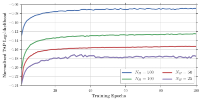
(b) real-MNIST

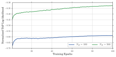
(c) CBCL

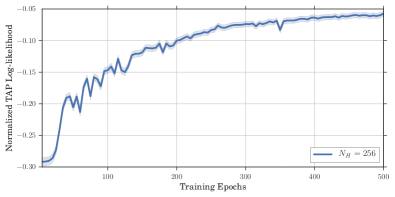
Figure 3: Training performance over 100 epochs for the tested datasets over varying numbers of hidden units, $N_{h}$. Performance is measured in terms of the normalized (per-unit) TAP log-likelihood estimate computed for 10,000 training data samples. The TAP free energy is estimated using the unique TAP solutions thermalized from initial conditions drawn from the data samples, as in (37)–(38). Thermalization is determined by the convergence of the magnetizations up to a difference of $10^{-8}$ in MSE between iterations. Solid lines indicate the average normalized TAP log-likelihood over the tested training samples and shaded regions indicate standard error.

VII.2 Learning Dynamics

We now investigate the behavior of the GRBM over the course of the learning procedure, looking at a few metrics of interest: the TAP-approximated log-likelihood of the training dataset, the TAP free energy, and the number of discovered TAP solutions. We note that each of these metrics is unique to the TAP-based model of the GRBM.

(a) binary-MNIST

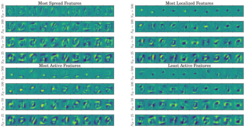
(b) real-MNIST

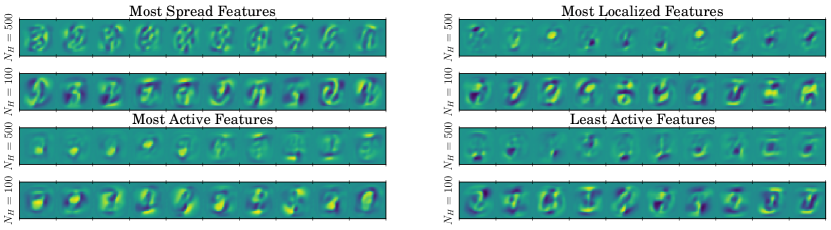
(c) CBCL

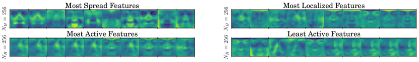
Figure 4: Subsets of the final receptive fields, i.e. the columns of $W$, obtained by TAP training of GRBM models with varying numbers of hidden units, $N_{h}$. For the receptive fields, dark blue and yellow are mapped to $-1$ and $+1$, respectively, and green indicates a value of $0$. Receptive fields are ranked according to two criteria. First, spread, and conversely localization, as measured by the $\ell_{p}$-norm of the receptive field, for $p=0.1$. Second, by activation level, as measured by the mean activation of each receptive field’s corresponding hidden unit averaged across the training dataset.

While it was empirically shown in Gabrié et al. (2015) that CD does indeed increase the TAP log-likelihood in the case of binary RBMs, the specific construction of CD is entirely independent from the TAP model of the GRBM. Thus, it is hard to say that a CD or TAP-trained GRBM is “better” in a general case. At present, we present comparisons between TAP GRBMs of varying complexity trained under fixed hyper-parameters settings, as indicated in Table 1.

In Fig. 3 we see a comparison of the TAP log-likelihood as a function of training epochs for binary-MNIST for binary RBMs consisting of differing numbers of hidden units. As the gradient-ascent on the log-likelihood is performed batch-by-batch over the training data, we define one epoch to be a single pass over the training data: every example has been presented to the gradient ascent once. The specifics of this particular experiment are given in the caption. We note that for equal comparison across varying model complexity, this log-likelihood is normalized over the number of visible and hidden units present in the model. In this way, we observe a “per-unit” TAP log-likelihood, which gives us a measure of the concentration of representational power encapsulated in each unit of the model. Increasing values of the normalized TAP log-likelihood indicate that the evaluated training samples are becoming more likely given the state of the GRBM model parameters.

It can be observed that at each level of complexity, the TAP log-likelihood of the data rapidly increases as the values of $W$ quickly adjust from random initializations to receptive fields correlated with the training data. However, across each of the tested models, by about the $20^{\rm th}$ epoch the rate of increase of the TAP log-likelihood tapers off to a constant rate of improvement.

For reference, we also show a subset of the trained receptive fields, i.e. the rows of $W$, for each of the tested experiments. Since the full set of receptive fields would be too large to display, we attempt to show some representative samples in Fig. 4 by looking at the extreme samples in terms of spatial spread/localization and activity over the training set. We observe that the trained GRBMs, in the case of both binary-MNIST and real-MNIST, are able to learn both the localized and stroke features commonly observed in the literature for binary RBMs trained on the MNIST dataset Hinton (2002); Cho et al. (2013). It is interesting to note that even in the case of real-MNIST, where we are using the novel implementation of truncated Gauss-Bernoulli visible units (see Appendix CC.2), we are able to observe similar learned features as in the case of binary-MNIST. We take this as an empirical indication that the proposed framework of GRBM learning is truly learning correlations present in the dataset as intended. Finally, we see feature localization increase with the number of hidden units.

To date, understanding “what” an RBM learns from the unlabelled data has mostly been a purely subjective exercise in studying the receptive fields, as shown Fig. 4. However, the interpretation of the GRBM as a TAP machine can provide us a novel insight in the nature and dynamics of GRBM learning via the stationary points of the TAP free energy, which we detail in the next section.

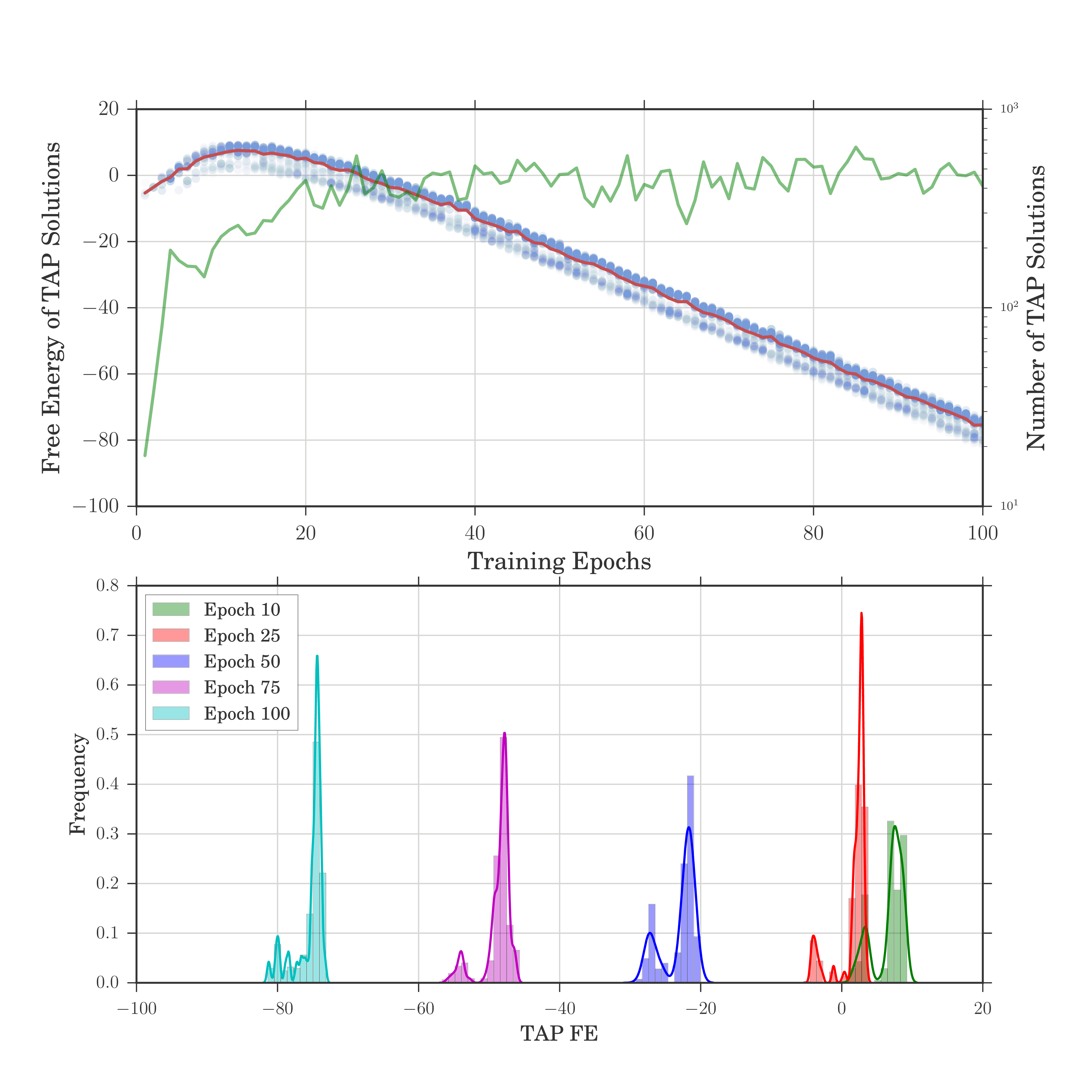
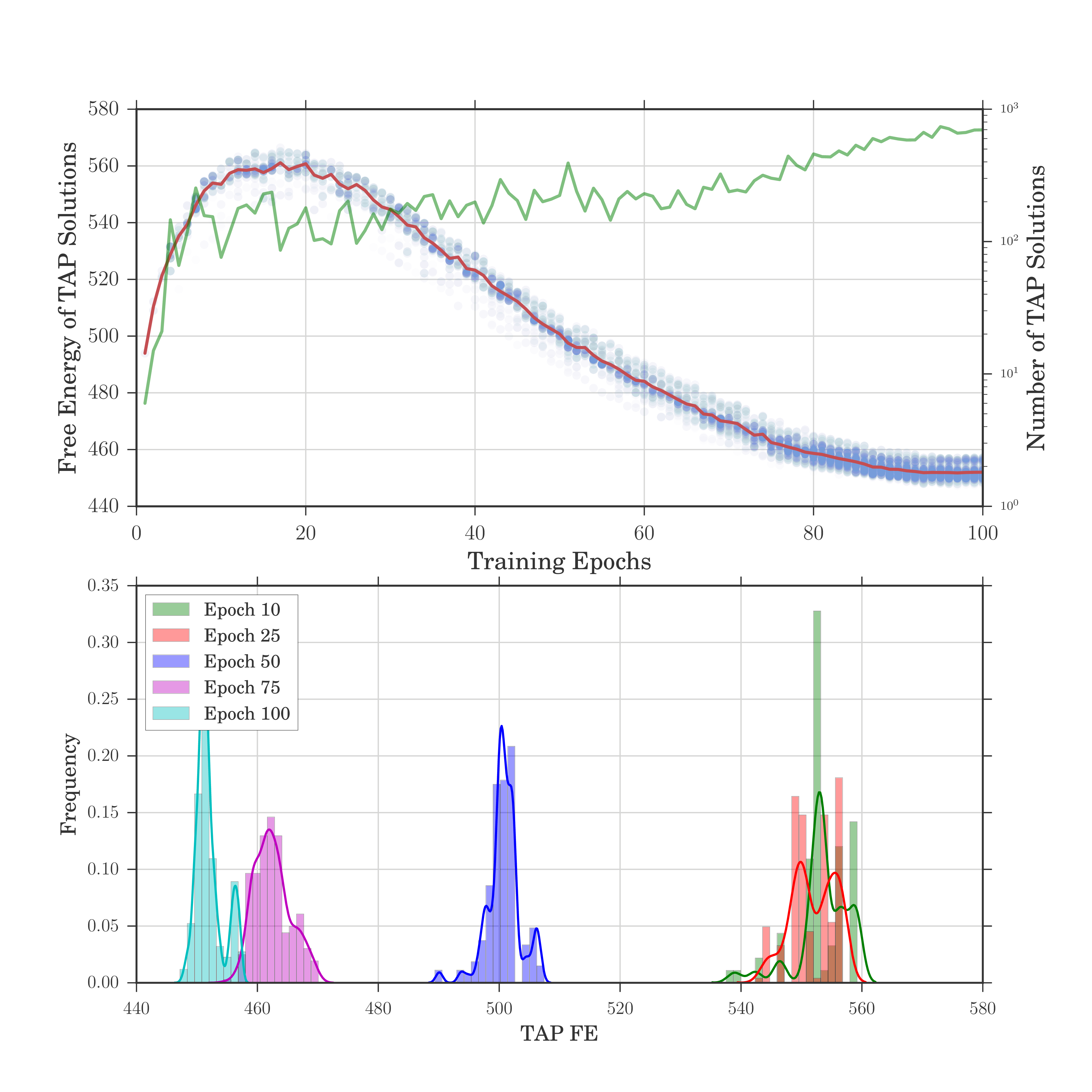
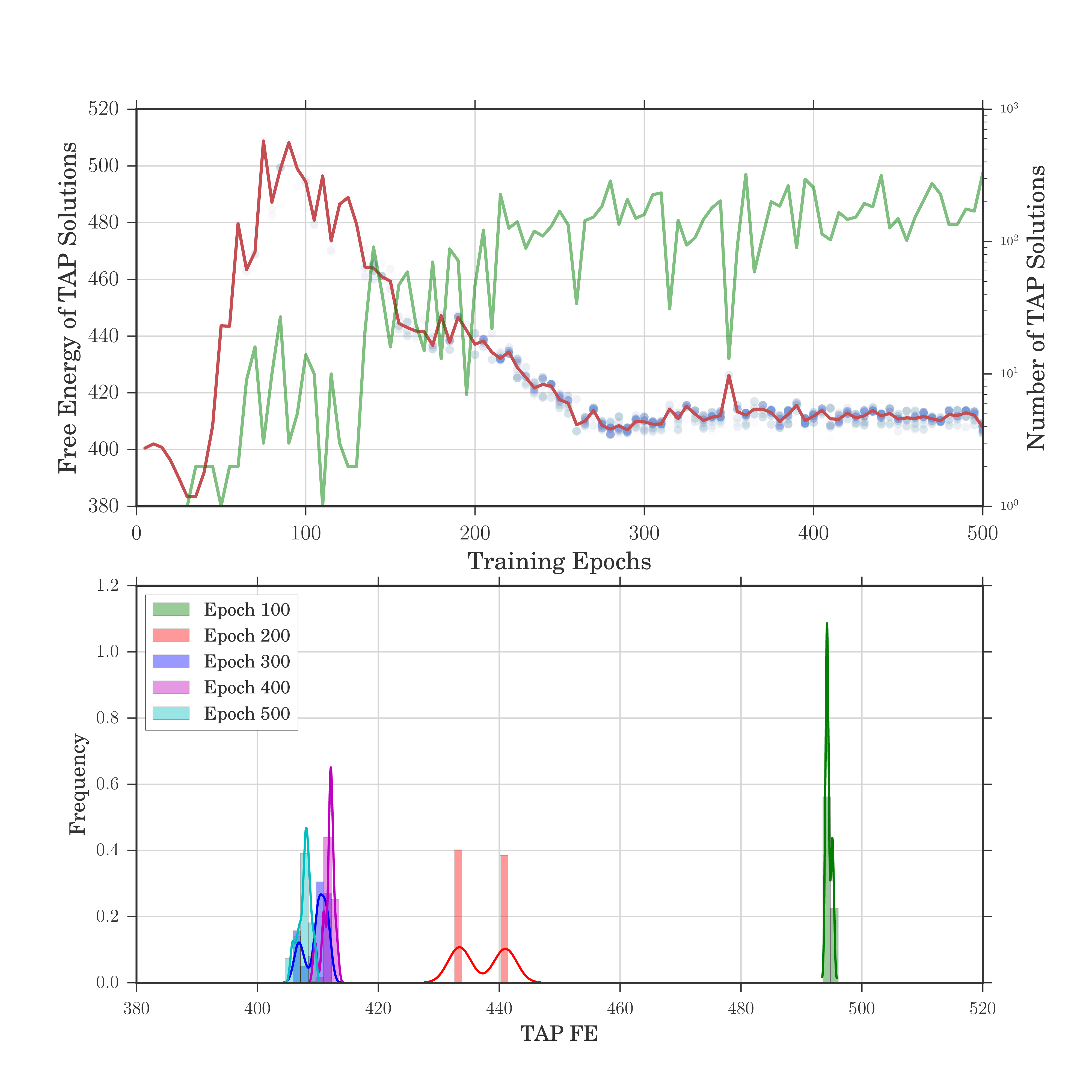
(a) binary-MNIST	(b) real-MNIST	(c) CBCL

Figure 5: Distribution of free energy estimates of TAP solutions as a function of training epochs for the three different datasets. In the case of the two MNIST experiments, the number of hidden units is the same $N_{h}=100$ and $10,000$ samples drawn from the training data are used as initial conditions. For CBCL, $2,400$ training samples are used. Top Row: TAP Free energy for all unique TAP solutions (transparent blue dots), and the Helmholtz free energy estimate via uniform averaging (red line). The number of unique TAP solutions is also given (green line). Bottom Row: Detail of TAP free energy distributions for slices of training. Histograms are given as bars, while kernel density estimates of the TAP free energy distribution are given as curves.

VII.3 Probing the GRBM

Given the deterministic nature of the TAP framework, it is possible to investigate the structure of the modes which a given set of GRBM parameters produces in the free energy landscape. Understanding the nature and concentration of these modes gives us an intuition on the representational power of the GRBM.

To date, observing the modes of a given GRBM model could only be approached via long-chain sampling. Given enough sampling chains from a diverse set of initial conditions, thermalizing these chains produces a set of samples from which one could attempt to derive statistics, such as concentrations of the samples in their high-dimensional space, to attempt to pinpoint the likely modes in the model. However, the number of required chains to resolve these features increases with the dimensionality of the space and the number of potential modes which might exist in the space. Because of this, the numerical evaluation we carry out here would be impractical with sampling techniques.

The r-BP and mean-field models of the RBM allow us to directly obtain the modes of the model by running inference to solve the direct problem. Given a diverse set of initial conditions, such as a given training dataset, running r-BP or TAP provides a deterministic mapping between the initial conditions drawn from the data, as in (37)–(38), and the “nearest” solution of the TAP free energy. If the initial point was drawn from the dataset, then this solution can be interpreted as the RBM’s best-matching internal representation for the data point.

If a large number of structurally diverse data points map to a single solution, then this may be an indicator that the GRBM parameters are not sufficient to model the diverse nature of the data, and perhaps further changes to the model parameters or hyper-parameters are required. Conversely, if the number of solutions explodes, being roughly equivalent to the number of initial data points, then this indicates a potential spin-glass phase, that the specific RBM is over-trained, perhaps memorizing the original data samples during training. Additionally, when in such a phase, the large set TAP solutions may be replete with spurious solutions which convey very little structural information about the dataset. In this case, hyper-parameters of the model may need to be tuned in order to ensure that the model possess a meaningful generalization over the data space.

To observe these effects, we obtain a subset of the TAP solutions by initializing the TAP iteration with initial conditions drawn from the data set, running the iteration until convergence, and then counting the unique TAP solutions. We present some measures on these solutions in Fig. 2. Here, we both count the number of unique TAP solutions, as well as the distribution of the TAP free energy over these solutions, across training epochs. There are a few common features across the tested datasets. First, the early phase of training shows a marked increase of the TAP free energy, which then gradually declines as training continues. Comparing the point of inflection in the TAP free energy against the normalized TAP log-likelihood shown in Fig. 3 shows that the early phase of GRBM training is dominated by the reinforcement of the empirical moments of the training data, with the GRBM model correlations playing a small role in the the gradient of (14). This makes sense, as the random initialization of $W\sim\mathcal{N}(0,\sigma)$ for $\sigma\approx 10^{-3}$ implies that the hidden units are almost independent of the training data. Thus, the TAP solutions at the early stage of learning are driven by, and correlated with, the local potentials on the hidden and visible variables.

The effect of this influence is that the TAP free energy landscape possesses very few modes in the data space. Fig. 5 shows this very clearly, as the number of TAP solutions starts at $1$ and then steadily increases with training. Because the positive data-term of (14) is dominant, the GRBM parameters do not appear to minimize the TAP free energy, as we would expect. However, as more TAP solutions appear, the data and model terms of the gradient become balanced, and the TAP free energy is minimized. It is at this point of inflection that we see leveling off of the normalized TAP log-likelihood.

Second, we observe free-energy bands in the TAP solutions. This feature is especially pronounced in the case of the binary-MNIST experiment. Here, at all training epochs, there exist two significant modes in the free energy distribution over the TAP solutions. We see this effect more clearly in the training-slice histograms shown in the bottom row of Fig. 5(a). In the case of the real-MNIST experiment, we see that the free energy distributions do not exhibit such tight banding, but they do show the presence of some high- and low-energy solutions which persist across training. The main feature across experiments is the multi-modal structure of the free energy distribution. Finally, we note that for both real-MNIST and binary-MNIST, in the case of $N_{h}=100$, we don’t empirically observe an explosion of TAP solutions, a potential indicator a spin-glass phase, since the proportion of unique TAP solutions to the initial data points remains less than 10%.

In order to investigate whether the modes in the TAP free energy distributions are randomly assigned over configuration space, or exist in separate continuous partitions of the configuration space, we need to look at the proximity of the solutions in the configuration space. Because this space cannot be observed in its ambient dimensionality, we project the configuration space into a two-dimensional embedding in Fig. 6. Here, we utilize the well known Isomap Tenenbaum et al. (2000) algorithm for calculating a two-dimensional manifold which approximately preserves local neighborhoods present in the original space. Using this visualization we observe that as training progresses the assignment of high and low free energy to TAP solutions does not appear random in nature, but seems to be inherent to the structure of the solutions themselves, that is, their location in the configuration space. Additionally, in Fig 6 we can see the progression from few TAP solutions to many, and how they spread across the configuration space. It is interesting to note how the solutions start from a highly correlated state and then proceed to diversify.

We can also observe the TAP solutions with respect to the initializations which produced them, as shown in Fig. 7. In these charts, we use a similar approach as Fig. 6, mapping all high-dimensional data points, as well as TAP magnetizations, into a 2D embedding using Isomap. This allows us to see, in an approximate way, how the TAP solutions distribute themselves over the data space. We also show how the number of TAP solutions grows from few to many over training, and how they maintain a spread distribution over the data space. This demonstrates how the training procedure is altering the parameters of the model so as to place TAP solutions within dense regions of the data space. For the sake of clarity, we have not included lines indicating the attribution of an initial data point to its resultant TAP solution. However, as training progresses, one sees that the TAP solutions act as attractors over the data space, clustering together data points which the TAP machine recognizes as similar.

VII.4 Inference for Denoising

Serving as a prior for inference is one particular use case for the TAP machine interpretation of the GRBM. As a simple demonstration, we turn to the common signal processing task of denoising. Specifically, given a planted signal, one observes a set of noisy observations which are measures of the true signal corrupted by some stochastic process. Denoising tasks are ubiquitous in signal processing, both at an analog level (e.g. additive and shot noise), and at the level of digital communications (e.g. binary symmetric and erasure channels). The goal of this task is to produce the most accurate estimate of the unknown signal. In the analog case, this may be a measure of mean-square-error (MSE) between the estimate and the true signal. In the binary case, this may be a measure of accuracy, counting the number of incorrect estimates, or some other function of the binary confusion matrix, such as the F1-score or Matthews correlation coefficient (MCC).

For a fixed set of observations and channel parameters, if we assume that the original signal was drawn from some unknown and intractable generating distribution, then as we construct more and more accurate tractable approximate priors, the more accurately we can construct an estimate of the original signal.

In other words, the more we know about the structure and content of the unknown signal a priori, the closer our estimate can be. Often, as in the case of wavelet-based image denoising, statistics are gathered on the transform coefficients of particular images classes and heuristic denoising approaches are designed by-hand accordingly Şendur and Selesnick (2002). By-hand derivation of denoising algorithms works well in practice owing to its generality. Specific a priori information about the original signal is not required, beyond its signal class (e.g. natural images, human speech, radar return timings). However, meaningful features must be assumed or investigated by practitioners before successful inference can take place.

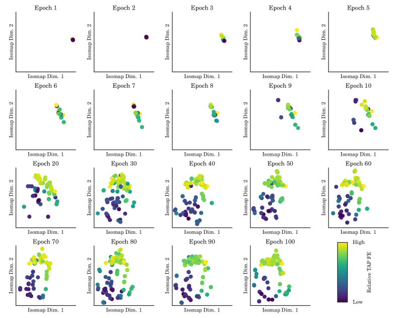
Figure 6: Isomap visualization of TAP solutions for binary-MNIST over training epochs for $N_{h}=100$. All TAP solutions are mapped to the same two-dimensional embedding via an Isomap transform fitted to the TAP solutions of Epoch 100. The embedding is performed on both the hidden and visible inferred expectations, $\mathbf{a}^{\rm v}$ and $\mathbf{a}^{\rm h}$. The color mapping corresponds to the TAP free energy values of each solution, with the range of colors normalized between the minimum and maximum free energies of the solution at each training epoch.

(a) binary-MNIST ($N_{h}=100$)
Epoch 1	Epoch 3	Epoch 25	Epoch 100
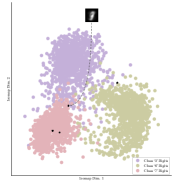
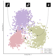
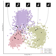
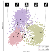
(b) real-MNIST ($N_{h}=500$)
Epoch 1	Epoch 3	Epoch 25	Epoch 100
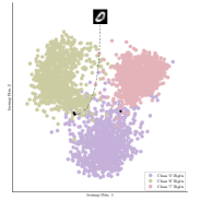
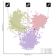
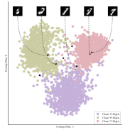
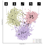
(c) CBCL ($N_{h}=256$)
Epoch 5	Epoch 100	Epoch 200	Epoch 500

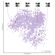
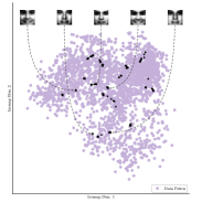
Figure 7: Comparison of initial conditions for TAP equilibration (colored dots) compared to converged TAP solutions (black dots) for the tested datasets at different stages of training. For each dataset, a two-dimensional Isomap embedding is calculated over the initialization data. Subsequently, the magnetizations of the TAP solutions are embedded in the same space. In each case, all initial variances are set to 0, as in Eq. 38. Also, a random selection of TAP solution magnetizations are chosen to provide some context for the representations the RBM is learning. (a) binary-MNIST: Here, the $\sim$3,100 digits corresponding to the classes ‘3’, ‘6’, and ‘7’ are drawn from the first 10,000 training samples of the binarized MNIST dataset as initializations. A reduced set of labels is used for readability. (b) real-MNIST: The same initializations are used as in (a), however, the initializations are not binarized. (c) CBCL: All available training face images are used as initializations.

VII.4.1 Denoising the Binary Symmetric Channel

For binary denoising problems, we assume a binary symmetric channel (BSC) defined in the following manner. Given some binary signal $\mathbf{x}\in\left\{0,1\right\}^{N}$, we observe the signal $\mathbf{y}\in\left\{0,1\right\}^{N}$ as $\mathbf{x}$ with independent bit flips occurring with probability $p$. This gives the following likelihood at each observation,

$$P(\mathbf{y}|\mathbf{x})=(1-p)\prod_{i}\left(\frac{p}{1-p}\right)^{\delta_{x_{i},y_{i}}},$$ (43)

which can be shown to have the equivalent representation as a Boltzmann distribution,

$$P(\mathbf{y}|\mathbf{x})=\frac{1}{Z(\mathbf{y})}e^{\sum_{i}D_{i}x_{i}},$$ (44)

where $D_{i}\triangleq\ln\frac{p}{1-p}(2y_{i}-1)$. For a given prior distribution $P(\mathbf{x})$, the posterior distribution is given by Bayes’ rule,

$$P(\mathbf{x}|\mathbf{y})=\frac{e^{\sum_{i}D_{i}x_{i}}P(\mathbf{x})}{\sum_{\mathbf{x}}e^{\sum_{i}D_{i}x_{i}}P(\mathbf{x})}.$$ (45)

By assuming a factorized $P(\mathbf{x})=\prod_{i}m_{i}^{x_{i}}(1-m_{i})^{1-x_{i}}$, where $m_{i}$ might be per-site empirical averages obtained from available training data, the posterior factorizes and we can construct the Bayes-optimal pointwise estimator (OPE) as the average $\left\langle x_{i}\right\rangle_{P(x_{i}|y_{i})}$ which is just $P(x_{i}=1|y_{i})$ for our binary problem. Thus, the OPE at each site $x_{i}$ is given as

$$P(x_{i}=1|y_{i}) =\frac{1}{1+\left(\frac{1-m_{i}}{m_{i}}\right)\times\left(\frac{1-p}{p}\right)^{2y_{i}-1}},$$

$$={\rm sigm}\left(\ln\frac{m}{1-m}+(2y_{i}-1)\ln\frac{p}{1-p}\right).$$ (46)

For a given dataset, the OPE gives us the best-case performance using only pointwise statistics from the dataset, namely, empirical estimates of the magnetizations $m_{i}$. We can see from Eq. (46) that the OPE either returns the observations, in the case of $p=0$, or the prior magnetizations $m_{i}$, in the case $p=0.5$. In this case of complete information loss, the worst case performance is bounded according to the deviation of the dataset from its mean. We present the performance of the OPE in Fig. 8 for the binary-MNIST dataset. This makes the OPE a valuable baseline comparison and sanity check for the GRBM approximation of $P(\mathbf{x})$. As the GRBM model takes into account both pointwise and pairwise relationships in the data, a properly trained GRBM should provide estimates at least as good as the OPE.

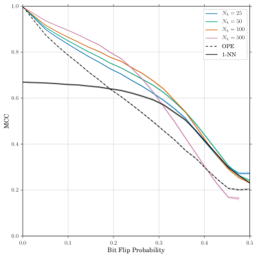
Figure 8: Average denoising performance for reconstruction from bit-flip errors on binary-MNIST over the probability of a bit to be flipped. Denoising via inference on the binary-binary RBM is denoised by the varying numbers of hidden units ($N_{h}=\left\{25,50,100,500\right\}$). Also shown as baseline comparisons are the OPE given the empirical factorized magnetizations at each site (dashed black), and a 1-NN matching from the training set (solid black). All experiments were run over the same 1,000 data samples drawn from the held-out test set and compared using the MCC. Binary estimates are obtained for the OPE and TAP inferred estimates by rounding the resulting magnetizations.

The $k$-Nearest-Neighbor ($k$-NN) algorithm represents a different heuristic approach to the same problem van Ginneken and Mendrik (2006). In this case, the noisy measurements are compared to a set of exemplars: the training dataset. Then, according to some distance metric such as MSE or correlation, one finds the $k$ exemplars with minimal distance to the noisy observations to serve as a basis for recovering the original binary signal. One can use some arbitrary approach for fusing these exemplars together into the final estimate, but the simplest case would be a simple average. In the case that $k\rightarrow\infty$, the performance when using averaging is again bounded by the empirical magnetizations. In the other limit of $k=1$, the estimate is simply the nearest exemplar. It is hard to show the limiting performance of this approach, as it is dependent on the distances, in the chosen metric, between the exemplars and the observations, as well as the interplay between the noise channel and the distance metric.

However, it can be seen directly that this approach is non-optimal, as this approach will not yield the true signal at $p=0$ unless the true signal is itself contained within the training data. We show the performance for $k=1$ in Fig. 8. The advantage of this approach is that it successfully regularizes against noise as $p\rightarrow 0.5$, as the nearest exemplar is always noise-free and at least marginally correlated with the original signal, up to the distance metric. Additionally, we see that it performs better than the OPE in the regime $p>0.2$. This can be explained since we can think of the $k$-NN approach as implicitly, though indirectly, taking into account higher-order correlations in the dataset by naïvely returning data exemplars; all the estimates trivially posses the same arbitrarily complex structure as the unknown signal.

Using the GRBM, we can hope to capture the best points of both approaches. First, we hope to perfectly estimate the original signal in the case $p=0$. Second, we hope to leverage the pairwise correlations present in the dataset, returning estimates which retain the structure of the data even as $p\rightarrow 0.5$. For GRBM denoising of the BSC, we no longer have a factorized posterior. Instead, we have the GRBM likelihood given in Eq. (9) summed over the hidden units. Using the definition of the binary prior given in Appendix C.3,

$$P(\mathbf{x};W,\bm{U})\propto\sum_{\mathbf{h}}e^{\sum_{ij}x_{i}W_{ij}h_{j}+\sum_{i}U_{i}x_{i}+\sum_{j}U_{j}h_{j}}.$$ (47)

Since both the GRBM and the BSC channel likelihood are written as exponential family distributions, $P(\mathbf{y}|\mathbf{x})P(\mathbf{x};W,\bm{U})\propto\sum_{\mathbf{h}}e^{\sum_{ij}x_{i}W_{ij}h_{j}+\sum_{i}(D_{i}+U_{i})x_{i}+\sum_{j}U_{j}h_{j}}$. Finding the averages $\left\langle x_{i}\right\rangle$ for this model simply consists in running the TAP-based inference of Alg. 1 for the modified visible binary prior $\mathcal{B}(x_{i};U_{i}+D_{i})$. One heuristic caveat of this approach is that we must take into account the multi-modal nature of the TAP free energy. Since we must initialize somewhere, and the resulting inference estimate is dependent upon this initialization, we initialize the inference with the OPE result.

We can see that as $p\rightarrow 0$, $D_{i}\rightarrow\pm\infty$ and the highest probability configuration becomes observations. So, in the limit, we are able to obtain the true signal, just as the OPE, especially since we initialize within the well of this potential. This is shown for binary RBMs trained with varying numbers of hidden units in Fig. 8. In every case, for $p=0$, the true signal is recovered. In the case of $N_{h}=\left\{25,50,100\right\}$, we see that the TAP inference on the binary RBM always outperforms the OPE. Additionally, we see that in each of these cases, the performance closely mirrors that of the $1$-NN as $p\rightarrow 0.5$. In the limit $p=0.5$, we see that the result of the TAP inference is, essentially, uncorrelated with the original signal, as in this case, there is no extra potential present to bias the inference, and the resulting estimate is simply an arbitrary solution of the TAP free energy. As this closely mirrors the exemplar selection in $1$-NN, the MCC curves for the two approaches are similar.

In the case of $N_{h}=500$, we can see that an over-training effect occurs. Essentially, at low values of $p$, the TAP inference over the binary RBM is able to more accurately identify the original signal. However, at a certain point, owing to the increased number of solutions in the TAP free energy, there exist many undesirable minima around the noisy solutions, leading to poor denoising estimates. One can observe this subjectively in Fig. 9, where in the case of $N_{h}=500$, the TAP inference results in either nearly zero-modes, or in very localized ones. This would seem to indicate that landscape of the TAP free energy around the initializations is becoming more unstable as the density of solutions increases around it. Additionally, since the TAP free energy landscape was only probed using data points during training, the clustering of solutions around noisy samples remains ambiguous. Augmenting the initializations used when calculating the TAP solutions for the gradient estimate with noisy data samples could help alleviate this problem and regularize the TAP free energy landscape in the space of noisy data samples.

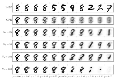
Figure 9: Subjective comparison of denoising estimates for a single digit image for $p=\left[0,0.5\right]$. For the OPE and RBM approaches, the inferred posterior averages $\left\langle x_{i}\right\rangle$ are shown, rather than the final configurations, where white and black represent the values $0$ and $1$, respectively. At each tested value of $p$, the same noise realization is used for each method. As $p$ increases, for $N_{h}=\left\{25,50,100\right\}$, the TAP inference for the RBM provides estimates which still possess digit structure. In the case $N_{h}=500,$ the TAP inference gets caught in spurious and undesirable minima as $p$ increases.

VIII Discussion

In this paper, we have proposed a novel interpretation of the RBM within a fully tractable and deterministic framework of learning and inference via TAP approximation. This deterministic construction allows novel tools for scoring unsupervised models, investigation of the memory of trained models, as well as allowing their efficient use as structured joint priors for inverse problems. While deterministic methods based on NMF for RBM training were shown to be inferior to CD-k in Welling and Hinton (2002), the level of approximation accuracy afforded by TAP finally makes the deterministic approach to RBMs effective, as shown in the case of binary RBMs in Gabrié et al. (2015).

Additionally, our construction is generalized over the distribution of both the hidden an visible units. This is unique to our work, as other works propose unique training methods and models when changing the distribution of the visible units. For example, this can be seen in the modified Hamiltonians used for real-valued data Melchior et al. (2017); Cho et al. (2011). This construction allows us to consider binary, real-valued, and sparse real-valued datasets within the same framework. Additionally, one can also consider other architectures by changing the distributions imposed on the hidden unit. Here, we present experiments using only binary hidden units, but one could also use our proposed framework for Gaussian-distributed hidden units, thus mimicking a Hopfield network Hopfield (1982). Or, also, sparse Gauss-Bernoulli distributed hidden units could mimic the same functionality as that proposed by the spike-and-slab RBM Courville et al. (2011). We have left these investigations to further works on this topic.

Our proposed framework also offers a possibility to explore the statistical mechanics of these latent variable models at the level of TAP approximation. Specifically, for a given statistical model of the weights $W$, both the cavity method and replica can begin to make predictions about these unsupervised models. Analytical understanding of the complexity of the free energy landscape, and its transitions as a function of model hyper-parameters, can allow for a richer understanding of statistically optimal network construction for learning tasks. In the case of random networks, there has already been some progress in this area, as shown in Tubiana and Monasson (2016) and Barra et al. (2016). However, similar comprehensive studies conducted on learning in a realistic setting are still yet to be realized. Finally, as our framework can be applied to deep Boltzmann machines with minimal alteration, it can also potentially lead to a richer understanding of deep networks and the role of hierarchy in regularizing the learning problem in high dimensionality.

Appendix A Belief Propagation for Pairwise Models

In order to estimate the derivatives of $\mathbb{F}$, we must first construct a BP algorithm on the factor graph representation given in Fig. 1. We note that this graph, in terms of the variables $\mathbf{x}$, does not make an explicit distinction between the latent and visible variables. We instead treat this graph in full generality so as to clarify the derivation and notation. This graph corresponds to the following joint distribution over $\mathbf{x}$,

$$P(\mathbf{x};W,\bm{\theta})\propto e^{\sum_{(i,j)}\phi(x_{i},x_{j};W_{ij})+\sum_{i}\phi(x_{i};\theta_{i})},$$ (48)

where $\sum_{(i,j)}$ is a sum over the edges in the graph. In the case of a Boltzmann machine, any two variables are connected via pairwise factors,

$$\phi(x_{i},x_{j};W_{ij})=e^{W_{ij}x_{i}x_{j}},$$ (49)

and all variables are also influenced by univariate factors written trivially as $\phi(x_{i};\theta_{i})=P_{i}(x_{i};\theta_{i})$.

A message-passing can be constructed on this factor graph by writing messages from variables to factors and also from factors to variables. Since all factors are at most degree 2, we can write the messages for this system as variable to variable messages Mézard and Montanari (2009),

$$\nu_{i\to j}^{(t+1)}(x_{i})=\frac{\phi(x_{i};\theta_{i})}{Z_{i\rightarrow j}}\prod_{l\in\partial_{i}/j}\int{\rm d}x_{l}~{}~{}\phi(x_{i},x_{l};W_{il})~{}\nu^{(t)}_{l\rightarrow i}(x_{l}).$$ (50)

Here, the notation $i\rightarrow j$ represents a message from variable index $i$ to variable index $j$, and $\partial_{i}/j$ refers to all neighbors of variable index $i$ except variable index $j$. We denote neighboring variables as those which share a pairwise factor. Finally, the super-scripts on the messages refer to the time-index of the BP iteration, which implies the successive application of (50) until convergence on the set of messages $\underset{\bar{}}{\nu}=\left\{\nu_{i\rightarrow j}(x_{i}):(i,j)\in E\right\}$, where $E$ is the set of all pairs of neighboring variables. We also note the inclusion of the message normalization term $Z_{i\rightarrow j}$ which ensures that all messages are valid PDFs. Additionally, it is possible to write the marginal beliefs at each variable by collecting the messages from all their neighbors,

$$\nu^{(t)}_{\rightarrow i}(x_{i})=\frac{\phi(x_{i};\theta_{i})}{Z_{\rightarrow i}}\prod_{j\in\partial_{i}}\int{\rm d}x_{j}~{}~{}\phi(x_{i},x_{j};W_{ij})~{}\nu^{(t)}_{j\rightarrow i}(x_{j}).$$ (51)

Subsequently, the Bethe free energy can be written for a converged set of messages, $\underset{\bar{}}{\nu}^{*}$, according to Mézard and Montanari (2009) as

$$\mathbb{F}_{\rm B}[\underset{\bar{}}{\nu}^{*}]=\sum_{i}\mathbb{F}_{i}[\underset{\bar{}}{\nu}^{*}]-\sum_{(i,j)\in E}\mathbb{F}_{(i,j)}[\underset{\bar{}}{\nu}^{*}]=\sum_{i}\ln Z_{\rightarrow i}^{*}-\sum_{(i,j)}\ln\left[\int{\rm d}x_{i}~{}{\rm d}x_{j}~{}~{}\nu_{i\rightarrow j}^{*}(x_{i})~{}\phi(x_{i},x_{j};W_{ij})~{}\nu_{j\rightarrow i}^{*}(x_{j})\right],$$ (52)

where $Z_{\rightarrow i}^{*}$ refers to the normalization of the set of the marginal belief at site $i$ derived from $\underset{\bar{}}{\nu}^{*}$.

Unfortunately, the message-passing of (50) cannot be written as a computable algorithm due to the continuous nature of the PDFs. Instead, we must find some manner by which to parameterize the messages. In the case of binary variables, as in Gabrié et al. (2015), each message PDF can be exactly parameterized by its expectation. However, for this general case formulation, we cannot make the same assumption. Instead, we turn to relaxed BP (r-BP) Rangan (2010), described in the next section, which assumes a two-moment parameterization of the messages.

Appendix B r-BP for Pairwise Models

We will now consider one possible parametric approximation of the message set via r-BP Rangan (2010). This approach has also gone by a number of different names in parallel re-discoveries of the approach, e.g. moment matching Opper and Winther (2005) and non-parametric BP Sudderth et al. (2010). In essence, we will be assuming that all messages $\underset{\bar{}}{\nu}$ can be well-approximated by their mean and variance, a Gaussian assumption. This approximation arises from a second-order expansion assuming small weights $W_{ij}$. By making this assumption, we will ultimately be able to close an approximation of the messages on their two first moments, $a_{i\rightarrow j}\triangleq\left\langle x_{i}\right\rangle_{\nu_{i\rightarrow j}}$ and $c_{i\rightarrow j}\triangleq\left\langle x_{i}^{2}\right\rangle_{\nu_{i\rightarrow j}}-\left\langle x_{i}\right\rangle^{2}_{\nu_{i\rightarrow j}}$.

B.1 Derivation via Small Weight Expansion

Considering the marginalization taking place in (50), we will perform a second order expansion assuming that $W_{il}\rightarrow 0$. We start by taking the Taylor series of the incoming message marginal for negligible weights,

$$\int{\rm d}x_{l}~{}~{}e^{W_{il}x_{i}x_{l}}\cdot\nu^{(t)}_{l\rightarrow i}(x_{l})=$$

$$\quad 1+W_{il}\int{\rm d}x_{l}~{}~{}\frac{\partial}{\partial W_{il}}\left[e^{W_{il}x_{i}x_{l}}\right]_{W_{il}=0}\nu^{(t)}_{l\rightarrow i}(x_{l})$$

$$\quad+\frac{1}{2}W_{il}^{2}\int{\rm d}x_{l}~{}~{}\frac{\partial}{\partial W_{il}^{2}}\left[e^{W_{il}x_{i}x_{l}}\right]_{W_{il}=0}\nu^{(t)}_{l\rightarrow i}(x_{l})$$

$$\quad+O(W_{il}^{3}).$$ (53)

Now, we approximate the series by dropping the terms less than $O(W_{il}^{3})$. This approximation can be justified in the event that all weight values satisfy $|W_{il}|<1$. Identifying the integrals from the expansion as moments, we see the following approximation

$$\approx 1+x_{i}W_{il}a_{l\rightarrow i}^{(t)}+\frac{1}{2}x_{i}^{2}W_{il}^{2}\left\langle x_{l}^{2}\right\rangle_{\nu_{l\rightarrow i}^{(t)}}.$$ (54)

However, we would like to write this approximation in terms of the central second moment. Through a second approximation that neglects $O(W_{il}^{3})$ terms we arrive at our desired parameterization of the incoming message marginalization in terms of the message’s two first central moments,

$$=\exp\left\{\log\left[1+x_{i}W_{il}a_{l\rightarrow i}^{(t)}+\frac{1}{2}x_{i}^{2}W_{ij}^{2}\left\langle x_{l}^{2}\right\rangle_{\nu_{l\rightarrow i}^{(t)}}\right]\right\},$$

$$\approx e^{x_{i}W_{il}a_{l\rightarrow i}^{(t)}+\frac{1}{2}x_{i}^{2}W_{il}^{2}c_{l\rightarrow i}^{(t)}+O(W_{il}^{3})},$$

$$\approx e^{x_{i}W_{il}a_{l\rightarrow i}^{(t)}+\frac{1}{2}x_{i}^{2}W_{il}^{2}c_{l\rightarrow i}^{(t)}}.$$ (55)

We now substitute this approximation back into (50) to get

$$\nu_{i\to j}^{(t+1)}(x_{i})\approx\widetilde{\nu}_{i\to j}^{(t+1)}(x_{i})=\frac{\phi(x_{i};\theta_{i})}{Z_{i\rightarrow j}}e^{x_{i}B_{i\rightarrow j}^{(t)}-\frac{1}{2}x_{i}^{2}A_{i\rightarrow j}^{(t)}},$$ (56)

where

$$B_{i\rightarrow j}^{(t)} \triangleq\sum_{l\in\partial_{i}/j}W_{il}a_{l\rightarrow i}^{(t)},$$ (57)

$$A_{i\rightarrow j}^{(t)} \triangleq-\sum_{l\in\partial_{i}/j}W_{il}^{2}c_{l\rightarrow i}^{(t)}.$$ (58)

From here, we can see that we have now a set of closed equations due to the dependence of $\mathbf{A}^{(t)}$ and $\mathbf{B}^{(t)}$ on the moments $\mathbf{a}^{(t)}$ and $\mathbf{c}^{(t)}$, and vice versa. The values of these moments can be written as a function of $\mathbf{A}^{(t)}$ and $\mathbf{B}^{(t)}$ which is dependent upon the form of the local potentials $\phi(x_{i};\theta_{i})$, i.e. the prior distribution we assign to the variables themselves,

$$a^{(t)}_{i\rightarrow j} =f_{\rm a}\left(B^{(t-1)}_{i\rightarrow j},A^{(t-1)}_{i\rightarrow j};\theta_{i}\right),$$ (59)

$$c^{(t)}_{i\rightarrow j} =f_{\rm c}\left(B^{(t-1)}_{i\rightarrow j},A^{(t-1)}_{i\rightarrow j};\theta_{i}\right),$$ (60)

where

$$f_{\rm a}\left(B,A;\theta\right)\triangleq \int{\rm d}x~{}~{}x~{}\frac{\phi(x;\theta)}{Z}~{}e^{xB-\frac{1}{2}x^{2}A},$$ (61)

$$f_{\rm c}\left(B,A;\theta\right)\triangleq -f_{\rm a}\left(B,A;\theta\right)^{2}+$$

$$\int{\rm d}x~{}~{}x^{2}~{}\frac{\phi(x;\theta)}{Z}~{}e^{xB-\frac{1}{2}x^{2}A},$$ (62)

and $Z$ is simply the normalization $\int{\rm d}x~{}~{}\phi(x;\theta)~{}e^{xB-\frac{1}{2}x^{2}A}$. The inferred marginal distributions at each site can be calculated via the same functions, but instead using all of the incoming messages, i.e. $a^{(t)}_{i}=f_{\rm a}\left(B^{(t)}_{\rightarrow i},A^{(t)}_{\rightarrow i};\theta_{i}\right)$ and $c^{(t)}_{i}=f_{\rm c}\left(B^{(t)}_{\rightarrow i},A^{(t)}_{\rightarrow i};\theta_{i}\right)$. In Appendix C.1 we give the closed-forms of these moment calculations for a few different choices of $\phi(x;\theta)$.

If one wants to obtain an estimate of the free energy for a given set of parameters $\bm{\theta}$, it is possible to iterate between (58), (57) and (59), (60) until, ideally, convergence. It is important to note, however, due to both the potentially loopy nature of the network as well as small-weight expansion, that the BP iteration is not guaranteed to converge Welling and Teh (2003); Mézard and Montanari (2009). Additionally, while we retain the time-indices in our derivation, it is not clear whether one should attempt to iterate these message in fully sequential or parallel fashion, or if some clustering and partitioning of the variables should be applied to determine the update order dynamically.

B.2 r-BP Approximate Bethe Free Energy

Additionally, we can write the specific form of the Bethe free energy under the r-BP two-moment parameterization of the messages. In this case, we can simply apply the small weight expansion of (55) to the Bethe free energy for pairwise models given in (52),

$$\widetilde{\mathbb{F}}_{\rm B}[\widetilde{\underset{\bar{}}{\nu}}^{*}] =\sum_{i}\ln\widetilde{Z}_{\rightarrow i}^{*}$$

$$\quad-\sum_{(i,j)}\ln\left[\int{\rm d}x_{i}~{}\widetilde{\nu}_{i\rightarrow j}^{*}(x_{i})~{}e^{x_{i}W_{ij}a_{j\rightarrow i}^{*}+\frac{1}{2}x_{i}^{2}W_{ij}^{2}c_{j\rightarrow i}^{*}}\right].$$ (63)

Subsequently, using the final message definition given in (56), we can see that

$$\widetilde{\mathbb{F}}_{\rm B}[\widetilde{\underset{\bar{}}{\nu}}^{*}] =\sum_{i}\ln\widetilde{Z}_{\rightarrow i}^{*}-\sum_{(i,j)}\left\{\ln\widetilde{Z}_{\rightarrow i}^{*}-\ln\widetilde{Z}_{i\rightarrow j}^{*}\right\},$$ (64)

which, correcting for double counting, can also be written as

$$\widetilde{\mathbb{F}}_{\rm B}[\widetilde{\underset{\bar{}}{\nu}}^{*}]=\sum_{i}(1-\frac{1}{2}d_{i})\ln\widetilde{Z}_{\rightarrow i}^{*}+\frac{1}{2}\sum_{i,j}\ln\widetilde{Z}_{i\rightarrow j}^{*},$$ (65)

where $d_{i}$ is the degree at site $i$, $|\partial_{i}|$.

B.3 Enforcing Bounded Messages

While we write the r-BP messages (56) as though they are Gaussian distributions, this is a slight, since $A_{i\rightarrow j}^{(t)}\leq 0$ as $W_{il}^{2}c_{l\rightarrow i}^{(t)}\geq 0~{}~{}\forall i,l$. The implication of the expansion is that, in general, the messages are in fact unbounded. This unboundedness is a direct result of the form of the conventional RBM pairwise factor, $e^{x_{i}W_{ij}x_{j}}$.

There are a few avenues available to us to address these unbounded messages and produce a meaningful message-passing for generalized RBMs. Let us consider the cases for which the messages are unbounded given a specific variable distribution. Assume that site $x_{i}$ is assigned a Gaussian prior, $\phi(x_{i};\theta_{i}=\left\{V_{i},U_{i}\right\})\propto e^{x_{i}U_{i}-\frac{1}{2}x_{i}^{2}V_{i}}$. In this case the r-BP message reads

$$\widetilde{\nu}_{i\to j}^{(t+1)}(x_{i}) =\frac{1}{\widetilde{Z}_{i\rightarrow j}}e^{x_{i}(U_{i}+B_{i\rightarrow j}^{(t)})-\frac{1}{2}x_{i}^{2}(V_{i}+A_{i\rightarrow j}^{(t)})}.$$ (66)

In this case, the message is unbounded in the event that weighted sum of all incoming neighbor variances at $i$ exceeds the inverse variance of Gaussian prior on $x_{i}$,

$$V_{i}+A_{i\rightarrow j}^{(t)} <0,$$ (67)

$$V_{i} <\sum_{l\in\partial_{i}/j}W_{il}^{2}c_{l\rightarrow i}^{(t)},$$ (68)

$$\sigma_{i}^{2} >\left[\sum_{l\in\partial_{i}/j}W_{il}^{2}c_{l\rightarrow i}^{(t)}\right]^{-1},$$ (69)

where $\sigma_{i}^{2}$ is the variance of the Gaussian prior. Said another way, this condition is telling us that when the message-passing starts to tell us that if the variance at $x_{i}$ is smaller than that of its prior, the messages become unbounded and fail to be meaningful probability distributions, and our expansion fails. The implication is that the r-BP message passing should be utilized in contexts where there exists some, preferably strong, evidence at each site, or the weights in $W$ should be sufficiently small. The stronger this local potential, or the smaller the weights, the more favorable the model is to the r-BP inference. This observation mirrors those made in Welling and Teh (2003), however, here the authors make the observation that in this setting, BP based on small-weight expansion for binary variables fails to converge. In our case, without taking some form of regularization, the inference fails entirely. Thus, large magnitude couplings $W_{il}$ must be backed with a high degree of evidence at site $i$ and $l$. This property could be utilized for the inverse learning problem, where one must learn the couplings $W$ given a dataset, in order to constrain the learning to parameters which are amenable to the r-BP inference.

One direct manner to create probability distributions from otherwise unbounded continuous functions is via truncation. Specifically, we enforce a non-infinite normalization factor by restricting the support of the distribution to some subset of $\mathbb{R}$. In this case, just slightly violating the bounded condition above will induce a uniform message distribution over the distribution support, while a strong violation will cause the distribution to concentrate on the boundaries of the support. Another approach might simply be to fix a hard boundary constraint on $A_{i\to j}$, thus never permitting unbounded messages to occur.

Appendix C Calculations for Specific Variable Distributions

C.1 Truncated Gaussian Units

In general, the truncated Gaussian is defined in the following manner,

$$\mathcal{TG}(x;\mu,\sigma^{2},[\alpha,\omega])=\frac{1}{\sqrt{2\pi\sigma^{2}}}\cdot\frac{1}{\Phi\!\!\left[\frac{\omega-\mu}{\sigma}\right]-\Phi\!\!\left[\frac{\alpha-\mu}{\sigma}\right]}\cdot e^{-\frac{(x-\mu)^{2}}{2\sigma^{2}}},$$ (70)

where $\mu$ and $\sigma^{2}$ are the mean and variance of the original Gaussian prior to truncation and the range $[\alpha,\omega]$ defines the lower and upper bounds of the truncation, $-\infty\leq\alpha<\omega\leq\infty$, and $\Phi\left[\cdot\right]$ is the CDF for the Normal distribution. To make things easier for us later, we will define the prior in a little bit of a different manner by making the following definitions,

$$V\triangleq\frac{1}{\sigma^{2}},\quad\quad U\triangleq\frac{\mu}{\sigma^{2}},$$ (71)

and writing the distribution for the parameters $\theta=\left\{U,V,[\alpha,\omega]\right\}$ as

$$\mathcal{TG}_{+}(x;\theta)=\frac{\frac{2}{e^{\frac{U^{2}}{2V}}}\sqrt{\frac{V}{2\pi}}e^{-\frac{1}{2}Vx^{2}+Ux}}{{\rm Erf}\!\left[\sqrt{\frac{V}{2}}(\omega-\frac{U}{V})\right]-{\rm Erf}\!\left[\sqrt{\frac{V}{2}}(\alpha-\frac{U}{V})\right]},$$ (72)

where ${\rm Erf}\!\left[\cdot\right]$ is the error function and the last step follows from the identity $\Phi\!\!\left[x\right]=\frac{1}{2}+\frac{1}{2}{\rm Erf}\!\left[\frac{x}{\sqrt{2}}\right]$. Here, the subscript $+$ is used to indicate $V>0$.

In the case that $V<0$, we will write $\mathcal{TG}$ in terms of the imaginary error function, ${\rm Erfi}\!\left[x\right]\triangleq-i{\rm Erf}\!\left[ix\right]$, and noting that for $V<0$, $V=-1\cdot|V|$,

$$\mathcal{TG}_{-}(x;\theta)=\frac{\frac{2}{e^{\frac{U^{2}}{2V}}}\sqrt{\frac{|V|}{2\pi}}e^{-\frac{1}{2}Vx^{2}+Ux}}{{\rm Erfi}\!\left[\sqrt{\frac{|V|}{2}}(\omega-\frac{U}{V})\right]-{\rm Erfi}\!\left[\sqrt{\frac{|V|}{2}}(\alpha-\frac{U}{V})\right]}.$$ (73)

We use this negative variance version of the truncated Gaussian to handle the special case of $A+V<0$ first detailed in Sec. B.3.

We now detail the computation of the partition and first two moments of the Gaussian-product distribution of $\mathcal{TG}$,

$Q(x;\theta,A,B)=\frac{1}{Z}\mathcal{TG}(x;\theta)e^{-\frac{1}{2}Ax^{2}+Bx}$. The calculation of the moments as a function of $A$ and $B$ will provide the definitions of $f_{\rm a}$ and $f_{\rm c}$, while the calculation of the normalization $Z$ will provide terms necessary for both the computation of the TAP free energy as well as the gradients necessary for learning $\theta$ during RBM training.

First, we will calculate the normalization of $Q(x;\theta,A,B)$ in terms of all free parameters. To do this, consider the truncated normalization of the following product of Gaussians,

$$Z_{Q}=\frac{1}{Z_{\mathcal{TG}}}\int_{\alpha}^{\omega}{\rm d}x~{}~{}e^{-\frac{1}{2}(A+V)x^{2}+(B+U)x},$$ (74)

where $Z_{\mathcal{TG}}$ is defined such that $\mathcal{TG}(x;\theta)=\frac{1}{Z_{\mathcal{TG}}}e^{-\frac{1}{2}Vx^{2}+Ux}$. We will need to make note of the special case of $A+V<0$, thus,

$$Z_{Q}=\frac{1}{Z_{\mathcal{TG}}}\sqrt{\frac{\pi}{2|A+V|}}e^{\frac{(B+U)^{2}}{2(A+V)}}\times\left\{\begin{array}[]{lr}d_{+},&A+V>0\\ d_{-},&A+V<0\end{array}\right.,$$ (75)

where $d_{+}\triangleq{\rm Erf}\!\left[h_{\omega}\right]-{\rm Erf}\!\left[h_{\alpha}\right]$, $d_{-}\triangleq{\rm Erfi}\!\left[h_{\omega}\right]-{\rm Erfi}\!\left[h_{\alpha}\right]$, and $h_{x}\triangleq\sqrt{\frac{|A+V|}{2}}\left(x-\frac{B+U}{A+V}\right)$.

Since $Q(x;\theta,A,B)$ is simply a truncated Gaussian with updated parameters, the first moment is given according to the well known truncated Gaussian expectation. While this expectation is usually written in terms of a mean and variance of the un-truncated Gaussian distribution, and for the case of positive mean, we will instead write the expectation in terms of the exponential polynomial coefficients and note the special case $A+V<0$,

$$f_{\rm a}(B,A;\theta) =\frac{B+U}{A+V}+\sqrt{\frac{2}{\pi|A+V|}}$$

$$\quad\times\left\{\begin{array}[]{lr}\frac{e^{-h_{\alpha}^{2}}-e^{-h_{\omega}^{2}}}{d_{+}},&A+V>0\\ \frac{e^{h_{\alpha}^{2}}-e^{h_{\omega}^{2}}}{d_{-}},&A+V<0\end{array}\right..$$ (78)

Next, we will write the variance of $Q(x;\theta,A,B)$ as a function of $A$ and $B$. As earlier, since $Q$ has the specific form of a truncated Gaussian distribution we can utilize the well-known variance formula for such a distribution. As in the case of $f_{\rm a}$, we modify this function for the special case of $A+V<0$. Specifically,

$$f_{\rm c}(B,A;\theta)=\frac{1}{A+V}-\left(f_{\rm a}(B,A;\theta)-\frac{B+U}{A+V}\right)^{2}$$

$$\quad\quad+\frac{2}{\sqrt{\pi}(A+V)}\times\left\{\begin{array}[]{lr}\frac{h_{\alpha}e^{-h_{\alpha}^{2}}-h_{\omega}e^{-h_{\omega}^{2}}}{d_{+}},&A+V>0\\ \frac{h_{\alpha}e^{h_{\alpha}^{2}}-h_{\omega}e^{h_{\omega}^{2}}}{d_{-}},&A+V<0\end{array}\right..$$ (81)

C.1.1 Gradients of the Log-likelihood

To determine the gradients of the log-likelihood w.r.t. the model parameters, it is necessary to calculate the gradients of both $\ln\mathcal{TG}_{+}(x;\theta)$ and $\ln Z_{Q}$ in terms of the distribution parameters $U$ and $V$. We assume that the boundary terms $\alpha$ and $\omega$ remain fixed. Since both of these distributions are truncated Gaussians, we can treat them both in terms of the derivatives of the log normalization of a general-case truncated Gaussian,

$$\ln Z_{\mathcal{TG}}=-\frac{U^{2}}{2V}+\frac{1}{2}\ln|V|-\ln d_{+/-}.$$ (82)

For Boltzmann measures of the given quadratic form, we know that $\frac{\partial}{\partial U}{\ln Z_{\mathcal{TG}}}=\left\langle x\right\rangle_{\mathcal{TG}}$ and $\frac{\partial}{\partial V}{\ln Z_{\mathcal{TG}}}=-\frac{1}{2}\left\langle x^{2}\right\rangle_{\mathcal{TG}}$. From these relations, we can write the necessary derivatives. For the case of $\ln\mathcal{TG}_{+}(x;\theta)$ we have

$$\frac{\partial}{\partial U}{\ln\mathcal{TG}_{+}(x;\theta)} =x-\frac{\partial}{\partial U}\ln Z_{\mathcal{TG}}=x-\left\langle x\right\rangle_{\mathcal{TG}},$$ (83)

and

$$\frac{\partial}{\partial V}{\ln\mathcal{TG}_{+}(x;\theta)} =-\frac{1}{2}x^{2}-\frac{\partial}{\partial V}\ln Z_{\mathcal{TG}},$$

$$=-\frac{1}{2}\left(x^{2}-\left\langle x^{2}\right\rangle_{\mathcal{TG}}\right),$$ (84)

which we can see as just the difference between the data and the moments of the truncated Gaussian distribution.

Next, the derivatives of $Z_{Q}$, for fixed $A$ and $B$, can be written in terms of $f_{\rm a}$ and $f_{\rm c}$, the moments of $Q$,

$$\frac{\partial}{\partial U}\ln Z_{Q} =f_{a}(B,A;\theta)-\left\langle x\right\rangle_{\mathcal{TG}},$$ (85)

$$\frac{\partial}{\partial V}\ln Z_{Q} =-\frac{1}{2}\left(f_{c}(B,A;\theta)+f_{a}(B,A;\theta)^{2}-\left\langle x^{2}\right\rangle_{\mathcal{TG}}\right).$$ (86)

Finally, we are ready to write the gradients of the log-likelihood to be used for both hidden and visible updates with the truncated Gaussian distribution. For a given set of mini-batch data indexed by $m\in\left\{1,\dots,M\right\}$, and a number of TAP solutions indexed by $p\in\left\{1,\dots,P\right\}$, the gradients of a visible variable are given by

$$\Delta U_{i} =\frac{1}{M}\sum_{m}\left(x_{i}^{(m)}-\left\langle x_{i}\right\rangle_{\mathcal{TG}}\right)$$

$$\quad-\frac{1}{P}\sum_{p}\left(a_{i}^{(p)}-\left\langle x_{i}\right\rangle_{\mathcal{TG}}\right),$$

$$=\left\langle x_{i}\right\rangle_{M}-\left\langle a_{i}\right\rangle_{P},$$ (87)

and

$$\Delta V_{i} =-\frac{1}{2}\left[\left\langle x_{i}^{2}\right\rangle_{M}-\left\langle c_{i}+a_{i}^{2}\right\rangle_{P}\right],$$ (88)

where $\left\langle\cdot\right\rangle_{M}$ and $\left\langle\cdot\right\rangle_{P}$ are averages over the mini-batch and TAP solutions, respectively.

For updates of hidden side variables using the truncated Gaussian distribution we have the following gradients for updating their parameters,

$$\Delta U_{j}=\left\langle\widetilde{a}_{j}\right\rangle_{M}-\left\langle a_{j}\right\rangle_{P}$$ (89)

and

$$\Delta V_{j}=-\frac{1}{2}\left[\left\langle\widetilde{c}_{j}+\widetilde{a}_{j}^{2}\right\rangle_{M}-\left\langle c_{j}+a_{j}^{2}\right\rangle_{P}\right],$$ (90)

where the moments $\widetilde{a_{j}}^{(m)}\triangleq f_{\rm a}(\sum_{i}W_{ij}x_{i}^{(m)},0;\theta_{j})$ and $\widetilde{c_{j}}^{(m)}\triangleq f_{\rm c}(\sum_{i}W_{ij}x_{i}^{(m)},0;\theta_{j})$ are defined for convenience. Using these gradients, we can now update the local biasing distributions for truncated Gaussian variables.

C.1.2 Numerical Considerations

Using the truncated Gaussian prior comes with a few numerical issues which must be carefully considered. While we have already addressed the cases when $A+V<0$, we have not addressed the case where

$$\left|\frac{B+U}{A+V}\right|\gg|\omega|,|\alpha|.$$ (91)

One can see how this complicates matters by observing the term $\frac{1}{d_{+/-}}$ which occurs in both the first and second moment computations. When the magnitude of the limits $\omega$ and $\alpha$ become vanishingly small in comparison to the scaled joint mean term, then we see that $d_{+/-}\rightarrow 0$. However, the numerators of both $f_{\rm a}$ and $f_{\rm c}$ also go to zero, which implies that we may be able to find some method of approximation to find estimates of these moments without, up to numerical precision, dividing by zero.

In order to handle this eventuality in our implementation, we make a Taylor series expansion of the $\frac{1}{d_{+/-}}$ term in the following way. First, we note that $d_{+/-}$ has the form ${\rm Erf}\!\left[\eta(\omega-\mu)\right]-{\rm Erf}\!\left[\eta(\alpha-\mu)\right]$, which can be rewritten as ${\rm Erf}\!\left[z\right]-{\rm Erf}\!\left[z-\epsilon\right]$ for $z\triangleq\eta(\omega-\mu)$ and $\epsilon\triangleq\eta(\alpha-\omega)$ is a multiple of the difference between the two boundaries of the truncated Gaussian distribution. Since we wish to consider the case that $\mu\rightarrow\infty$, we will take the Taylor expansion centered at $z=\infty$, since the value of $\mu$ dominates. From here, we find that the following approximation works well in practice,

$$\frac{e^{h_{\alpha}^{2}}-e^{h_{\omega}^{2}}}{d_{+}} \overset{n}{\approx}\frac{\mathcal{S}^{(n)}(h_{\omega}^{2})}{(\alpha-\frac{B+U}{A+V})(1-e^{h_{\alpha}^{2}-h_{\omega}^{2}})}$$

$$\quad+\frac{\mathcal{S}^{(n)}(h_{\alpha}^{2})}{(\omega-\frac{B+U}{A+V})(1-e^{h_{\omega}^{2}-h_{\alpha}^{2}})},$$ (92)

where $\mathcal{S}^{(n)}(\cdot)$ is the $n$-term power series representation of the error function. In our experiments, we use $n=11$. A similar approximation can be used for the variances in the same situation. While this approximation could potentially be computationally costly for large $n$, we note that it is only used for updates on variables for which a small value of $d_{+/-}$ has been detected.

C.2 Truncated Gauss-Bernoulli Units

For truncated Gauss-Bernoulli distributed units, we form the distribution as a mixture between a delta function and $\mathcal{TG}$, with an extra term $(1-\rho)$ which controls the density at $x=0$, thus, for $\theta=\left\{\rho,U,V,\left[\alpha,\omega\right]\right\}$ we have

$$\mathcal{TGB}(x;\theta) \triangleq(1-\rho)\delta(x)+\rho\mathcal{TG}(x;\theta)$$ (93)

$$=\frac{1}{Z_{\mathcal{TGB}}}\left((1-\rho)\delta(x)+\rho e^{-\frac{1}{2}Vx^{2}+Ux}\right)$$ (94)

where $Z_{\mathcal{TGB}}\triangleq(1-\rho)+\rho Z_{\mathcal{TG}}$ and $\delta(x)$ is the Dirac delta function such that $\delta(0)=1$ and $0$ everywhere else. By using a construction such that the truncation is done on the Gaussian mode alone, and not across the entire distribution, we can easily write the necessary functions of this distribution in terms of the values we have already calculated in Appendix C.1 as long as $0\in\left[\alpha,\omega\right]$. Additionally, it will be useful for our calculations to define the probability of $x$ to be non-zero according to $\mathcal{TGB}$,

$${\rm P}\left[x\neq 0\right]=\frac{\rho Z_{\mathcal{TG}}}{Z_{\mathcal{TGB}}}.$$ (95)

We now continue as in the previous appendices and write the normalization and first two moments of the Gaussian product distribution $Q(x;\theta,A,B)=\frac{1}{Z_{Q}}\mathcal{TGB}(x;\theta)e^{-\frac{1}{2}Ax^{2}+Bx}$. First, the normalization can be written simply as a function of the truncated Gaussian normalization modified by $A$ and $B$, as in (75),

$$Z_{Q}=(1-\rho)+\rho Z_{Q,\mathcal{TG}}.$$ (96)

Next, the first moment of $Q$ can be found by recalling the relation $\frac{\partial}{\partial U}\ln Z_{Q}=\left\langle x\right\rangle_{Q}$ and consequently, that $\frac{\partial}{\partial U}Z_{Q}=Z_{Q}\left\langle x\right\rangle_{Q}$. Thus,

$$f_{\rm a}(B,A;\theta)=f_{\rm a}^{\mathcal{TG}}(B,A;\theta)\cdot{\rm P}\left[x\neq 0\right],$$ (97)

where the non-zero probability is calculated according to $A$ and $B$. For the second moment, we note that $\frac{\partial}{\partial V}Z_{Q}=-\frac{1}{2}Z_{Q}\left\langle x^{2}\right\rangle_{\mathcal{TG}}$ to find

$$f_{\rm c}(B,A;\theta) ={\rm P}\left[x\neq 0\right]\cdot\left(f_{\rm a}^{\mathcal{TG}}(B,A;\theta)^{2}+f_{\rm c}^{\mathcal{TG}}(B,A;\theta)\right)$$

$$\quad-f_{\rm a}(B,A;\theta)^{2},$$

$$=\left({\rm P}\left[x\neq 0\right]-{\rm P}\left[x\neq 0\right]^{2}\right)f_{\rm a}^{\mathcal{TG}}(B,A;\theta)$$

$$\quad+{\rm P}\left[x\neq 0\right]f_{\rm c}^{\mathcal{TG}}(B,A;\theta).$$ (98)

Next, we turn our attention to the log-likelihood gradients necessary for updating the parameters $U$, $V$, and $\rho$ during training. First, we will look at the derivatives of $\ln\mathcal{TGB}$ required for updates on visible units. In order to calculate these derivatives, we will split the log probability into two cases,

$$\ln\mathcal{TGB}(x;\theta)=\left\{\begin{array}[]{lr}-\ln Z_{\mathcal{TGB}},&x=0\\ \ln\rho-\frac{1}{2}Vx^{2}+Ux-\ln Z_{\mathcal{TGB}},&x\neq 0\end{array}\right.$$ (99)

Consequently, the derivatives of the log probability can are written as the following,

$$\frac{\partial}{\partial U}\left[\ln\mathcal{TGB}(x;\theta)\right]=x-\left\langle x\right\rangle_{\mathcal{TGB}},$$ (100)

and

$$\frac{\partial}{\partial V}\left[\ln\mathcal{TGB}(x;\theta)\right]=-\frac{1}{2}\left(x^{2}-\left\langle x^{2}\right\rangle_{\mathcal{TGB}}\right).$$ (101)

The derivative w.r.t. $\rho$ is a bit more complicated, as we cannot use the same identities. Additionally, we must also consider the two cases of $x=0$ and $x\neq 0$ separately. Thus,

$$\frac{\partial}{\partial\rho}\left[\ln\mathcal{TGB}(x;\theta)\right] =\left\{\begin{array}[]{lr}\rho Z_{\mathcal{TG}}-\frac{1}{\rho}P\left[x\neq 0\right],&x=0\\ \rho Z_{\mathcal{TG}}-\frac{1}{\rho}\left(P\left[x\neq 0\right]-1\right),&x\neq 0\end{array}\right.,$$ (104)

$$=\rho Z_{\mathcal{TG}}-\frac{1}{\rho}\left(1-\delta(x)-P\left[x\neq 0\right]\right),$$ (105)

which can be rewritten in the more concise form

$$\frac{\partial}{\partial\rho}\left[\ln\mathcal{TGB}(x;\theta)\right]=\frac{\delta(x)-\rho}{\rho(1-\rho)}$$ (106)

by noting the complement of the support probability $P[x=0]=1-P[x\neq 0]=\frac{1-\rho}{Z_{\mathcal{TGB}}}=1-\rho$ and making the appropriate substitution.

We now write the derivatives of the $\ln Z_{Q}$ in terms of $U$, $V$, and $\rho$. These take the same form as those written in Appendix C.1. Subsequently, the equations for $\Delta U_{i}$, $\Delta V_{i}$, $\Delta U_{j}$, and $\Delta V_{j}$ all remain consistent, just under the modification of all moments being taken w.r.t. the $\mathcal{TGB}$. We need only to write the gradients $\Delta\rho_{i}$, $\Delta\rho_{j}$. Starting from the log partition and applying the same identity used to write Eq. (106)

$$\frac{\partial}{\partial\rho}\left[\ln Z_{Q}\right]=\frac{P_{Q}\left[x\neq 0\right]-\rho}{\rho(1-\rho)},$$ (107)

which gives us the final gradients

$$\Delta\rho_{i}=\frac{1}{\rho_{i}(1-\rho_{i})}\left[\left\langle\delta(x_{i})\right\rangle_{M}-\left\langle P_{Q}\left[x_{i}\neq 0\right]\right\rangle_{P}\right]$$ (108)

for visible units, and

$$\Delta\rho_{j}=\frac{1}{\rho_{j}(1-\rho_{j})}\left[\left\langle\widetilde{P}_{Q}\left[x_{j}\neq 0\right]\right\rangle_{M}-\left\langle P_{Q}\left[x_{j}\neq 0\right]\right\rangle_{P}\right]$$ (109)

for hidden units, where $\widetilde{P}_{Q}$ is calculated in the naive-mean-field manner described in Appendix C.1, where $\widetilde{A}^{(m)}_{j}=0$ and $\widetilde{B}^{(m)}_{j}=\sum_{i}W_{ij}x^{(m)}_{i}$.

C.3 Binary Units

We define the distribution for binary units to be the Bernoulli distribution such that $x\in\left\{0,1\right\}$

$$\mathcal{B}(x;m)=(1-m)^{1-x}m^{x},$$ (110)

where $m\triangleq{\rm Prob}[x=1]=\left\langle x\right\rangle_{\mathcal{B}}$. We can also write $\mathcal{B}$ as the Boltzmann distribution

$$\mathcal{B}(x;U)=\frac{1}{Z_{\mathcal{B}}}e^{Ux}$$ (111)

where $U\triangleq\ln\frac{m}{1-m}$ and $Z_{\mathcal{B}}\triangleq 1+e^{U}$. Next, we calculate the normalization and moments of the distribution $Q(x;A,B,U)=\frac{1}{Z_{Q}Z_{\mathcal{B}}}e^{-\frac{1}{2}Ax^{2}+(B+U)x}$. For the normalization we have,

$$Z_{Q} =\frac{1}{Z_{\mathcal{B}}}\sum_{x=\left\{0,1\right\}}e^{-\frac{1}{2}Ax^{2}+(B+U)x}$$

$$=\frac{1}{Z_{\mathcal{B}}}\left[1+e^{-\frac{1}{2}A+B+U}\right].$$ (112)

Subsequently, for the moments of $Q$ we have

$$f_{\rm a}(B,A;U)=\frac{\partial}{\partial U}\left[\ln Z_{\mathcal{B}}\right]={\rm sigm}\left(U+B-\frac{1}{2}A\right),$$ (113)

where ${\rm{\rm sigm}}$ is the logistic sigmoid function. Subsequently, the variance for the binary unit can be calculated directly as

$$f_{\rm c}(B,A;U)=f_{\rm a}(B,A;U)-f_{\rm a}(B,A;U)^{2}.$$ (114)

Next, if we wish to define the learning gradients on $U$, we write the derivatives of $\ln B(x;U)$ and $\ln Z_{Q}$ w.r.t. $U$,

$$\frac{\partial}{\partial U}{\ln B(x;U)}=\frac{\partial}{\partial U}\left[Ux-\ln Z_{\mathcal{B}}\right]=x-\left\langle x\right\rangle_{\mathcal{B}},$$ (115)

and, for the log normalization,

$$\frac{\partial}{\partial U}{\ln Z_{\mathcal{B}}}=f_{\rm a}(B,A;U)-\left\langle x\right\rangle_{\mathcal{B}}.$$ (116)

The resulting gradients for the distribution terms $U$ are

$$\Delta U_{i}=\left\langle x_{i}\right\rangle_{M}-\left\langle a_{i}\right\rangle_{P}$$ (117)

for visible units, and

$$\Delta U_{j}=\left\langle\widetilde{a}_{j}\right\rangle_{M}-\left\langle a_{i}\right\rangle_{P}$$ (118)

for hidden units, where $\widetilde{a}_{j}\triangleq f_{\rm a}(\sum_{i}W_{ij}x_{i}^{(m)},0;U)$.

Appendix D Adaptive TAP

When performing inference, one could employ instead of TAP a variant known as adaptive TAP (or adaTAP) Opper and Winther (2001), which gives in general more accurate results, albeit being slower to iterate. We briefly investigate here the performance of this method in the binary case.

The adaTAP algorithm is more generally presented without distinction between visible and hidden variables. We thus write the algorithm for generic weight matrix $J$ and bias vector $\mathbf{H}$, in practice here defined by blocks

$$J=\left(\begin{array}[]{cc}0&W\\ W^{T}&0\\ \end{array}\right)\in\mathbb{R}^{(N_{v}+N_{h})\times(N_{v}+N_{h})}\;,$$

$$\mathbf{H}=\left(\begin{array}[]{c}\bf b\\ \bf c\end{array}\right)\in\mathbb{R}^{(N_{v}+N_{h})}\,,$$

The proposed implementation Alg. 3 uses the recently introduced vector approximate message-passing (VAMP) Rangan et al. (2017) to find the adaTAP fixed points. After convergence, quantities with subscripts 1 and 2 are equal and identify with the outputs of the TAP inference algorithm Alg. 1,

$$\bf{A_{1}}=\bf{A_{2}}=\left(\begin{array}[]{c}\bf{A^{v}}\\ \bf{A^{h}}\\ \end{array}\right)\;, \bf{B_{1}}=\bf{B_{2}}=\left(\begin{array}[]{c}\bf{B^{v}}\\ \bf{B^{h}}\\ \end{array}\right)\;,$$

$$\mathbf{a_{1}}=\mathbf{a_{2}}=\left(\begin{array}[]{c}\bf a^{v}\\ \bf a^{h}\end{array}\right)\,, \mathbf{c_{1}}=\mathbf{c_{2}}=\left(\begin{array}[]{c}\bf c^{v}\\ \bf c^{h}\end{array}\right)\,,$$

again compactly defined by blocks over the visible and hidden units. Here $\mathbf{c_{2}}$ is defined as the diagonal of the $C_{2}$ matrix, which gives an estimate of the correlation between different units and must be computed at each step of the algorithm. These quantities are then incorporated to our training algorithm Alg. 2.

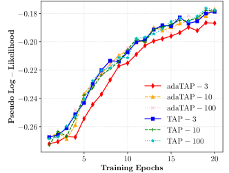
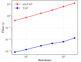
Figure 10: Left: Evolution of the pseudo-likelihood along the training of an RBM with 784 binary visible units and 500 binary hidden units. Training was performed using the 5000 first images of binarized MNIST, with a learning rate of 0.001 and batches of size 100. The different curves correspond to different strategies of estimation of the likelihood gradients, either with TAP or adaTAP. Both algorithms were iterated for a fixed number of times (3, 10 and 100). In all cases, a damping of 0.5 was used. All methods yield comparable results in terms of training performance, except for adaTAP with only 3 iterations, which shows poorer performance. Right: Computation time for one iteration of the inference algorithm, as a function of batch size. Time is reported in seconds for identical experimental settings. The need for a matrix inversion for each batch element makes VAMP 3 orders of magnitude slower than TAP.

The computational burden of Alg. 3 lies in the matrix inversion needed to evaluate $C_{2}$, which needs to be performed at each iteration. In Fig. 10 (right), we compare the time needed to perform one iteration of both the algorithms under identical experimental conditions.

This larger cost per-iteration should be compensated in principle by a more accurate inference procedure. However, that does not seem to translate to improvements in the training performance. Fig. 10 (left) presents a minimal test on 5000 MNIST training samples, where performances are reported in terms of the pseudo-likelihood. We evaluate both algorithms for different numbers of iterations. Results suggest that all strategies are roughly equivalent, except for running adaTAP for a very small number of iterations, which always leads to a poorer result.

We thus conclude that, as far as proposing a tractable and efficient training algorithm for RBMs, the TAP inference seems to serve the purpose more appropriately.

Appendix E Deep Boltzmann Machines

E.1 Model and Inference

It is possible to define as well deep models of Boltzmann machines by considering several stacked hidden layers. These Deep Boltzmann Machines (DBM) Salakhutdinov and Hinton (2009) consist in a straightforward extension of RBMs. The distribution corresponding to a DBM with $L$ hidden layers indexed by $l$ is

$$P(\mathbf{x},\mathbf{h}^{(1)},..,\mathbf{h}^{(L)};W^{(1)},..,W^{(L)},\bm{\theta}) =\frac{1}{\mathcal{Z}\left[W^{(1)},..,W^{(L)},\bm{\theta}\right]}e^{\sum_{i,j}x_{i}W_{ij}h^{(1)}_{j}+\sum_{l}\sum_{i,j}h^{(l)}_{i}W_{ij}^{(l)}h_{j}^{(l+1)}}$$

$$\quad\times\prod_{i}P_{i}^{\rm v}(x_{i};\theta_{i}^{\rm v})\prod_{l}\prod_{j}P_{j}^{\mathrm{h}(l)}(h_{j}^{(l)};{\theta_{j}^{\rm h}}^{(l)}).$$ (119)

Similarly to RBMs, the distribution of visible variables is obtained by marginalizing out the latent variables,

$$P(\mathbf{x};W^{(1)},..,W^{(L)},\bm{\theta})=\int\left(\prod_{l}\prod_{j}{\rm d}h^{(l)}_{j}\right)P(\mathbf{x},\mathbf{h}^{(1)},..,\mathbf{h}^{(L)};W^{(1)},..,W^{(L)},\bm{\theta}),$$ (120)

yielding the following log-likelihood

$$\ln P(\mathbf{x};W^{(1)},..,W^{(L)},\bm{\theta}) =-\ln\mathcal{Z}\left[W^{(1)},..,W^{(L)},\bm{\theta}\right]+\sum_{i}\ln P_{i}(x_{i};\theta_{i}^{\rm v})$$

$$\quad+\ln\int\left(\prod_{l}\prod_{j}{\rm d}h^{(l)}_{j}\right)e^{\sum_{i,j}x_{i}W_{ij}h^{(1)}_{j}+\sum_{l}\sum_{i,j}h^{(l)}_{i}W_{ij}^{(l)}h_{j}^{(l+1)}}\prod_{l}\prod_{j}P_{j}^{\mathrm{h}(l)}(h_{j}^{(l)};{\theta_{j}^{\rm h}}^{(l)}).$$ (121)

The major difference between RBMs and DBMs lies in the complexity of evaluating the above expression. Whereas for RBMs only the log-partition features a problematic multidimensional integral Eq. (11), here both the log-partition and the last term are intractable. This additional complication carries through to the computation of the gradients necessary for training, since the data-dependent term deriving from the last term of (121) is no longer tractable.

This intractability follows from the fact that hidden units in neighboring layers are now connected to each other, and are thus no longer conditionally independent. Interestingly, the first proposal to deal with the data-dependent terms of DBMs consisted in using a naive mean-field approximation Salakhutdinov and Hinton (2009), while keeping a Monte Carlo based strategy to compute gradients deriving from the log-partition. In this work, we propose instead to use the TAP approximation for both of them, hence improving on the NMF approximation and avoiding any sampling of the rather complicated RBMs.

The TAP equations related to the log-partition $\mathcal{Z}\left[W^{(1)},..,W^{(L)},\bm{\theta}\right]$ follow directly from the general derivation of Sec. V for fully connected models, with however a different weight matrix being used. For instance, the effective weight matrix of a DBM with 2 hidden layers is defined by blocks as

$$W=\left(\begin{array}[]{ccc}0&W^{(1)}&0\\ {W^{(1)}}^{T}&0&W^{(2)}\\ 0&{W^{(2)}}^{T}&0\\ \end{array}\right).$$ (125)

Thus, implementing the GRBM inference algorithm Alg. 1 with the proper weights outputs TAP solutions $\{\mathbf{a},\mathbf{c},\mathbf{B},\mathbf{A}\}$, each of them a vector with components corresponding to the different units in the DBM.

For the last term of (121), we recognize the log-partition of a model closely related to the considered DBM, where visible units are not anymore variable but fixed, or clamped, at values $x_{i}$, and the original interaction between visible and first hidden layer units is replaced by an additional local field on each $h^{(1)}_{j}$ equal to $\sum_{i}W_{ij}^{(1)}x_{i}$. Finally, under this simple modification of the Hamiltonian, TAP equations follow again from the general derivation in Sec. V. The resultant TAP solutions depending on data points $\mathbf{x}$ are said to be clamped and denoted as $\{\mathbf{\bar{a}(x)},\mathbf{\bar{c}(x)},\mathbf{\bar{B}(x)},\mathbf{\bar{A}(x)}\}$.

E.2 Training Algorithm and Experiments

The gradients of the log-likelihood with respect to the model parameters $\bm{\theta}$ are similar to the RBM ones, given by (12), (13) and (14). However, the first data-dependent term cannot be analytically computed anymore, and we use the clamped TAP solutions to approximate it. The second term is evaluated using the data-independent TAP solutions, similarly to our strategy for RBMs. The corresponding expressions of the gradients are

$$\Delta\theta_{i}^{\rm v}\approx\frac{1}{M} \sum_{m}\frac{\partial}{\partial\theta_{i}^{\rm v}}\left[\ln P_{i}^{\rm v}(x_{i}^{(m)};\theta_{i}^{\rm v})\right]$$

$$-\frac{1}{K} \sum_{k}\frac{\partial}{\partial\theta_{i}^{\rm v}}\left[\ln Z_{i}^{\rm v}(B_{i,k}^{\rm v},A_{i,k}^{\rm v};\theta_{i}^{\rm v})\right]\,,$$ (126)

$$\Delta{\theta_{j}^{\rm h}}^{(l)}\approx\frac{1}{M} \sum_{m}\frac{\partial}{\partial{\theta_{j}^{\rm h}}^{(l)}}\Big{[}$$

$$\quad\quad\quad\ln Z_{j}^{\rm h}(\bar{B}_{j}^{\rm h}(\mathbf{x}^{(m)}),\bar{A}_{j}^{\rm h}(\mathbf{x}^{(m)});{\theta_{j}^{\rm h}}^{(l)})\Big{]}$$

$$-\frac{1}{K} \sum_{k}\frac{\partial}{\partial{\theta_{j}^{\rm h}}^{(l)}}\left[\ln Z_{j}^{\rm h}(B_{j,k}^{\rm h},A_{j,k}^{\rm h};{\theta_{j}^{\rm h}}^{(l)})\right],$$ (127)

$$\Delta W^{(1)}_{ij}\approx\frac{1}{M} \sum_{m}x_{i}^{(m)}\bar{a}_{j}^{\rm h^{(1)}}(\mathbf{x}^{(m)})$$

$$-\frac{1}{K} \sum_{k}\left\{a_{i,k}^{\rm v}a_{j,k}^{\rm h^{(1)}}+W_{ij}^{(1)}c_{i,k}^{\rm v}c_{j,k}^{\rm h^{(1)}}\right\},$$ (128)

$$\Delta W^{(l)}_{ij}\approx\frac{1}{M} \sum_{m}\left\{\bar{a}_{i}^{\rm h^{(l-1)}}(\mathbf{x}^{(m)})\bar{a}_{j}^{\rm h^{(l)}}(\mathbf{x}^{(m)})\right.$$

$$\left.\quad\quad+W_{ij}^{(l)}\bar{c}_{i}^{\rm h^{(l-1)}}(\mathbf{x}^{(m)})\bar{c}_{j}^{\rm h^{(l)}}(\mathbf{x}^{(m)})\right\}$$

$$-\frac{1}{K} \sum_{k}\left\{a_{i,k}^{\rm h^{(l-1)}}a_{j,k}^{\rm h^{(l)}}+W_{ij}^{(l)}c_{i,k}^{\rm h^{(l-1)}}c_{j,k}^{\rm h^{(l)}}\right\}\text{ for }l\geq 2\,.$$ (129)

These expressions can be plugged to a gradient ascent algorithm, as in the RBM training algorithm Alg. 2. Nevertheless, this simple strategy of simultaneous training of all the parameters of the model (joint training) usually fails as the magnitude of weights of deep layers typically remains very small and the model eventually resembles a mere RBM. Several regularizations have been proposed to tackle this well-known problem of DBM training Salakhutdinov and Hinton (2009); Salakhutdinov and Larochelle (2010); Montavon and Müller (2012); Desjardins et al. (2012); Melchior et al. (2016). In our experiments, we used a greedy layerwise pre-training Salakhutdinov and Hinton (2009), which consists in computing a meaningful initialization of the weights by training the RBMs layer-by-layer, before performing the joint training. The complete algorithm is described in Alg. 4.

Fig. 11 shows the evolution of the TAP log-likelihood for a 2-hidden layer and a 3-hidden layer DBMs, trained with the above described algorithm.

Algorithm 3 AdaTAP inference for binary-binary RBMs

  Input: $J$, $\mathbf{H}$

  Initialize: $t=0$, $\mathbf{A_{1}}^{\rm(0)}$, $\mathbf{B_{1}}^{\rm(0)}$

  repeat

     Prior Updates 

     $a_{1,i}^{(t+1)}={\rm sigm}(B_{1,i}^{(t)}-A_{1,i}^{(t)}/2)$

     $c_{1,i}^{(t+1)}=a_{1,i}^{(t+1)}(1-a_{1,i}^{(t+1)})$

     $A_{2,i}^{(t+1)}=1/c_{1,i}^{(t+1)}-A_{1,i}^{(t+1)}$

     $B_{2,i}^{(t+1)}=1/(1-a_{1,i}^{(t+1)})-B_{1,i}^{(t+1)}$

     

     Interaction Updates 

     $C_{2}^{(t+1)}=(\operatorname{diag}(A_{2}^{(t+1)})-J)^{-1}$

     $a_{2,i}^{(t+1)}=\displaystyle\sum_{j}\left(C_{2}^{(t+1)}\right)_{ij}\left(B_{2,j}^{(t+1)}+H_{j}\right)$

     $A_{1,i}^{(t+1)}=1/\left(C_{2}^{(t+1)}\right)_{ii}-A_{2,i}^{(t+1)}$

     $B_{1,i}^{(t+1)}=a_{2,i}^{(t+1)}/\left(C_{2}^{(t+1)}\right)_{ii}-B_{2,i}^{(t+1)}$

     $t=t+1$

  until Convergence

Algorithm 4 GDBM Training

  Input: $\mathbf{X}$, $T_{\rm pretrain}$,$T_{\rm joint\;train}$, $M$, $K$, $R(\cdot)$

  Pretraining 

  $W^{(1)},\bm{\theta}^{\rm v},\bm{\theta}^{\mathrm{h}^{(1)}}\leftarrow$ Alg. 2($\mathbf{X}$, $T_{\rm pretrain}$, $M$, $K$, $R(\cdot)$)

  for All hidden layers $l\geq 2$ do

     $\mathbf{H}^{(l-1)}\sim P\left(\mathbf{h}^{(l)}|\mathbf{H}^{(l-1)},...,\mathbf{H}^{1},\mathbf{X}\right)$

     $W^{(l)},\bm{\theta}^{\mathrm{h}^{(l)}}\leftarrow$ Alg. 2($\mathbf{H}^{(l-1)}$, $T_{\rm pretrain}$, $M$, $K$, $R(\cdot)$)

  end for

  Joint training 

  Initialize: t = 0

  repeat

     for All mini-batches $\mathbf{X}^{B}$ of size $M$ do

        $\mathbf{a}^{(t+1)},\mathbf{c}^{(t+1)},\mathbf{B}^{(t+1)},\mathbf{A}^{(t+1)}\leftarrow$ Alg. 1$(W^{(t)},\bm{\theta}^{(t)})\times K$

        $\mathbf{\bar{a}}^{(t+1)},\mathbf{\bar{c}}^{(t+1)},\mathbf{\bar{B}}^{(t+1)},\mathbf{\bar{A}}^{(t+1)}\leftarrow$ Alg. 1$(\mathbf{X}^{B},W^{(t)},\bm{\theta}^{(t)})$

        $W_{ij}^{(l),(t+1)}\leftarrow W_{ij}^{(l),(t)}+\gamma\Delta W_{ij}^{(l),(t)}$

        ${\theta_{j}^{\rm h}}^{(l),(t+1)}\leftarrow{\theta_{j}^{\rm h}}^{(l),(t)}+\gamma\Delta{\theta_{j}^{\rm h}}^{(l),(t)}$

        ${\theta_{i}^{\rm v}}^{,(t+1)}\leftarrow{\theta_{i}^{\rm v}}^{,(t)}+\gamma\Delta{\theta_{i}^{\rm v}}^{,(t)}$

     end for

     $t\leftarrow t+1$

  until $t>T_{\rm joint\;train}$

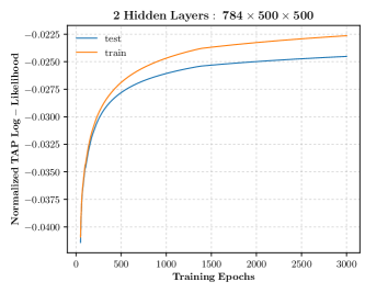
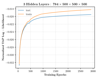
Figure 11: Training performances over 3000 training epochs for a 2-hidden layer (left) and 3-hidden layer (right) deep Boltzmann machines (DBMs) on the binarized MNIST datasets. Both models were pretrained for 50 epochs with the same learning rate of 0.001. The training performance is measured as the normalized (per unit) TAP log-likelihood for the test images (blue) and the train images (orange).

Appendix F Comparison of the TAP log-likelihood with other surrogates

As detailed in the main text, we consider the TAP log-likelihood as a surrogate to the true and intractable log-likelihood, as there are no guarantees to how close it lies to the true value, nor does it provide any bound on the value of the true log-likelihood – as discussed in Section V.2, the TAP estimate may fall either above or below. Surrogates, such as the pseudo-likelihood Besag (1975), are widely used in Boltzmann machine learning Tieleman (2008).As a surrogate for the true log-likelihood, besides its fast convergence and deterministic calculation, the TAP log-likelihood possesses many interesting properties which we study in our experiments. For instance, TAP machines can be used for denoising, as demonstrated in Section VII.4, or as priors for other applications of statistical inference.

Another piece of supporting evidence for the quality of the TAP log-likelihood as a surrogate comes from studying how consistent it is with other estimators and surrogates. We present two of them here: the pseudo-likelihood (PL), and the log-likelihood estimate provided by annealed importance sampling (AIS) Neal (2001). For this experiment, we compare log-likelihood estimates from TAP, PL, and AIS over the course of 100 epochs of training performed on a single binary-binary RBM with 500 hidden units using the binary-MNIST dataset as training data. The training is performed by maximizing the TAP log-likelihood, and each of the three approaches produces either an estimate or a surrogate to the true log-likelihood at the end of each epoch (as in Fig. 3(a)). We show the comparison of these surrogates over training in Fig. 12.

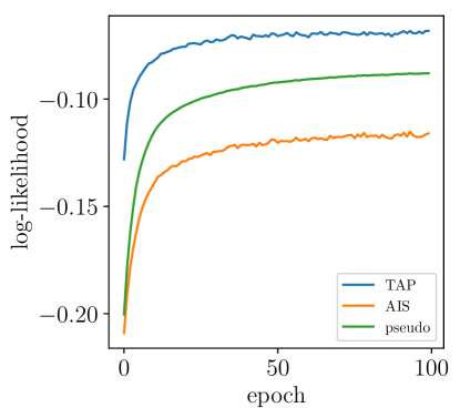
Figure 12: Comparison of the TAP log-likelihood to two other measures: the estimate provided by annealed importance sampling (AIS) and the (log) pseudo-likelihood (PL). All three measures are evaluated for the same sets of parameters, which correspond to the training of a binary-binary RBM using the TAP log-likelihood (see Fig. 3(a)). The AIS results are averaged over 100 runs. For each run, 14,500 intermediate distributions are generated between the initial and target distribution using the same schedule as in Salakhutdinov (2008). The pseudo-likelihood is computed using a stochastic approximation over 100 of the 784 pixels. Even though the training is performed so as to maximize the TAP log-likelihood, the AIS and PL estimates also increase, indicating the measures to be consistent.

All three measures have the same qualitative behavior as a function of epochs, indicating they are consistent to each other in this particular experiment. Notably, over training, one does not need to accurately estimate the value of the underlying true log-likelihood, but rather provide the same quality as a metric, that is, if one set of model parameters has a larger log-likelihood than another according to the true log-likelihood, then it should also be larger in the surrogate. As long as the “landscape” of the log-likelihood is preserved by the surrogate, then it should be sufficient for training accurate models. While the true log-likelihood is unknowable in the context of this experiment, comparing to the AIS estimate shows similar growth in log-likelihood between the TAP surrogate and AIS. Thus, we can observe that maximizing the TAP log-likelihood does indeed appear to produce models which improve the true log-likelihood overtraining, indicating some correspondence between the TAP log-likelihood and the true log-likelihood, up to the AIS estimate.

References

- LeCun et al. (2015) Y. LeCun, Y. Bengio, and G. Hinton, Deep learning, Nature 521, 436 (2015).
- Hopfield (1982) J. J. Hopfield, Neural networks and physical systems with emergent collective computational abilities, Proc. Nat. Acad. Sci. U.S.A. 79, 2254 (1982).
- Amit et al. (1985) D. J. Amit, H. Gutfreund, and H. Sompolinsky, Numbers of patterns in a spin-glass model of neural networks, Phys. Rev. Lett. 55, 1530 (1985).
- Ackley et al. (1985) D. H. Ackley, G. E. Hinton, and T. J. Sejnowski, A learning algorithm for Boltzmann machines, Cognitive Science 9, 147 (1985).
- Mézard et al. (1987) M. Mézard, G. Parisi, and M. A. Virasoro, Spin glass theory and beyond, World Scientific Lecture notes in Physics, Vol. 9 (World Scientific, 1987).
- Sessak and Monasson (2009) V. Sessak and R. Monasson, Small-correlation expansions for the inverse Ising problem, J. Phys. A 42, 055001 (2009).
- Ricci-Tersenghi (2012a) F. Ricci-Tersenghi, The Bethe approximation for solving the inverse Ising problem: a comparison with other inference methods, J. Stat. Mech. 2012, P08015 (2012a).
- Ekeberg et al. (2013) M. Ekeberg, C. Lövkvist, Y. Lan, M. Weigt, and E. Aurell, Improved contact prediction in proteins: using pseudolikelihoods to infer Potts models, Phys. Rev. E 87, 012707 (2013).
- Hinton (2002) G. Hinton, Training products of experts by minimizing contrastive divergence, Neural Comp. 14, 1771 (2002).
- Hinton and r. salakhutdinov (2006) G. Hinton and r. salakhutdinov, Reducing the dimensionality of data with neural networks, Science 313, 504 (2006).
- Larochelle and Bengio (2008) H. Larochelle and Y. Bengio, Classification using discriminative restricted Boltzmann machines, in Proc. Int. Conf. on Machine Learning (2008) pp. 536–543.
- Salakhutdinov et al. (2007) R. Salakhutdinov, A. Mnih, and G. Hinton, Restricted Boltzmann machines for collaborative filtering, in Proc. Int. Conf. on Machine Learning (2007) pp. 791–798.
- Coates et al. (2011) A. Coates, A. Y. Ng, and H. Lee, An analysis of single-layer networks in unsupervised feature learning, in Proc. Int. Conf. on Art. Intel. and Stat. (2011) pp. 215–223.
- Hinton and Salakhutdinov (2009) G. Hinton and R. Salakhutdinov, Replicated softmax: an undirected topic model, in Adv. in Neural Info. Processing Sys. (2009) pp. 1607–1614.
- Hinton et al. (2006) G. Hinton, S. Osindero, and Y.-W. Teh, A fast learning algorithm for deep belief nets, Neural Comp. 18, 1527 (2006).
- Salakhutdinov and Larochelle (2010) R. Salakhutdinov and H. Larochelle, Efficient learning of deep Boltzmann machines, in Proc. Int. Conf. on Art. Intel. and Stat. (2010) pp. 693–700.
- Goodfellow et al. (2016) I. Goodfellow, Y. Bengio, and A. Courville, Deep Learning (MIT Press, 2016) http://www.deeplearningbook.org.
- Tieleman (2008) T. Tieleman, Training restricted Boltzmann machines using approximations to the likelihood gradient, in Proc. Int. Conf. on Machine Learning (2008) pp. 1064–1071.
- Neal (2001) R. M. Neal, Annealed importance sampling, Stat. Comp. 11, 125 (2001).
- Salakhutdinov and Murray (2008) R. Salakhutdinov and I. Murray, On the quantitative analysis of deep belief networks, in Proc. Int. Conf. on Machine Learning (2008) pp. 872–879.
- Burda et al. (2015) Y. Burda, R. B. Grosse, and R. Salakhutdinov, Accurate and conservative estimates of MRF log-likelihood using reverse annealing, in Proc. Int. Conf. on Art. Intel. and Stat., Vol. 38 (2015) pp. 102–110.
- Schulz et al. (2010) H. Schulz, A. Müller, and S. Behnke, Investigating convergence of restricted Boltzmann machine learning, in Deep Learning and Unsupervised Feature Learning, NIPS Workshop on (Whistler, CA, 2010).
- Thouless et al. (1977) D. J. Thouless, P. W. Anderson, and R. G. Palmer, Solution of ‘Solvable model of a spin glass’, Philos. Mag. 35, 593 (1977).
- Opper and Winther (1997) M. Opper and O. Winther, A mean field algorithm for bayes learning in large feedforward neural networks, in Adv. in Neural Info. Processing Sys., Vol. 9 (1997) pp. 225–231.
- Bachschmid-Roman et al. (2016) L. Bachschmid-Roman, C. Battistin, M. Opper, and Y. Roudi, Variational perturbation and extended Plefka approaches to dynamics on random networks: the case of the kinetic Ising model, J. Phys. A 49, 434003 (2016).
- Salakhutdinov and Hinton (2009) R. Salakhutdinov and G. Hinton, Deep Boltzmann machines, in Proc. Int. Conf. on Art. Intel. and Stat. (2009) pp. 448–455.
- Smolensky (1986) P. Smolensky, Information processing in dynamical systems: Foundations of harmony theory, (MIT Press, 1986).
- Desjardins et al. (2010) G. Desjardins, A. Courville, Y. Bengio, P. Vincent, and O. Delalleau, Parallel tempering for training of restricted Boltzmann machines, (2010) pp. 145–152.
- Salakhutdinov (2010) R. Salakhutdinov, Learning in Markov random fields using tempered transitions, Adv. in Neural Info. Processing Sys. 23, 1 (2010).
- Bengio et al. (2007) Y. Bengio, P. Lamblin, D. Popovici, and H. Larochelle, Greedy layer-wise training of deep networks, Adv. in Neural Info. Processing Sys. 19, 153 (2007).
- Cho (2011) K. Cho, Improved learning algorithms for restricted Boltzmann machines, Learning , 10 (2011).
- Welling et al. (2004) M. Welling, M. Rosen-Zvi, and G. E. Hinton, Exponential family harmoniums with an application to information retrieval, in Adv. in Neural Info. Processing Sys. (2004) pp. 1481–1488.
- Fischer and Igel (2010) A. Fischer and C. Igel, Empirical analysis of the divergence of Gibbs sampling based learning algorithms for restricted Boltzmann machines, (2010) pp. 1–10.
- Plefka (1982) T. Plefka, Convergence condition of the TAP equation for the infinite-ranged Ising spin glass model, J. Phys. A 15, 1971 (1982).
- Georges and Yedidia (1999) A. Georges and J. S. Yedidia, How to expand around mean-field theory using high-temperature expansions, J. Phys. A 24, 2173 (1999).
- Yedidia (2001) J. Yedidia, in Advanced Mean Field Methods: Theory and Practice (MIT Press, 2001) pp. 21–36.
- Zamponi (2010) F. Zamponi, Mean field theory of spin glasses, (2010).
- Welling and Hinton (2002) M. Welling and G. Hinton, A new learning algorithm for mean field Boltzmann machines, in Proc. Int. Conf. on Art. Neural Networks (2002) pp. 351–357.
- Kappen and Rodríguez (1998) H. J. Kappen and F. B. Rodríguez, Efficient learning in Boltzmann machines using linear response theory, Neural Comp. 10, 1137 (1998).
- Gabrié et al. (2015) M. Gabrié, E. W. Tramel, and F. Krzakala, Training restricted Boltzmann machines via the Thouless-Andreson-Palmer free energy, in Adv. in Neural Info. Processing Sys. (2015) pp. 640–648.
- Welling and Teh (2003) M. Welling and Y. W. Teh, Approximate inference in Boltzmann machines, Art. Int. 143, 19 (2003).
- Tramel et al. (2016) E. W. Tramel, A. Drémeau, and F. Krzakala, Approximate message passing with restricted Boltzmann machine priors, J. Stat. Mech. 2016, 073401 (2016).
- Ricci-Tersenghi (2012b) F. Ricci-Tersenghi, The Bethe approximation for solving the inverse Ising problem: a comparison with other inference methods, J. Stat. Mech. 2012, P08015 (2012b).
- Mézard (2016) M. Mézard, Mean-field message-passing equations in the Hopfield model and its generalizations, (2016), arXiv preprint [cond-mat.dis-nn]:1608.01558.
- Courville et al. (2011) A. Courville, J. Bergstra, and Y. Bengio, A spike and slab restricted Boltzmann machine, in Proc. Int. Conf. on Art. Intel. and Stat., Vol. 15 (2011).
- Pearl (1982) J. Pearl, Reverend Bayes on inference engines: A distributed hierarchical approach, in Proc. AAAI Conf. on Art. Int. (1982) pp. 133–136.
- Yedidia and amd Yair Weiss (2001) J. S. Yedidia and W. T. F. amd Yair Weiss, Bethe free energy, Kikuchi approximations, and belief propagation algorithms, in Adv. in Neural Info. Processing Sys., Vol. 13 (2001).
- Huang and Toyoizumi (2015) H. Huang and T. Toyoizumi, Advanced mean-field theory of the restricted Boltzmann machine, Phys. Rev. E 91, 050101 (2015).
- Sudderth et al. (2010) E. B. Sudderth, A. T. Ihler, M. Isard, W. T. Freeman, and A. S. Willsky, Nonparametric belief propagation, Commun. ACM 53, 95 (2010).
- Opper and Winther (2005) M. Opper and O. Winther, Expectation consistent approximate inference, J. Machine Learning Resaerch 6, 2177 (2005).
- Rangan (2010) S. Rangan, Estimation with random linear mixing, belief propagation and compressed sensing, in Proc. Annual Conf. on Info. Sci. and Sys. (2010) pp. 1–6.
- Lesieur et al. (2015a) T. Lesieur, F. Krzakala, and L. Zdeborová, Phase transitions in sparse PCA, in Proc. IEEE Int. Symp. on Info. Theory (2015) pp. 1635–1639.
- Lesieur et al. (2015b) T. Lesieur, F. Krzakala, and L. Zdeborová, MMSE of probabilistic low-rank matrix estimation: Universality with respect to the output channel, in Proc. Allerton Conf. on Communication, Control, and Computing (2015) pp. 680–687.
- Deshpande and Montanari (2014) Y. Deshpande and A. Montanari, Information-theoretically optimal sparse PCA, in Proc. IEEE Int. Symp. on Info. Theory (2014) pp. 2197–2201.
- Rangan and Fletcher (2012) S. Rangan and A. K. Fletcher, Iterative estimation of constrained rank-one matrices in noise, in Proc. IEEE Int. Symp. on Info. Theory (2012) pp. 1246–1250.
- Lesieur et al. (2017) T. Lesieur, F. Krzakala, and L. Zdeborová, Constrained low-rank matrix estimation: Phase transitions, approximate message passing and applications, J. Stat. Mech. 2017, 073403 (2017).
- Opper and Winther (2001) M. Opper and O. Winther, Tractable approximations for probabilistic models: The adaptive Thouless-Anderson-Palmer mean field approach, Phys. Rev. Lett. 86, 3695 (2001).
- Yedidia (2000) J. S. Yedidia, An idiosyncratic journey beyond mean field theory, (MIT Press, 2000).
- Wainwright and Jordan (2008) M. J. Wainwright and M. I. Jordan, Graphical Models, Exponential Families, and Variational Inference, Foundations and Trends in Machine Learning, Vol. 1 (Now Publishers Inc., 2008).
- Dominicis and Young (1983) C. D. Dominicis and A. P. Young, Weighted averages and order parameters for the infinite range Ising spin glass, J. Phys. A 16, 2063 (1983).
- Mézard and Montanari (2009) M. Mézard and A. Montanari, Information, Physics, and Computation (Oxford University Press, 2009).
- Krzakala et al. (2012) F. Krzakala, M. Mézard, F. Sausset, Y. Sun, and L. Zdeborová, Probabilistic reconstruction in compressed sensing: Algorithms, phase diagrams, and threshold achieving matrices, J. Stat. Mech. 2012, P08009 (2012).
- LeCun et al. (1998) Y. LeCun, L. Bottou, Y. Bengio, and P. Haffner, Gradient-based learning applied to document recognition, Proc. IEEE 86, 2278 (1998).
- MIT Center For Biological and Computation Learning (2000) MIT Center For Biological and Computation Learning, CBCL face database #1, (2000).
- Cho et al. (2013) K. Cho, T. Raiko, and A. Ilin, Enhanced gradient for training restricted boltzmann machines, Neural Comp. 25, 805 (2013).
- Tenenbaum et al. (2000) J. B. Tenenbaum, V. de Silva, and J. C. Langford, A global geometric framework for nonlinear dimensionality reduction, Science 290, 2319 (2000).
- Şendur and Selesnick (2002) L. Şendur and I. W. Selesnick, Bivariate shrinkage functions for wavelet-based denoising exploiting interscale dependency, IEEE Trans. Sig. Processing 50, 2744 (2002).
- van Ginneken and Mendrik (2006) B. van Ginneken and A. Mendrik, Image denoising with -nearest neighbor and support vector regression, in Proc. Int. Conf. on Pattern Recognition (2006).
- Melchior et al. (2017) J. Melchior, N. Wang, and L. Wiskott, Gaussian-binary restricted Boltzmann machines on modeling natural image statistics, PLOS ONE 12, e0171015 (2017).
- Cho et al. (2011) K. Cho, A. Ilin, and T. Raiko, Improved learning of gaussian-bernoulli restricted Boltzmann machine, in Proc. Int. Conf. on Art. Neural Networks (2011) pp. 10–17.
- Tubiana and Monasson (2016) J. Tubiana and R. Monasson, Emergence of compositional representations in restricted Boltzmann machines, (2016), arXiv preprint [physics.data-an]:1611.06759.
- Barra et al. (2016) A. Barra, G. Genovese, P. Sollich, and D. Tantari, Phase transitions in restricted Boltzmann machines with generic priors, (2016), arXiv preprint [cond-mat.dis-nn]:1612.03132.
- Rangan et al. (2017) S. Rangan, P. Schniter, and A. K. Fletcher, Vector approximate message passing, in Information Theory (ISIT), 2017 IEEE International Symposium on (2017) pp. 1588–1592.
- Montavon and Müller (2012) G. Montavon and K. R. Müller, in Neural Networks: Tricks of the Trade (Springer, 2012) pp. 621–637.
- Desjardins et al. (2012) G. Desjardins, A. Courville, and Y. Bengio, On Training Deep Boltzmann Machines, (2012), arXiv preprint [cs.NN]:1203.4416.
- Melchior et al. (2016) J. Melchior, A. Fischer, and L. Wiskott, How to center deep boltzmann machines, J. Machine Learning Resaerch 17, 1 (2016).
- Besag (1975) J. Besag, Statistical analysis of non-lattice data, The statistician , 179 (1975).
- Salakhutdinov (2008) R. Salakhutdinov, MATLAB code for AIS, http://www.utstat.toronto.edu/~rsalakhu/rbm_ais.html (2008).