Fast and Compact Exact Distance Oracle for Planar Graphs

Abstract

For a given a graph, a distance oracle is a data structure that answers distance queries between pairs of vertices. We introduce an $O(n^{5/3})$-space distance oracle which answers exact distance queries in $O(\log n)$ time for $n$-vertex planar edge-weighted digraphs. All previous distance oracles for planar graphs with truly subquadratic space (i.e., space $O(n^{2-\epsilon})$ for some constant $\epsilon>0$) either required query time polynomial in $n$ or could only answer approximate distance queries.

Furthermore, we show how to trade-off time and space: for any $S\geq n^{3/2}$, we show how to obtain an $S$-space distance oracle that answers queries in time $O(\frac{n^{5/2}}{S^{3/2}}\log n)$. This is a polynomial improvement over the previous planar distance oracles with $o(n^{1/4})$ query time.

1 Introduction

Efficiently storing distances between the pairs of vertices of a graph is a fundamental problem that has receive a lot of attention over the years. Many graph algorithms and real-world problems require that the distances between pairs of vertices of a graph can be accessed efficiently. Given an edge-weighted digraph $G=(V,E)$ with $n$ vertices, a distance oracle is a data structure that can efficiently answer distance queries between pairs of vertices $u,v\in V$.

A naive approach consists in storing an $n\times n$ distance matrix, giving a distance query time of $O(1)$ by a simple table lookup. The obvious downside is the huge $\Theta(n^{2})$ space requirement which is in many cases impractical. For example, several popular routing heuristics (e.g.: for the travelling salesman problem) require fast access to distances between pairs of vertices. Unfortunately the inputs are usually too big to allow to store an $n\times n$ distance matrix (see e.g.: [1]).

Fast and compact data structures for distances are also critical in many routing problems. One important challenge in these applications is to process a large number of online queries while keeping the space usage low, which is important for systems with limited memory or memory hierarchies. Therefore, the alternative naive approach consisting in simply storing the graph $G$ and answering a query by running a shortest path algorithm on the entire graph is also prohibitive for many applications.

Since road networks and planar graphs share many properties, planar graphs are often used for modeling various transportation networks (see e.g.: [26]). Therefore obtaining good space/query-time trade-offs for planar distance oracles has been studied thoroughly over the past decades [10, 3, 8, 12, 30, 4, 26].

If $S$ represents the space usage and $Q$ represents the query time, the trivial solutions described above would suggest a trade-off of $Q=n^{2}/S$. Up to logarithmic factors, this trade-off is achieved by the oracles of Djidjev [10] and Arikati, et al. [3]. The oracle of Djidjev further improves on this trade-off obtaining an oracle with $Q=n/\sqrt{S}$ for the range $S\in[n^{4/3},n^{3/2}]$ suggesting that this trade-off might instead be the correct one. Extending this trade-off to the full range of $S$ was the subject of several subsequent papers by Chen and Xu [8], Cabello [4], Fakcharoenphol and Rao [12], and finally Mozes and Sommer [26] (see also the result of Nussbaum [27]) obtaining a query time of $Q=n/\sqrt{S}$ for the entire range of $S\in[n,n^{2}]$ (again ignoring constant and logarithmic factors).

It is worth noting that the above mentioned trade-off between space usage and query time is no better than the trivial solution of simply storing the $n\times n$ distance matrix when constant (or even polylogarithmic) query time is needed. In fact the best known result in this case due to Wulff-Nilsen [30] who manages to obtain very slightly subquadratic space of $O(n^{2}\operatorname{polyloglog}(n)/\log(n))$ and constant query time. It has been a major open question whether an exact oracle with truly subquadratic (that is, $O(n^{2-\varepsilon})$ for any constant $\varepsilon>0$) space usage and constant or even polylogarithmic query time exists. Furthermore, the trade-offs obtained in the literature suggest that this might not be the case.

In this paper we break this quadratic barrier:

Theorem 1.

Let $G=(V,E)$ be a weighted planar digraph with $n$ vertices. Then there exists a data structure with $O(n^{2})$ preprocessing time and $O(n^{5/3})$ space and a data structure with $O(n^{11/6})$ space and $O(n^{11/6})$ expected preprocessing time. Given any two query vertices $u,v\in V$, both oracles report the shortest path distance from $u$ to $v$ in $G$ in $O(\log n)$ time.

In addition to Theorem 1 we also obtain a distance oracle with a trade-off between space and query time.

Theorem 2.

Let $G=(V,E)$ be a weighted planar digraph with $n$ vertices. Let $S$ denote the space, $P$ denote the preprocessing time, and $Q$ denote the query time. Then there exists planar distance oracles with the following properties:

• $P=O(n^{2})$, $S\geq n^{3/2}$, and $Q=O(\frac{n^{5/2}}{S^{3/2}}\log n)$.

• $P=S$, $S\geq n^{16/11}$, and $Q=O(\frac{n^{11/5}}{S^{6/5}}\log n)$.

In particular, this result improves on the current state-of-the-art [26] trade-off between space and query time for $S\geq n^{3/2}$. The main idea is to use two $r$-divisions, where we apply our structure from Theorem 1 to one and do a brute-force search over the boundary nodes of the other.

Recent developments

We note that the main focus of this paper is on space usage and query time, and the the preprocessing time follows directly from our proofs (and by applying the result of [5] for subquadratic time).

After posting a preliminary version of this paper on arXiv [9], the algorithm of Cabello [5] was improved by Gawrychowski et al. [15] to run in $\tilde{O}(n^{5/3})$ deterministically. As noted in [15] this also improves the preprocessing time of our Theorem 1 to $\tilde{O}(n^{5/3})$ while keeping the space usage at $O(n^{5/3})$. It is also possible to use Gawrychowski et al. to speed-up the pre-processing time of our distance oracle described in Theorem 2. This yields a distance oracle (in the notation of Theorem 2) with $P=\tilde{O}(S)$, $S\geq n^{3/2}$, and $Q=O(\frac{n^{5/2}}{S^{3/2}}\log n)$, thus eliminating entirely the need of the second bullet point of Theorem 2.

Techniques

We derive structural results on Voronoi diagrams for planar graphs when the centers of the Voronoi cells lie on the same face. The key ingredients in our algorithm are a novel and technical separator decomposition and point location structure for the regions in an $r$-division allowing us to perform binary search to find a boundary vertex $w$ lying on a shortest-path between a query pair $u,v$. These structures are applied on top of weighted Voronoi diagrams, and our point location structure relies heavily on partitioning each region into small “easy-to-handle” wedges which are shared by many such Voronoi diagrams. More high-level ideas are given in Section 3.

Our approach bears some similarities with the recent breakthrough of Cabello [5]. Cabello showed that abstract Voronoi diagrams [24, 25] studied in computational geometry combined with planar $r$-division can be used to obtain fast planar graphs algorithms for computing the diameter and wiener index. We start from Cabello’s approach of using abstract Voronoi diagrams. While Cabello focuses on developing fast algorithms for computing abstract Voronoi diagrams of a planar graph, we introduce a decomposition theorem for abstract Voronoi diagrams of planar graphs and a new data structure for point location in planar graphs.

1.1 Related work

In this paper, we focus on distance oracles that report shortest path distances exactly. A closely related area is approximate distance oracles. In this case, one can obtain near-linear space and constant or near-constant query time at the cost of a small $(1+\epsilon)$-approximation factor in the distances reported [28, 21, 19, 20, 32].

One can also study the problem in a dynamic setting, where the graph undergoes edge insertions and deletions. Here the goal is to obtain the best trade-off between update and query time. Fakcharoenphol and Rao [12] showed how to obtain $\tilde{O}(n^{2/3})$ for both updates and queries and a trade-off of $O(r)$ and $O(n/\sqrt{r})$ in general. Several follow up works have improved this result to negative edges and shaving further logarithmic factors [22, 17, 18, 14]. Furthermore, Abboud and Dahlgaard [2] have showed that improving this bound to $O(n^{1/2-\varepsilon})$ for any constant $\varepsilon>0$ would imply a truly subcubic algorithm for the All Pairs Shortest Paths (APSP) problem in general graphs.

In the seminal paper of Thorup and Zwick [29], a $(2k-1)$-approximate distance oracle is presented for undirected edge-weighted $n$-vertex general graphs using $O(kn^{1+1/k})$ space and $O(k)$ query time for any integer $k\geq 1$. Both query time and space has subsequently been improved to $O(n^{1+1/k})$ space and $O(1)$ query time while keeping an approximation factor of $2k-1$ [31, 6, 7]. This is near-optimal, assuming the widely believed and partially proven girth conjecture of Erdős [11].

2 Preliminaries and Notations

Throughout this paper we denote the input graph by $G$ and we assume that it is a directed planar graph with a fixed embedding. We assume that $G$ is connected (when ignoring edge orientations) as otherwise each connected component can be treated separately.

Section 4 will make use of the geometry of the plane and associate Jordan curves to cycle separators. Let $H$ be a planar embedded edge-weighted digraph. We use $V(H)$ to denote the set of vertices of $H$ and we denote by $H^{*}$ the dual of $H$ (with parallel edges and loops) and view it as an undirected graph. We assume a natural embedding of $H^{*}$ i.e., each dual vertex is in the interior of its corresponding primal face and each dual edge crosses its corresponding primal edge of $H$ exactly once and intersects no other edges of $G$. We let $d_{H}(u,v)$ denote the shortest path distance from vertex $u$ to vertex $v$ in $H$.

$r$-division

We will rely on the notion of $r$-division introduced by Frederickson [13] and further developed by Klein et al. [23]. For a subgraph $H$ of $G$, a vertex $v$ of $H$ is a boundary vertex if $G$ contains an edge not in $H$ that is incident to $v$. We let $\delta H$ denote the set of boundary vertices of $H$. Vertices of $V(H)\setminus\delta H$ are called internal vertices of $H$. A hole of a subgraph $H$ of $G$ is a face of $H$ that is not a face of $G$.

Let $c_{1}$ and $c_{2}$ be constants. For a number $r$, an $r$-division with few holes of (connected) graph $G$ (with respect to $c_{1},c_{2}$) is a collection $\mathcal{R}$ of subgraphs of $G$, called regions, with the following properties.

1. Each edge of $G$ is in exactly one region.

2. The number of regions is at most $c_{1}|V(G)|/r$.

3. Each region contains at most $r$ vertices.

4. Each region has at most $c_{2}\sqrt{r}$ boundary vertices.

5. Each region contains only $O(1)$ holes.

We make the simplifying assumption that each hole $H$ of each region $R$ is a simple cycle and that all its vertices belong to $\delta R$. We can always reduce to this case as follows. First, turn $H$ into a simple cycle by duplicating vertices that are visited more than once in a walk of the hole. Then for each pair of consecutive boundary vertices in this walk, add a bidirected edge between them unless they are already connected by an edge of $R$; the new edges are embedded such that they respect the given embedding of $R$. We refer to the new simple cycle obtained as a hole and it replaces the old hole $H$.

We also make the simplifying assumption that each face of a region $R$ is either a hole or a triangle and that each edge of $R$ is bidirected. This can always be achieved by adding suitable infinite-weight edges that respect the current embedding of $R$.

Non-negative weights and unique shortest paths

As mentioned earlier, we may assume w.l.o.g. that $G$ has non-negative edge weights. Furthermore, we assume uniqueness of shortest paths i.e., for any two vertices $x,y$ of a graph $G$, there is a unique path from $x$ to $y$ that minimizes the sum of the weights of its edges. This can be achieved either with random perturbations of edge weights or deterministically with a slight overhead as described in [5]; we need the shortest paths uniqueness assumption only for the preprocessing step and thus the overhead only affects the preprocessing time and not the query time of our distance oracle.

Voronoi diagrams

We now define the key notion of Voronoi diagrams. Let $G$ be a graph and $r>0$. Consider an $r$-division with few holes $\mathcal{R}$ of $G$ and a region $R\in\mathcal{R}$ and let $H$ be a hole of $R$. Let $u$ be a vertex of $G$ not in $R$.

Let $R_{H}$ be the graph obtained from $R$ by adding inside each hole $H^{\prime}\neq H$ of $R$, a new vertex in its interior and infinite-weight bidirected edges between this vertex and the vertices of $H^{\prime}$ (which by the above simplifying assumption all belong to $\delta R$), embedding the edges such that they are pairwise non-crossing and contained in $H^{\prime}$.

Some of the following definitions are illustrated in Figure 1. Consider the shortest path tree $T_{u}$ in $G$ rooted at $u$. For any vertex $x\in V(T_{u})$, define $T_{u}(x)$ to be the subtree of $T_{u}$ rooted at $x$. For each vertex $x\in V(H)$ we define the Voronoi cell of $x$ (w.r.t. $u$, $R$, and $H$) as the set of vertices of $R_{H}$ that belong to the subtree $T_{u}(x)$ and not to any subtree $T_{u}(y)$ for $y\in(V(H)-\{x\})\cap V(T_{u}(x))$. The weighted Voronoi diagram of $u$ w.r.t. $R$ and $H$ is the collection of all the Voronoi cells of the vertices in $H$. For each vertex $x\in H$ we say that its weight is the shortest path distance from $u$ to $x$ in $G$. Note that since we assume unique shortest paths and bidirectional edges, the weighted Voronoi diagram of $u$ w.r.t. $R$ and $H$ is a partition of the vertices of $R_{H}$. Furthermore, each Voronoi cell contains exactly one vertex of $H$. For any Voronoi cell $C$, we define its boundary edges to be the edges of $R_{H}$ that have exactly one endpoint in $C$. Let $B_{H}^{*}$ be the subgraph of $R_{H}^{*}$ consisting of the (dual) boundary edges over all Voronoi cells w.r.t. $u$ and $R_{H}$; we ignore edge orientations and weights so that $B_{H}^{*}$ is an unweighted undirected graph. We define $\text{Vor}_{H}(R,u)$ to be the multigraph obtained from $B_{H}^{*}$ by replacing each maximal path whose interior vertices have degree two by a single edge whose embedding coincides with the path it replaces. When $H$ is clear from context, we simply write $\mbox{Vor}({R},{u})$.

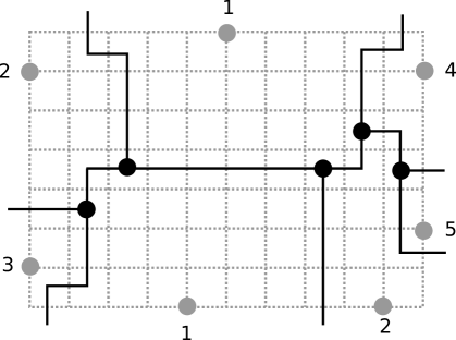
Figure 1: Illustration of the weighted Voronoi diagram of a vertex $u$ (not shown) w.r.t. a region $R$ (grey) and a hole $H$ (dotted edges and seven grey vertices). Edges of $R$ are bidirected and have weight $1$. The number next to a vertex of $H$ is the weight of that vertex. Vertices of the Voronoi diagram (which are dual vertices and hence faces of the primal) and its boundary are shown in black except the one embedded inside $H$. The graph $\text{Vor}_{H}(R,u)$ has seven edges. Note that this illustration does not have unique shortest paths as assumed in this paper. Note also that the shortest path from $u$ to the node with weight $5$ goes through the nearby node with weight $2$. Thus the rest of the shortest-path tree from $u$ has been assigned to the node with weight $5$. Note also that the illustration is not triangulated.

3 High-level description

We now give a high-level description of our distance oracle where we omit the details needed to get our preprocessing time bounds. Our data structure is constructed on top of an $r$-division of the graph. For each region $R$ of the $r$-division we store a look-up table of the distance in $G$ between each ordered pair of vertices $u,v\in V(R)$. We also store a look-up table of distances in $G$ from each vertex $u\in V$ to the boundary vertices of $R$. In total this part requires $O(nr+n^{2}/\sqrt{r})$ space.

The difficult case is when two vertices $u$ and $v$ from different regions are queried. To do this we will use weighted Voronoi diagrams. More specifically, for every vertex $u$, every region $R$, and every hole $H$ of $R$, we construct a recursive separator decomposition of the weighted Voronoi diagram of $u$ w.r.t. $R$ and $H$. The goal is to determine the boundary vertex $w$ such that $v$ is contained in the Voronoi cell of $u$. If we can do this, we know that $d_{G}(u,v)=d_{G}(u,w)+d_{R_{H}}(w,v)$ for one of the holes $H$ of $R$. To determine this we use a carefully selected recursive decomposition. This decomposition is stored in a compact way and we show how it enables binary search to find $w$ in $O(\log r)$ time.

In order to store all of the above mentioned parts efficiently we will employ the compact representation of the abstract Voronoi diagram (namely $\mbox{Vor}({R},{u})$ as defined in the previous section). This requires only $O(\sqrt{r})$ space for each choice of $u$, $R$, and $H$ for a total of $O(n^{2}/\sqrt{r})$ space. This also dominates the space for storing the recursive decompositions.

Finally, we store for each graph $R_{H}$ and each possible separator of $R_{H}$ the set of vertices on one side of the separator, since this is needed to perform the binary search. This is done in a compact way requiring only $O(r^{2})$ space per region. Thus, the total space requirement of our distance oracle is $O(nr+n^{2}/\sqrt{r})$. Picking $r=n^{2/3}$ gives the desired $O(n^{5/3})$ space bound.

4 Recursive Decomposition of Regions

In this section, we consider a region $R$ in an $r$-division of a planar embedded graph $G=(V,E)$, a vertex $u\in V-V(R)$, and a hole $H$ of $R$ which we may assume is the outer face of $R$. To simplify notation, we identify $R$ with $R_{H}$ and let $\delta R$ denote the boundary vertices of $R$ belonging to $H$, i.e., $\delta R=V(H)$ (by our simplifying assumption regarding holes in the preliminaries). The dual vertex corresponding to $H$ is denoted $v_{\infty}(R,u)$ or just $v_{\infty}$.

We assume that $R$ contains at least three boundary vertices. Recall that each face of $R$ other than the outer face is a triangle and so, each vertex of $\mbox{Vor}({R},{u})$ other than $v_{\infty}$ has degree $3$. Moreover, every cell of $\mbox{Vor}({R},{u})$ contains exactly one boundary vertex, therefore the boundary of each cell of $\mbox{Vor}({R},{u})$ contains exactly one occurrence of $v_{\infty}$ and contains at least one other vertex. Also note that the cyclic ordering of cells of $\mbox{Vor}({R},{u})$ around $v_{\infty}$ is the same as the cyclic ordering $\delta R$ of boundary vertices of $R$.

Construct a plane multigraph ${R}_{\Delta}({u})$ from $\mbox{Vor}({R},{u})$ as follows. First, for every Voronoi cell $C$, add an edge from $v_{\infty}$ to each vertex of $C$ other than $v_{\infty}$ itself; these edges are embedded such that they are fully contained in $C$ and such that they are pairwise non-crossing. For each such edge $e$, denote by $C(e)$ the cell it is embedded in. To complete the construction of ${R}_{\Delta}({u})$, remove every edge incident to $v_{\infty}$ belonging to $\mbox{Vor}({R},{u})$. The construction of ${R}_{\Delta}({u})$ is illustrated in Figure 2.

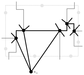
Figure 2: Illustration of ${R}_{\Delta}({u})$ highlighted in bold black edges. To avoid clutter, most edges incident to $v_{\infty}$ are only sketched.

Recursive decomposition using a Voronoi diagram

In this section, we show how to obtain a recursive decomposition of ${R}_{\Delta}({u})$ into subgraphs called pieces. A piece $Q$ is decomposed into two smaller pieces by a cycle separator $S$ of size $2$ containing $v_{\infty}$. Each of the two subgraphs of $Q$ is obtained by replacing the faces of $Q$ on one side of $S$ by a single face bounded by $S$. The separator $S$ is balanced w.r.t. the number of faces of $Q$ on each side of $S$. The recursion stops when a piece with at most six faces is obtained. It will be clear from our construction below that the collection of cycle separators over all recursive calls form a laminar family, i.e., they are pairwise non-crossing.

We assume a linked list representation of each piece $Q$ where edges are ordered clockwise around each vertex.

Lemma 2 below shows how to find the cycle separators needed to obtain the recursive decomposition into pieces. Before we can prove it, we need the following result.

Lemma 1.

Let $Q$ be one of the pieces obtained in the above recursive decomposition. Then for every vertex $v$ of $Q$ other than $v_{\infty}$,

1. $v$ has at least two edges incident to $v_{\infty}$,

2. for each edge $(v,w)$ of $Q$ where $w\neq v_{\infty}$, the edge preceding and the edge following $(v,w)$ in the clockwise ordering around $v$ are both incident to $v_{\infty}$, and

3. for every pair of edges $e_{1}=(v,v_{\infty})$ and $e_{2}=(v,v_{\infty})$ where $e_{2}$ immediately follows $e_{1}$ in the clockwise ordering around $v$, if both edges are directed from $v$ to $v_{\infty}$ then the subset of the plane to the right of $e_{1}$ and to the left of $e_{2}$ is a single face of $Q$.

Proof.

The proof is by induction on the depth $i\geq 0$ in the recursion tree of the node corresponding to piece $Q$. Assume that $i=0$ and let $v\neq v_{\infty}$ be given. The first and third part of the lemma follow immediately from the construction of ${R}_{\Delta}({u})$ and the assumption that $|\delta R|\geq 3$. To show the second part, it suffices by symmetry to consider the edge $e$ following $(v,w)$ in the cyclic ordering of edges around $v$ in $Q={R}_{\Delta}({u})$. Since $e$ and $(v,w)$ belong to the same face of $Q$ and since each face of $Q$ contains $v_{\infty}$ and at most three edges, the second part follows.

Now assume that $i>0$ and that the claim holds for smaller values. Let $v\neq v_{\infty}$ be given. Consider the parent piece $Q^{\prime}$ of $Q$ in the recursive decomposition tree and let $S$ be the cycle separator that was used to decompose $Q^{\prime}$. Then $S$ contains $v_{\infty}$ and one additional vertex $v^{\prime}$. To show the inductive step, we claim that we only need to consider the case when $v^{\prime}=v$. This is clear for the first and second part since if $v^{\prime}\neq v$ then $v$ has the same set of incident edges in $Q^{\prime}$ and in $Q$. It is also clear for the third part since $Q$ is a subgraph of $Q^{\prime}$.

It remains to show the induction step when $v^{\prime}=v$. The first part follows since the two edges of $S$ are incident to $v$ and to $v_{\infty}$ and belong to $Q$. The second part follows by observing that the clockwise ordering of edges around $v$ in $Q$ is obtained from the clockwise ordering around $v$ in $Q^{\prime}$ by removing an interval of consecutive edges in this ordering; furthermore, the first and last edge in the remaining interval are both incident to $v_{\infty}$. Applying the induction hypothesis shows the second part.

For the third part, if $e_{2}$ immediately follows $e_{1}$ in the clockwise ordering around $v$ in $Q^{\prime}$ then the induction hypothesis gives the desired. Otherwise, $e_{1}$ and $e_{2}$ must be the two edges of $S$ and $Q$ is obtained from $Q^{\prime}$ by removing the faces to the right of $e_{1}$ and to the left of $e_{2}$ and replacing them by a single face bounded by $S$. ∎

In the following, let $Q$ be a piece with more than six faces. The following lemma shows that $Q$ has a balanced cycle separator of size $2$ which can be found in $O(|Q|)$ time.

Lemma 2.

$Q$ as defined above contains a $2$-cycle $S$ containing $v_{\infty}$ such that the number of faces of $Q$ on each side of $S$ is a fraction between $1/3$ and $2/3$ of the total number of faces of $Q$. Furthermore, $S$ can be found in $O(|Q|)$ time.

Proof.

We construct $S$ iteratively. In the first iteration, pick an arbitrary vertex $v_{1}\neq v_{\infty}$ of $Q$ and let $S_{1}$ consist of two distinct arbitrary edges, both incident to $v_{1}$ and $v_{\infty}$. This is possible by the first part of Lemma 1.

Now, consider the $i$th iteration for $i>1$ and let $v_{i-1}$ and $v_{\infty}$ be the two vertices of the $2$-cycle $S_{i-1}$ obtained in the previous iteration. If $S_{i-1}$ satisfies the condition of the lemma, we let $S=S_{i-1}$ and the iterative procedure terminates.

Otherwise, one side of $S_{i-1}$ contains more than $2/3$ of the faces of $Q$. Denote this set of faces by $\mathcal{F}_{i-1}$ and let $E_{i-1}$ be the set of edges of $Q$ incident to $v_{i-1}$, contained in faces of $\mathcal{F}_{i-1}$, and not belonging to $S_{i-1}$. We must have $E_{i-1}\neq\emptyset$; otherwise, it follows from the third part of Lemma 1 that $\mathcal{F}_{i-1}$ contains only a single face of $Q$ (bounded by $S_{i-1}$), contradicting our assumption that $Q$ contains more than six faces and that $\mathcal{F}_{i-1}$ contains more than $2/3$ of the faces of $Q$.

If $E_{i-1}$ contains an edge incident to $v_{\infty}$, pick an arbitrary such edge $e_{i-1}$. This edge partitions $\mathcal{F}_{i-1}$ into two non-empty subsets; let $\mathcal{F}_{i-1}^{\prime}$ be the larger subset. We let $v_{i}=v_{i-1}$ and let $S_{i}$ be the $2$-cycle consisting of $e_{i-1}$ and the edge of $S_{i-1}$ such that one side of $S_{i}$ contains exactly the faces of $\mathcal{F}_{i-1}^{\prime}$.

Now, assume that none of the edges of $E_{i-1}$ are incident to $v_{\infty}$. Then by the second part of Lemma 1, $E_{i-1}$ contains exactly one edge $e_{i-1}$. We let $v_{i}\neq v_{i-1}$ be the other endpoint of $e_{i-1}$ and we let $S_{i}$ consist of the two edges incident to $v_{i}$ which belong to the two faces of $\mathcal{F}_{i-1}$ incident to $e_{i-1}$.

To show the first part of the lemma, it suffices to prove that the above iterative procedure terminates. Consider two consecutive iterations $i>1$ and $i+1$ and assume that the procedure does not terminate in either of these. We claim that then $\mathcal{F}_{i}\subset\mathcal{F}_{i-1}$. If we can show this, it follows that $|\mathcal{F}_{1}|>|\mathcal{F}_{2}|>\ldots$ which implies termination.

If $E_{i-1}$ contains an edge incident to $v_{\infty}$ then $\mathcal{F}_{i-1}^{\prime}$ contains more than $1/3$ of the faces of $Q$. Since the procedure does not terminate in iteration $i+1$, $\mathcal{F}_{i-1}^{\prime}$ must in fact contain more than $2/3$ of the faces so $\mathcal{F}_{i}=\mathcal{F}_{i-1}^{\prime}\subset\mathcal{F}_{i-1}$, as desired.

Now, assume that none of the edges of $E_{i-1}$ are incident to $v_{\infty}$. Then one side of $S_{i}$ contains exactly the faces of $\mathcal{F}_{i-1}$ excluding two. Since we assumed that $Q$ contains more than six faces, this side of $S_{i}$ contains more than $2/3$ of these faces. Hence, $\mathcal{F}_{i}\subset\mathcal{F}_{i-1}$, again showing the desired.

For the second part of the lemma, note that counting the number of faces of $Q$ contained in one side of a $2$-cycle containing $v_{\infty}$ can be done in the same amount of time as counting the number of edges incident to $v_{\infty}$ from one edge of the cycle to the other in either clockwise or counter-clockwise order around $v_{\infty}$. This holds since every face of $Q$ contains $v_{\infty}$. It now follows easily from our linked list representation of $Q$ with clockwise orderings of edges around vertices that the $i$th iteration can be executed in $O(|\mathcal{F}_{i-1}|-|\mathcal{F}_{i}|)$ time for each $i>1$. This shows the second part of the lemma. ∎

Corollary 1.

Given $\mbox{Vor}({R},{u})$ and ${R}_{\Delta}({u})$, its recursive decomposition can be computed in $O(\sqrt{r}\log r)$ time.

Proof.

$\mbox{Vor}({R},{u})$ has complexity $|\mbox{Vor}({R},{u})|=O(\sqrt{r})$ and ${R}_{\Delta}({u})$ can be found in time linear in this complexity. Since the recursive decomposition of ${R}_{\Delta}({u})$ has $O(\log r)$ levels and since the total size of pieces on any single level is $O(|{R}_{\Delta}({u})|)=O(|\mbox{Vor}({R},{u})|)=O(\sqrt{r})$, the corollary follows from Lemma 2. ∎

Lemma 3.

The recursive decomposition of ${R}_{\Delta}({u})$ can be stored using $O(\sqrt{r})$ space.

Proof.

Observe that the number of nodes of the tree decomposition is $O(\sqrt{r})$ and each separator consists of two edges and so takes $O(1)$ space. ∎

Embedding of ${R}_{\Delta}({u})$:

We now provide a more precise definition of the embedding of ${R}_{\Delta}({u})$. Let $f_{\infty}$ be the face of $R$ corresponding to $v_{\infty}$ in $R^{*}$, i.e., $f_{\infty}$ is the hole $H$. Consider the graph $\tilde{R}$ that consists of $R$ plus a vertex $\tilde{v}_{\infty}$ located in $f_{\infty}$ and an edge between each vertex of $f_{\infty}$ and $\tilde{v}_{\infty}$. The rest of $\tilde{R}$ is embedded consistently with respect to the embedding of $R$.

Now, consider the following embedding of ${R}_{\Delta}({u})$. First, embed $v_{\infty}$ to $\tilde{v}_{\infty}$. We now specify the embedding of each edge adjacent to $v_{\infty}$. Recall that each edge $e$ that is adjacent to $v_{\infty}$ lies in a single cell $C(e)$ of $\mbox{Vor}({R},{u})$. For each such edge $e$ going from $v_{\infty}$ to a vertex $w^{*}$ of ${R}_{\Delta}({u})$, we embed it so that it follows the edge from $\tilde{v}_{\infty}$ to the boundary vertex $b_{e}$ of $C(e)$, then the shortest path in $\tilde{R}$ from $b_{e}$ to the vertex of $C(e)$ on the face corresponding to $w^{*}$ in $\tilde{R}$. Note that by definition of ${R}_{\Delta}({u})$ such a vertex exists. We also remark that since the edges follow shortest paths and because of the uniqueness of the shortest paths they may intersect but not cross (and hence do not contradict the definition of ${R}_{\Delta}({u})$).

It follows that there exists a 1-to-1 correspondence between 2-cycle separators going through $v_{\infty}$ of ${R}_{\Delta}({u})$ and cycle separators of $\tilde{R}$ consisting of an edge $(u,v)$, the shortest paths between $u$ and a boundary vertex $b_{1}$ and $v$ and a boundary vertex $b_{2}$ and $(b_{1},\tilde{v}_{\infty})$ and $(b_{2},\tilde{v}_{\infty})$. We call the set $\{b_{1},u,v,b_{2}\}$ the representation of this separator. This is illustrated in Figure 3. Thus, for any 2-cycle separator $S$ going through $v_{\infty}$, we say that the set of vertices of $R$ that is in the interior (resp. exterior) of $S$ is the set of vertices of $R$ that lie in the bounded region of the place defined by the Jordan curve corresponding to the cycle separator in $\tilde{R}$ that is in 1-1 correspondence with $S$.

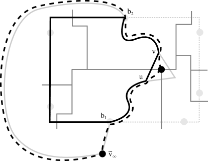
Figure 3: Example of a $2$-cycle separator of ${R}_{\Delta}({u})$ and its corresponding embedding into the actual graph.

We can now state the main lemma of this section.

Lemma 4.

Let $w$ be a vertex of $R$. Assume there exists a data structure that takes as input a the representation $\{b_{1},x,y,b_{2}\}$ of a 2-cycle separator $S$ of $\mbox{Vor}({R},{u})$ going through $v_{\infty}$ and answers in $t$ time queries of the following form: Is $w$ in the bounded closed subset of the plane with boundary $S$? Then there exists an algorithm running in time $O(t\log r)$ that returns a set of at most $6$ Voronoi cells of $\mbox{Vor}({R},{u})$ such that one of them contains $w$.

Proof.

The algorithm uses the recursive decomposition of ${R}_{\Delta}({u})$ described in this section. Note that the decomposition consists of 2-cycle separators going through $v_{\infty}$. Thus, using the above embedding, each of the 2-cycle of the decomposition corresponds to a separator consisting of an edge $(x,y)$ and the shortest paths $P_{R}(x,b_{1})$ and $P_{R}(y,b_{2})$ where $b_{1},b_{2}$ are boundary vertices of $R$. Additionally, $y$ belongs to the Voronoi cell of $b_{2}$ in $\mbox{Vor}({R},{u})$ and $x$ belongs to the Voronoi cell of $b_{1}$ in $\mbox{Vor}({R},{u})$. Therefore, $P_{R}(x,b_{1})$ and $P_{R}(y,b_{2})$ are vertex disjoint and so the data structure can be used to decide on which side of such a separator $w$ is.

The algorithm is the following: proceed recursively along the recursive decomposition of ${R}_{\Delta}({u})$ and for each $2$-cycle separator of the decomposition use the data structure to decide in $t$ time in which side of the 2-cycle $w$ is located and then recurse on this side. If $w$ belongs to both sides, i.e., if $w$ is on the $2$-cycle separator, recurse on an arbitrary side. The algorithm stops when there are at most $6$ faces of ${R}_{\Delta}({u})$ and then it returns the Voronoi cells of $\mbox{Vor}({R},{u})$ intersecting those $6$ faces.

Observe that the separators do not cross. Thus, when the algorithm obtains at a given recursive call that $w$ is in the interior (resp. exterior) of a 2-cycle $S$ and in the exterior (resp. interior) of the 2-cycle separator $S^{\prime}$ corresponding to the next recursive call, we can deduce that $w$ lies in the intersection of the interior of $S$ and the exterior of $S^{\prime}$ and hence deduce that it belongs to a Voronoi cell that lies in this area of the plane.

Note that by Lemma 2 the number of faces of ${R}_{\Delta}({u})$ in a piece decreases by a constant factor at each step. Thus, since the number of boundary vertices is $O(\sqrt{r})$, the procedure takes at most $O(t\log r)$ time.

Finally, observe that each face of ${R}_{\Delta}({u})$ that is adjacent to $v_{\infty}$ lies in a single Voronoi cell of $\mbox{Vor}({R},{u})$. Thus, since at the end of the recursion there are at most $6$ faces in the piece, they correspond to at most $6$ different Voronoi cells of $\mbox{Vor}({R},{u})$. Hence the algorithm returns at most $6$ different Voronoi cells of $\mbox{Vor}({R},{u})$.

∎

5 Preprocessing a Region

Given a query separator $S$ in a graph $R_{H}=R$ and given a query vertex $w$ in $R$, our data structure needs to determine in $O(1)$ time the side of $S$ that $w$ belongs to. In this section, we describe the preprocessing needed for this.

In the following, fix $R$ as well as an ordered pair $(u,v)$ of vertices of $R$ such that either $(u,v)$ or $(v,u)$ is an edge of $R$. The preprocessing described in the following is done over all such choices of $R$ and $(u,v)$ (and all holes $H$).

The vertices of $\delta R$ are on a simple cycle and we identify $\delta R$ with this cycle which we orient clockwise (ignoring the edge orientations of $R$). We let $b_{0},\ldots,b_{k}$ denote this clockwise ordering where $b_{k}=b_{0}$. It will be convenient to calculate indices modulo $k$ so that, e.g., $b_{k+1}=b_{1}$.

Given vertices $w$ and $w^{\prime}$ in $R$, let $P(w,w^{\prime})$ denote the shortest path in $R$ from $w$ to $w^{\prime}$. Given two vertices $b_{i},b_{j}\in\delta R$, we let $\delta(b_{i},b_{j})$ denote the subpath of cycle $\delta R$ consisting of the vertices from $b_{i}$ to $b_{j}$ in clockwise order, where $\delta(b_{i},b_{j})$ is the single vertex $b_{i}$ if $i=j$ and $\delta(b_{i},b_{j})=\delta R$ if $j=i+k$. We let $\Delta(w,b_{i},b_{j})$ denote the subgraph of $R$ contained in the closed and bounded region of the plane with boundary defined by $P(b_{i},w)$, $P(b_{j},w)$, and $\delta(b_{i},b_{j})$. We refer to $\Delta(w,b_{i},b_{j})$ as a wedge and call it a basic wedge if $b_{i}$ and $b_{j}$ are consecutive in the clockwise order, i.e., if $j=i+1\pmod{k}$. We need the following lemma.

Lemma 5.

Let $w$ be a given vertex of $R$. Then there is a data structure with $O(r)$ preprocessing time and size which answers in $O(1)$ time queries of the following form: given a vertex $x\in V(R)$ and two distinct vertices $b_{i_{1}},b_{i_{2}}\in\delta R$, does $x$ belong to $\Delta(w,b_{i_{1}},b_{i_{2}})$?

Proof.

Below we present a data structure with the bounds in the lemma which only answers restricted queries of the form “does $x$ belong to $\Delta(w,b_{0},b_{i})$?” for query vertices $x\in V(R)$ and $b_{i}\in\delta R$. In a completely symmetric manner, we obtain a data structure for restricted queries of the form “does $x$ belong to $\Delta(w,b_{i},b_{k})$?” for query vertices $x\in V(R)$ and $b_{i}\in\delta R$. We claim that this suffices to show the lemma. For consider a query consisting of $x\in V(R)$ and $b_{i},b_{j}\in\delta R$. If $b_{0}\in\delta(b_{i},b_{j})$ then $\Delta(w,b_{i},b_{j})=\Delta(w,b_{i},b_{k})\cup\Delta(w,b_{0},b_{j})$ and otherwise, $\delta(w,b_{i},b_{j})=\Delta(w,b_{0},b_{j})\cap\Delta(w,b_{i},b_{k})$. Hence, answering a general query can be done using two restricted queries and checking if $b_{0}\in\delta(b_{1},b_{2})$ can be done in constant time by comparing indices of the query vertices.

It remains to present the data structure for restricted queries of the form “does $x$ belong to $\Delta(w,b_{0},b_{i})$?”. In the preprocessing step, each $v\in V(R)$ is assigned the smallest index $i_{v}\in\{0,\ldots,k\}$ for which $v\in\Delta(w,b_{0},b_{i_{v}})$. Clearly, this requires only $O(r)$ space and below we show how to compute these indices in $O(r)$ time.

Consider a restricted query specified by a vertex $x$ of $R$ and a boundary vertex $b_{i}\in\delta R$ where $0\leq i\leq k$. Since $x\in\Delta(w,b_{0},b_{i})$ iff $i_{x}\leq i$, this query can clearly be answered in $O(1)$ time.

It remains to show how the indices $i_{v}$ can be computed in a total of $O(r)$ time. Let $R^{\prime}$ be $R$ with all its edge directions reversed. In $O(r)$ time, a SSSP tree $T^{\prime}$ from $w$ in $R^{\prime}$ is computed. Let $T$ be the tree in $R$ obtained from $T^{\prime}$ by reversing all its edge directions; note that all edges of $T$ are directed towards $w$ and for each $v\in V(R)$, the path from $v$ to $w$ in $T$ is a shortest path from $v$ to $w$ in $R$.

Next, $\Delta(w,b_{0},b_{0})=P(b_{0},w)$ is computed and for each vertex $v\in\Delta(w,b_{0},b_{0})$, set $i_{v}=0$. The rest of the preprocessing algorithm consists of iterations $i=1,\ldots,k$ where iteration $i$ assigns each vertex $v\in V(\Delta(w,b_{0},b_{i}))\setminus V(\Delta(w,b_{0},b_{i-1}))$ the index $i_{v}=i$. This correctly computes indices for all vertices of $R$. In the following, we describe how iteration $i$ is implemented.

First, the path $P(b_{i},w)$ is traversed in $T$ until a vertex $v_{i}$ is encountered which previously received an index. In other words, $v_{i}$ is the first vertex on $P(b_{i},w)$ belonging to $\Delta(w,b_{0},b_{i-1})$. Note that $v_{i}$ is well-defined since $w\in\Delta(w,b_{0},b_{i-1})$. Vertices that are in $V(P(b_{i},v_{i}))\setminus\{v_{i}\}$ or in a subtree of $T$ rooted in a vertex of $V(P(b_{i},v_{i}))\setminus\{v_{i}\}$ and extending to the right of this path are assigned the index value $i$. Furthermore, vertices belonging to a subtree of $T$ rooted in a vertex of $V(P(b_{i-1},v_{i}))\setminus\{v_{i}\}$ and extending to the left of this path are assigned the index value $i$, except those on $P(b_{i-1},v_{i})$ (as they belong to $\Delta(w,b_{0},b_{i-1})$).

Since $R$ is connected, it follows that the vertices assigned an index of $i$ are exactly those belonging to $V(\Delta(w,b_{0},b_{i}))\setminus V(\Delta(w,b_{0},b_{i-1}))$ and that the running time for making these assignments is $O(|V(\Delta(w,b_{0},b_{i}))\setminus V(\Delta(w,b_{0},b_{i-1}))|+|P(b_{i-1},v_{i})-v_{i}|+1)$. Over all $i$, total running time is $O(r)$; this follows by a telescoping sums argument and by observing that vertex sets $V(P(b_{i-1},v_{i}))\setminus\{v_{i}\}$ are pairwise disjoint. ∎

Given distinct vertices $b_{i_{1}},b_{i_{2}}\in\delta R$, if $P(b_{i_{1}},u)$ and $P(b_{i_{2}},v)$ do not cross (but may touch and then split), let $\Box(b_{i_{1}},b_{i_{2}},u,v)$ denote the subgraph of $R$ contained in the closed and bounded region of the plane with boundary defined by $P(b_{i_{1}},u)$, $P(b_{i_{2}},v)$, $\delta(b_{i_{1}},b_{i_{2}})$, and an edge of $R$ between vertex pair $(u,v)$. In order to simplify notation, we shall omit $u$ and $v$ and simply write $\Box(b_{i_{1}},b_{i_{2}})$.

It follows from planarity that there is at most one $b_{i}\in\delta R$ such that $(u,v)$ belongs to $E(\Delta(u,b_{i},b_{i+1}))\setminus E(P(b_{i+1},u))$ when ignoring edge orientations. If $b_{i}$ exists, we refer to it as $b_{uv}$; otherwise $b_{uv}$ denotes some dummy vertex not belonging to $R$.

The goal in this section is to determine whether a given query vertex belongs to a given query subgraph $\Box(b_{i_{1}},b_{i_{2}})$. The following lemma allows us to decompose this subgraph into three simpler parts as illustrated in Figure 4. We will show how to answer containment queries for each of these simple parts.

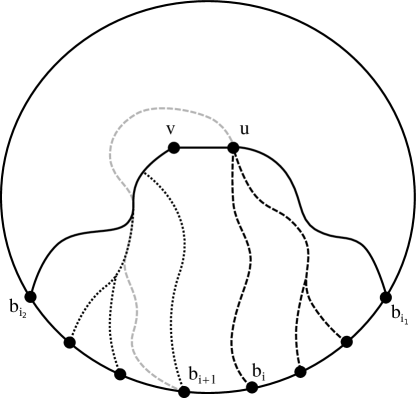
Figure 4: Example of decomposing the region into three parts using $b_{i}$: The dashed wedges represent shortest paths to $u$, the dotted edges represent shortest paths to $v$, and the dashed-dotted box $\Box(b_{i},b_{i+1})$.

Lemma 6.

Let $b_{i_{1}}$ and $b_{i_{2}}$ be distinct vertices of $\delta R$ and assume that $P(b_{i_{1}},u)$ and $P(b_{i_{2}},v)$ are vertex-disjoint. Then $\Box(b_{i_{1}},b_{i_{2}})=\Delta(u,b_{i_{1}},b_{i})\cup\Box(b_{i},b_{i+1})\cup\Delta(v,b_{i+1},b_{i_{2}})$ where $b_{i}=b_{uv}$ if $b_{uv}\in\delta(b_{i_{1}},b_{i_{2}-1})$ and $b_{i}=b_{i_{2}-1}$ otherwise.

Proof.

Figure 5 gives an illustration of the proof. We first show the following result: given a vertex $b_{j}\in\delta(b_{i_{1}+1},b_{i_{2}})$ such that $b_{uv}\notin\delta(b_{i_{1}},b_{j-1})$, $P(b_{j^{\prime}},u)$ is contained in $\Box(b_{i_{1}},b_{i_{2}})$ for each $b_{j^{\prime}}\in\delta(b_{i_{1}},b_{j})$. The proof is by induction on the number $i$ of edges in $\delta(b_{i_{1}},b_{j^{\prime}})$. The base case $i=0$ is trivial since then $b_{j^{\prime}}=b_{i_{1}}$ so assume that $i>0$ and that the claim holds for $i-1$. If $(v,u)$ is the last edge on $P(b_{j^{\prime}},u)$, the induction step follows from uniqueness of shortest paths. Otherwise, neither $(u,v)$ nor $(v,u)$ belong to $\Delta(u,b_{j^{\prime}-1},b_{j^{\prime}})$ (since $b_{j^{\prime}-1}\neq b_{uv}$). By the induction hypothesis, $P(b_{j^{\prime}-1},u)$ is contained in $\Box(b_{i_{1}},b_{i_{2}})$ and since $P(b_{j^{\prime}},u)$ cannot cross $P(b_{j^{\prime}-1},u)$, $P(b_{j^{\prime}},u)$ cannot cross $P(b_{i_{1}},u)$. Also, $P(b_{j^{\prime}},u)$ cannot cross $P(b_{i_{2}},v)$ since then either $(u,v)$ or $(v,u)$ would belong to $\Delta(u,b_{j^{\prime}-1},b_{j^{\prime}})$. Since $b_{j^{\prime}}\notin\{b_{i_{1}+1},b_{i_{2}-1}\}$, it follows that $P(b_{j^{\prime}},u)$ is contained in $\Box(b_{i_{1}},b_{i_{2}})$ which completes the proof by induction.

Next, assume that $b_{uv}\notin\delta(b_{i_{1}},b_{i_{2}-1})$ so that $b_{i}=b_{i_{2}-1}$. Note that $\Delta(v,b_{i+1},b_{i_{2}})=P(b_{i_{2}},v)$. Picking $b_{j}=b_{i_{2}}$ above implies that $\Delta(u,b_{i_{1}},b_{i})$ is contained in $\Box(b_{i_{1}},b_{i_{2}})$ and hence $\Box(b_{i_{1}},b_{i_{2}})=\Delta(u,b_{i_{1}},b_{i})\cup\Box(b_{i},b_{i+1})\cup\Delta(v,b_{i+1},b_{i_{2}})$.

Now consider the other case of the lemma where $b_{i}=b_{uv}\in\delta(b_{i_{1}},b_{i_{2}-1})$. Picking $b_{j}=b_{i}$ above, it follows that $\Delta(u,b_{i_{1}},b_{i})$ is contained in $\Box(b_{i_{1}},b_{i_{2}})$. It suffices to show that $P(b_{i+1},v)$ is contained in $\Box(b_{i_{1}},b_{i_{2}})$ since this will imply that $\Box(b_{i},b_{i+1})$ is well-defined and that $\Box(b_{i},b_{i+1})\cup\Delta(v,b_{i+1},b_{i_{2}})$ is contained in $\Box(b_{i_{1}},b_{i_{2}})$ and hence that $\Delta(u,b_{i_{1}},b_{i})\cup\Box(b_{i},b_{i+1})\cup\Delta(v,b_{i+1},b_{i_{2}})=\Box(b_{i_{1}},b_{i_{2}})$.

Assume for contradiction that $P(b_{i+1},v)$ is not contained in $\Box(b_{i_{1}},b_{i_{2}})$.

By uniqueness of shortest paths, $P(b_{i+1},u)$ does not cross $P(b_{i},u)$. Since $b_{i}=b_{uv}$, we have that when ignoring edge orientations, $(u,v)$ belongs to $E(\Delta(u,b_{i},b_{i+1}))\setminus E(P(b_{i+1},u))\subseteq E(\Delta(u,b_{i_{1}},b_{i+1}))\setminus E(P(b_{i+1},u))$. Hence $P(b_{i+1},u)$ is not contained in $\Box(b_{i_{1}},b_{i_{2}})$ so it crosses $P(b_{i_{2}},v)$. Let $x$ be a vertex on $P(b_{i+1},u)\cap P(b_{i_{2}},v)$ such that the successor of $x$ on $P(b{i+1},u)$ is not contained in $\Box(b_{i_{1}},b_{i_{2}})$. By our assumption above that $P(b_{i+1},v)$ is not contained in $\Box(b_{i_{1}},b_{i_{2}})$, there is a first vertex $y$ on $P(b_{i+1},v)$ such that its successor $y^{\prime}$ does not belong to $\Box(b_{i_{1}},b_{i_{2}})$. By uniqueness of shortest paths, $y$ cannot belong to $P(b_{i_{2}},v)$ so it must belong to $P(b_{i_{1}},u)$. This also implies that $y\neq x$ since $x\in P(b_{i_{2}},v)$ and $P(b_{i_{1}},u)$ and $P(b_{i_{2}},v)$ are vertex-disjoint. Since $P(y,v)$ is a subpath of $P(b_{i+1},v)$ and $y\neq x$, shortest path uniqueness implies that $P(y,v)$ and $P(b_{i+1},u)$ are vertex-disjoint.

Since $P(b_{i+1},y)$ is contained in $\Box(b_{i_{1}},b_{i_{2}})$, $v$ belongs to the subgraph of $\Delta(u,b_{i_{1}},b_{i+1})$ contained in the closed region of the plane bounded by $P(b_{i+1},y)$, $P(y,u)$, and $P(b_{i+1},u)$. Since $P(y,v)$ does not intersect $P(b_{i+1},u)$, $P(y^{\prime},v)$ thus intersects either $P(b_{i+1},y)$ or $P(y,u)$. However, it cannot intersect $P(b_{i+1},y)$ since then $P(b_{i+1},v)$ would be non-simple. By uniqueness of shortest paths, $P(y^{\prime},v)$ also cannot intersect $P(y,u)$ since $P(y^{\prime},v)$ is a subpath of $P(y,v)$ and $y^{\prime}\notin P(y,u)$. This gives the desired contradiction, concluding the proof. ∎

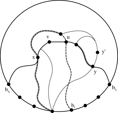
Figure 5: Illustration of the proof of Lemma 6. The figure shows how unique shortest paths imply a contradiction (highlighted with grey) if the path from $b_{i+1}$ to $v$ is not contained in $\Box(b_{i_{1}},b_{i_{2}})$.

Let $\mathcal{P}$ be a collection of subpaths such that for each path $\delta(b_{i_{1}},b_{i_{2}})$ in $\mathcal{P}$, $b_{uv}\notin\delta(b_{i_{1}},\ldots,b_{i_{2}-1})$ and $b_{vu}\notin\delta(b_{i_{1}+1},\ldots,b_{i_{2}-1})$. We may choose the paths such that $|\mathcal{P}|=O(1)$ and such that all edges of $\delta R$ except $(b_{uv},b_{vu})$ (if it exists) belongs to a path of $\mathcal{P}$. It is easy to see that this is possible by considering a greedy algorithm which in each step picks a maximum-length path which is edge-disjoint from previously picked paths and which satisfies the two stated requirements.

The next lemma allows us to obtain a compact data structure to answer queries of the form “does face $f$ belong to $\Box(b_{i},b_{i+1})$” for given query face $f$ and query index $i$.

Lemma 7.

Let $P=\delta(b_{i_{1}},b_{i_{2}})\in\mathcal{P}$ be given. Then

1. an index $j(P)$ exists with $i_{1}\leq j(P)\leq i_{2}$ such that $\Box(b_{i},b_{i+1})$ is undefined for $i_{1}\leq i<j(P)$ and well-defined for $j(P)\leq i<i_{2}$,

2. for each face $f\neq\delta R$ of $R$, there is at most one index $j_{f}(P)$ with $j(P)\leq j_{f}(P)\leq i_{2}-2$ such that $f\subseteq\Box(b_{j_{f}(P)},b_{j_{f}(P)+1})$ and $f\nsubseteq\Box(b_{j_{f}(P)+1},b_{j_{f}(P)+2})$, and

3. for each face $f\neq\delta R$ of $R$, there is at most one index $j_{f}^{\prime}(P)$ with $j(P)\leq j_{f}^{\prime}(P)\leq i_{2}-2$ such that $f\nsubseteq\Box(b_{j_{f}^{\prime}(P)},b_{j_{f}^{\prime}(P)+1})$ and $f\subseteq\Box(b_{j_{f}^{\prime}(P)+1},b_{j_{f}^{\prime}(P)+2})$.

Furthermore, there is an algorithm which computes the index $j(P)$ and for each face $f\neq\delta R$ of $R$ the indices $j_{f}(P)$ and $j_{f}^{\prime}(P)$ if they exist. The total running time of this algorithm is $O(r\log r)$ and its space requirement is $O(r)$.

Proof.

Let path $P=\delta(b_{i_{1}},b_{i_{2}})\in\mathcal{P}$ and face $f\neq\delta R$ of $R$ be given. To simplify notation in the proof, we shall omit reference to $P$ and write, e.g., $j$ instead of $j(P)$.

Let $j$ be the smallest index such that $\Box(b_{j},b_{j+1})$ is well-defined; if $j$ does not exist, pick instead $j=i_{2}$. We will show that $j$ satisfies the first part of the lemma. This is clear if $j=i_{2}$ so assume therefore in the following that $j<i_{2}$.

We prove by induction on $i$ that $\Box(b_{i},b_{i+1})$ is well-defined for $j\leq i<i_{2}$. By definition of $j$, this holds when $i=j$. Now, consider a well-defined subgraph $\Box(b_{i},b_{i+1})$ where $j\leq i\leq i_{2}-2$. We need to show that $\Box(b_{i+1},b_{i+2})$ is well-defined. Since $b_{i}\neq b_{uv}$, $P(b_{i+1},u)$ is contained in $\Box(b_{i},b_{i+1})$ and since $b_{i+1}\neq b_{vu}$, $P(b_{i+2},v)$ is contained in the closed region of the plane bounded by the boundary of $\Box(b_{i},b_{i+1})$ and not containing $\Box(b_{i},b_{i+1})$. In particular, $\Box(b_{i+1},b_{i+2})$ is well-defined. This shows the first part of the lemma.

Next, we show that $j$ can be computed in $O(r\log r)$ time. Checking that $\Box(b_{i},b_{i+1})$ is well-defined (i.e., that paths $P(b_{i},u)$ and $P(b_{i+1},v)$ do not cross) for a given index $i$ can be done in $O(r)$ time. Because of the first part of the lemma, a binary search algorithm can be applied to identify $j$ in $O(\log r)$ steps where each step checks if $\Box(b_{i},b_{i+1})$ is well-defined for some index $i$. This gives a total running time of $O(r\log r)$, as desired. Space is clearly $O(r)$.

To show the second part of the lemma, assume that there is an index $j_{f}$ with $i_{1}\leq j_{f}\leq i_{2}-2$ such that $f\subseteq\Box(b_{j_{f}},b_{j_{f}+1})$ and $f\nsubseteq\Box(b_{j_{f}+1},b_{j_{f}+2})$. It follows from the observations in the inductive step above that $\Delta(u,b_{j_{f}},b_{j_{f}+1})$ contains exactly the faces of $R$ contained in $\Box(b_{j_{f}},b_{j_{f}+1})$ and not in $\Box(b_{j_{f}+1},b_{j_{f}+2})$ which implies that $f\subseteq\Delta(u,b_{j_{w}},b_{j_{w}+1})$. Since no face of $R$ belongs to more than one graph of the form $\Delta(u,b_{i},b_{i+1})$, $j_{f}$ must be unique, showing the second part of the lemma.

Next, we give an $O(r)$ time and space algorithm that computes indices $j_{f}$. Let $T$ be constructed as in the proof of Lemma 5. Initially, vertices of $P(b_{i_{2}-1},u)$ are marked and all other vertices of $R$ are unmarked. The remaining part of the algorithm consists of iterations $i_{2}-2,\ldots,j$ in that order. In iteration $i$, $P(b_{i},u)$ is traversed until a marked vertex $v_{i}$ is visited and then the vertices of $P(b_{i},v_{i})$ are marked. The faces of $R$ contained in the bounded region of the plane defined by $P(b_{i},v_{i})$, $P(b_{i+1},v_{i})$, and $\delta(b_{i},b_{i+1})$ are exactly those that should be given an index value of $i$. The algorithm performs this task by traversing each subtree of $T$ emanating to the right of $P(b_{i},v_{i})$ and each subtree of $T$ emanating to the left of $P(b_{i+1},v_{i})$; for each vertex visited, the algorithm assigns the index value $i$ to its incident faces.

We now show that the algorithm for computing indices $j_{f}$ has $O(r)$ running time. Using the same arguments as in the proof of Lemma 5, the total time to traverse and mark paths $P(b_{i},v_{i})$ is $O(r)$. The total time to assign indices to faces is $O(r)$; this follows by observing that the time spent on assigning indices to faces incident to a vertex of $T$ is bounded by its degree and this vertex is not visited in other iterations.

The third part of the lemma follows with essentially the same proof as for the second part. ∎

We can now combine the results of this section to obtain the data structure described in the following lemma.

Lemma 8.

Let $(u,v)$ be a vertex pair connected by an edge in $R$. Then there is a data structure with $O(r\log r)$ preprocessing time and $O(r)$ space which answers in $O(1)$ time queries of the following form: given a vertex $w\in R$ and two distinct vertices $b_{i},b_{j}\in\delta R$ such that $P(b_{i},u)$ and $P(b_{j},v)$ are vertex-disjoint, does $w$ belong to $\Box(b_{i},b_{j},u,v)$?

Proof.

We present a data structure $\mathcal{D}(u,v)$ satisfying the lemma. First we focus on the preprocessing. Boundary vertices $b_{uv}$ and $b_{vu}$ and set $\mathcal{P}$ as defined above are precomputed and stored. Vertices of $\delta R$ are labeled with indices $b_{0},\ldots,b_{|V(\delta R)|-1}$ according to a clockwise walk of $\delta R$. Each path of the form $\delta(b_{i_{1}},b_{i_{2}})$ (including each path in $\mathcal{P}$) is represented by the ordered index pair $(i_{1},i_{2})$. Checking if a given boundary vertex belongs to such a given path can then be done in $O(1)$ time.

Next, two instances of the data structure in Lemma 5 are set up, one for $u$ denoted $\mathcal{D}_{u}$, and one for $v$ denoted $\mathcal{D}_{v}$. Then the following is done for each path $P=\delta(b_{i_{1}},b_{i_{2}})\in\mathcal{P}$. First, the algorithm in Lemma 7 is applied. Then if $\Box(b_{j(P)},b_{j(P)+1},u,v)$ is well-defined, its set of faces $F_{j(P)}$ is computed and stored; otherwise, $F_{j(P)}=\emptyset$. Similarly, if $\Box(b_{i_{2}-1},b_{i_{2}},u,v)$ is well-defined, its set of faces $F_{i_{2}-1}$ is computed and stored, and otherwise $F_{i_{2}-1}=\emptyset$. If $(b_{uv},b_{vu})\in\delta R$, $\mathcal{D}(u,v)$ computes and stores the set $F_{uv}$ of faces of $R$ contained in $\Box(b_{uv},b_{vu},u,v)$. This completes the description of the preprocessing for $\mathcal{D}(u,v)$. It is clear that preprocessing time is $O(r\log r)$ and that space is $O(r)$.

Now, consider a query specified by a vertex $w\in R$ and two distinct vertices $b_{i_{1}},b_{i_{2}}\in\delta R$ such that $P(b_{i_{1}},u)$ and $P(b_{i_{2}},v)$ are pairwise vertex-disjoint. First, $\mathcal{D}(u,v)$ identifies a boundary vertex $b_{i}$ such that $\Box(b_{i_{1}},b_{i_{2}},u,v)=\Delta(u,b_{i_{1}},b_{i})\cup\Box(b_{i},b_{i+1})\cup\Delta(v,b_{i+1},b_{i_{2}})$; this is possible by Lemma 6. Then $\mathcal{D}_{u}$ and $\mathcal{D}_{v}$ are queried to determine if $w\in\Delta(u,b_{i_{1}},b_{i})\cup\Delta(v,b_{i+1},b_{i_{2}})$; if this is the case then $w\in\Box(b_{i_{1}},b_{i_{2}},u,v)$ and $\mathcal{D}(u,v)$ answers “yes”. Otherwise, $\mathcal{D}(u,v)$ identifies an arbitrary face $f\neq\delta R$ of $R$ incident to $w$. At this point, the only way that $w$ can belong to $\Box(b_{i_{1}},b_{i_{2}},u,v)$ is if $w$ belongs to the interior of $\Box(b_{i},b_{i+1},u,v)$ which happens iff $f$ is contained in $\Box(b_{i},b_{i+1},u,v)$. If $(b_{i},b_{i+1})=(b_{uv},b_{vu})$, $\mathcal{D}(u,v)$ checks if $f\in F_{uv}$ and if so outputs “yes”. Otherwise, there exists a path $P\in\mathcal{P}$ containing $(b_{i},b_{i+1})$ and $\mathcal{D}(u,v)$ identifies this path. It follows from Lemma 7 and from the definition of $\mathcal{P}$ that $f$ is contained in $\Box(b_{i},b_{i+1},u,v)$ iff at least one of the following conditions hold:

1. $j_{f}(P)$ and $j_{f}^{\prime}(P)$ are well-defined and $j_{f}^{\prime}(P)<i\leq j_{f}(P)$.

2. $f\in F_{i_{2}-1}$, $j_{f}^{\prime}(P)$ is well-defined, and $i>j_{f}^{\prime}(P)$,

3. $f\in F_{j(P)}$, $j_{f}(P)$ is well-defined, and $i\leq j_{f}(P)$,

4. $f\in F_{j(P)}$ and $j_{f}(P)$ is undefined,

Data structure $\mathcal{D}(u,v)$ checks if any one these conditions hold and if so outputs “yes”; otherwise it outputs “no”. Two of the cases are illustrated in Figure 6.

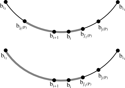
Figure 6: Illustration of how to determine if the face $f$ belongs to $\Box(b_{i},b_{i+1},u,v)$. The illustration includes cases 1 and 4 in the proof of Lemma 8. The large gray subpath indicates the part, where $f$ is contained in each box defined by consecutive boundary nodes.

It remains to show that $\mathcal{D}(u,v)$ has query time $O(1)$. By Lemma 6, identifying $b_{k}$ can be done in $O(1)$ time. Querying $\mathcal{D}_{u}$ and $\mathcal{D}_{v}$ takes $O(1)$ time by Lemma 5. Checking whether $f\in F_{uv}$ can clearly be done in $O(1)$ time since this set of faces is stored explicitly. With our representation of paths by the indices of their endpoints, identifying $P$ takes $O(1)$ time. Finally, since sets $F_{j(P)}$ and $F_{j(P)}$ are explicitly stored, the four conditions above can be checked in $O(1)$ time. ∎

6 The Distance Oracle

In this section we give a detailed presentation of both our algorithm for answering distance queries and our distance oracle data structure.

Combining Lemmas 9, 10 and 11 with $r=n^{2/3}$ directly implies Theorem 1.

6.1 The Data Structure

We present the algorithm for building our data structure.

Preprocessing $G$

1. Compute an $r$-division $\mathcal{R}$ of $G$. Let $\delta$ be the set of all boundary vertices.

2. Store for each internal vertex the region to which it belongs.

3. Compute and store the distances from each vertex to each boundary vertex.

4. For each region $R\in\mathcal{R}$, compute and store the distances between any pair of internal vertices of $R$.

5. For each region $R$, for each vertex $u\notin R$, for each hole $H$, compute $\text{Vor}_{H}(R,u)$ and store a separator decomposition as described in Section 4.

6. For each region $R$, for each edge $(x,y)\in R$, for each hole $H$, compute and store the data structure described in Section 5.

Lemma 9.

The total size of the data structure computed by Preprocessing is $O(n^{2}/\sqrt{r}+n\cdot r)$.

Proof.

Recall that by definition of the $r$-division, there are $O(n/\sqrt{r})$ boundary vertices and $O(n/r)$ regions. Thus, the number of distances stored at step 3 of the algorithm is at most $O(n^{2}/\sqrt{r})$.

For a given region, storing the pairwise distances between all its internal vertices takes $O(r^{2})$ space. Since there are $O(n/r)$ regions in total, Step 4 takes memory $O(n\cdot r)$.

We now bound the space taken by Step 5. There are $n/r$ choices for $R$ and $n$ choices for $u$. By Lemma 3, each decomposition can be stored using $O(\sqrt{r})$ space. Thus, this step takes $O(n^{2}/\sqrt{r})$ total space.

We finally bound the space taken by Step 6. There $n/r$ choices for $R$ and $r$ choices for an edge $(x,y)$.By Lemma 8, for a given edge $(x,y)$, the data structure takes $O(r)$ space. Hence, the total space taken by this step is $O(n\cdot r)$ and the lemma follows. ∎

Theorem 3.

The execution of Preprocessing takes $O(n^{2})$ time and $O(n\cdot r+n^{2}/\sqrt{r})$ space.

Proof.

We analyze the procedure step by step. Computing an $r$-division with $O(1)$ holes can be done in linear time and space using the algorithm of Klein et al., see [23].

We now analyze Step 3. There are $O(n/\sqrt{r})$ boundary vertices. Computing single-source shortest paths can be done in linear time using the algorithm of Henzinger et al. [16]. Hence, Step 3 takes at most $O(n^{2}/\sqrt{r})$ time and space.

Step 4 takes $O(n\cdot r)$ time and space using the following algorithm. The algorithm proceed region by region and hole by hole. For a given region and hole, the algorithm adds an edge between each pair of boundary vertices that are on the hole of length equal to the distance between these vertices in the whole graph. Note that this is already in memory and was computed at Step 3. Now, for each vertex of the region, the algorithm runs a shortest path algorithm. Since there are $O(\sqrt{r})$ boundary vertices, the number of edges added is $O(r)$. Thus, the algorithm is run on a graph that has at most $O(r)$ edges and vertices. The algorithm spends at most $O(r)$ time per vertex of the region. Since there are $O(n/r)$ regions and $O(r)$ vertices per region, both the running time and the space are $O(n\cdot r)$.

Step 5 takes $O(n^{2})$ using the following algorithm. The algorithm proceeds vertex by vertex, region by region, hole by hole. For a given vertex $u$, a given region $R$, and a given hole $H$ the algorithm computes $\text{Vor}_{H}(R,u)$. This can be done by adding a “dummy” vertex reprensenting $u$ and connecting it to each boundary vertex $x$ of the hole by an edge of length $\text{dist}(u,x)$. Thus, this takes time $O(r)$ using the single-source shortest path algorithm of Henzinger et al [16]. Furthermore, by Lemma 3 and Corollary 1, computing the separator decomposition of Section 4 given $\text{Vor}_{H}(R,u)$ takes $\tilde{O}(\sqrt{r})$ time and $O(\sqrt{r})$ space. Thus, over all vertices, regions and holes, this step takes $O(n^{2})$ time and $O(n^{2}/\sqrt{r})$ memory.

Finally, we show that Step 6 takes $\tilde{O}(n\cdot r)$ time and $O(n\cdot r)$ space. The algorithm proceeds region by region, hole by hole, and edge by edge. By Lemma 8, for a given edge of the region, computing the data structure of Section 5 takes $O(r\cdot\log r)$ time and space. Since the total number of region is $O(n/r)$ and the total number of edges per region is $O(r)$, the proof is complete. ∎

Corollary 2.

There exists a distance oracle with total space $O(n^{11/6})$ and expected preprocessing time $O(n^{11/6})$.

Proof.

We apply Procedure Preprocessing with $r=n^{1/3}$. By Lemma 9, the total size of the data structure output is $O(n^{11/6})$.

We now analyse the total preprocessing time. For Steps 3, 4, and 6, we mimicate the analysis of the proof of Theorem 3 and obtain a total preprocessing time of $O(n\cdot r+n^{2}/\sqrt{r})$.

We now explain how to speed-up Step 5. We show that Step 5 can be done in time $O(n\cdot r^{5/2})$ using Cabello’s data structure [5] for computing weighted Voronoi diagrams of a given region.

More formally, Cabello introduces a data structure that allows to compute weighted Voronoi diagrams of a given region in expected time $\tilde{O}(\sqrt{r})$. This data structure has preprocessing time $O(r^{7/2})$. Hence the total preprocessing time for computing the data structure for all the regions is $\tilde{O}(n\cdot r^{5/2})$.

Then, for each vertex $u$, each region $R$, each hole $H$, the algorithm

1. uses the data structure to compute the weighted Voronoi diagram $\text{Vor}_{H}(R,u)$ in expected time $\tilde{O}(\sqrt{r})$ and

2. computes the separator decomposition of Section 4 in time $\tilde{O}(\sqrt{r})$ (by Lemma 3 and Corollary 1).

This results in an expected preprocessing time of $O(n\cdot r^{5/2}+n^{2}/\sqrt{r})$. Choosing $r=n^{1/3}$ yields a bound of $O(n^{11/6})$. ∎

6.2 Algorithm for Distance Queries

This section is devoted to the presentation of our algorithms for answering distance queries between pairs of vertices.

We show that any distance query between two vertices $u$, $v$ can be performed in $O(\log r)$ time. In the following, let $u,v$ be two vertices of the graph. The algorithm is the following.

Distance Query $u,v$

1. If $u,v$ belong to the same region or if either $u$ or $v$ is a boundary vertex, the query can be answered in $O(1)$ time since the distances between vertices of the same region and between boundary vertices and the other vertices of the graph are stored explicitly.

2. If $u$ and $v$ are internal vertices that belong to two different regions we proceed as follows. Let $R$ be the region containing $v$ and $\delta R$ be the set of boundary vertices of region $R$. The boundary vertices are partitioned into holes $\mathcal{H}=\{H_{0},\ldots,H_{k}\}$, such that $\bigcup_{H\in\mathcal{H}}H=\delta R$. For each $H\in\mathcal{H}$, we apply the following procedure. Let $\mathcal{V}$ be the weighted Voronoi diagram where the sites are the vertices of $H$ and the weight of $x\in H$ is the distance from $u$ to $x$.

   We now aim at determining to which cell of $\mathcal{V}$, $v$ belongs. We use the binary search procedure of Lemma 4 on the decomposition of $R$ induced by the separators of the weighted Voronoi diagram. More precisely, we use the algorithm described in Section 4, Lemma 4, and the query algorithm described in Section 5, Lemma 8 to identify a set of at most six Voronoi cells so that one of them contains $v$. This induces a set of at most six boundary vertices $X=\{x_{0},\ldots,x_{k}\}$ that represent the centers of the cells.

   Finally, we have the distances from both $u$ and $v$ to all the boundary vertices in $X$. Let $v(H)=\min_{x\in X}\text{dist}(u,x)+\text{dist}(x,v)$. The algorithm returns $\min_{H\in\mathcal{H}}v(H)$.

Lemma 10 (Running time).

The Distance Query takes $O(\log r)$ time.

Proof.

Consider a distance query from a vertex $u$ to a vertex $v$ and assume that those vertices are internal vertices of two different regions as otherwise the query takes $O(1)$ time. Observe that we can determine in $O(1)$ time to which region $v$ belongs. Fix a hole $H$. Let $\mathcal{V}$ be the weighted Voronoi diagram where the sites are the vertices of $H$ and the weight of $x\in\delta R$ is the distance from $u$ to $x$. We consider the decomposition of the region of $v$ of $\mbox{Vor}({R},{u})$.

Lemma 8 shows that the query time for the data structure defined in Section 5 is $t=O(1)$. Applying Lemma 4 with $t=O(1)$ implies that the total time to determine in which Voronoi cell $v$ belongs is at most $O(\log r)$.

Finally, computing $\min_{x\in X}\text{dist}(u,x)+\text{dist}(x,v)$ takes $O(1)$ time. By definition of the $r$-division there are $O(1)$ holes.

Therefore, we conclude that the running time of the Distance Query algorithm is $O(\log r)$. ∎

We now prove that the algorithm indeed returns the correct distance between $u$ and $v$.

Lemma 11 (Correctness).

The Distance Query on input $u,v$ returns the length of the shortest path between vertices $u$ and $v$ in the graph.

Proof.

We remark that the distance from any vertex to a boundary vertex is stored explicitly and thus correct. Hence, we consider the case where $u$ and $v$ are internal vertices of different regions. Let $P$ be the shortest path from $u$ to $v$ in $G$. Let $x\in P$ be the last boundary vertex of $R$ on the path from $u$ to $v$ and let $H_{x}$ be the hole containing $x$. Let $\mathcal{V}$ be the weighted Voronoi diagram where the sites are the boundary vertices of $H_{x}$ and the weight of $y\in H_{x}$ is the distance from $u$ to $y$.

We need to argue that the data structure of Section 5, Lemma 8 satisfies the conditions of Lemma 4. Observe that the separators defined in Section 4 consist of two shortest paths $P_{R}(b_{1},x)$ and $P_{R}(b_{2},y)$ where $b_{1},b_{2}\in\delta R$ and $(y,z)$is an edge of $R$. Hence, the set of vertices of the subgraph $\Box(b_{1},b_{2},y,z)$ correspond to the set of all the vertices that are one of the two sides of the separator. Thus, by Lemma 8 the data structure described in Section 5 satisfies the condition of Lemma 4, with query time $t=O(1)$.

We argue that $v$ belongs to the Voronoi cell of $x$. Assume towards contradiction that $v$ is in the Voronoi cell of $y\neq x$, we would have $\text{dist}(y,v)+w(y)\leq\text{dist}(x,v)+w(x)$, where $w$ is the weight function associated with the Voronoi diagram. Thus, this implies that $\text{dist}(y,v)+\text{dist}(y,u)\leq\text{dist}(x,v)+\text{dist}(x,u)$. Therefore, there exists a shortest path from $u$ to $v$ that goes through $y$. Now observe that if $v$ belongs to the Voronoi cell of $y$, the shortest path from $v$ to $y$ does not go through $x$. Hence, assuming unique shortest paths between pairs of vertices, we conclude that the last boundary vertex on the path from $u$ to $v$ is $y$ and not $x$, a contradiction. Thus, $v$ belongs to the Voronoi cell of $x$.

Combining with Lemma 8, it follows that the Voronoi cell of $x$ is in the set of Voronoi cells $X$ obtained at the end of the recursive procedure. Observe that for any $x^{\prime}\in X$ there exists a path (possibly with repetition of vertices) of length $\text{dist}(x^{\prime},u)+\text{dist}(x^{\prime},v)$. Therefore, since we assume unique shortest paths between pairs of vertices, we conclude that $\text{dist}(u,v)=\text{dist}(x,u)+\text{dist}(x,v)=\min_{x^{\prime}\in X}\text{dist}(x^{\prime},v)+\text{dist}(x^{\prime},u)=v(H_{x})=\min_{H}v(H)$. ∎

7 Trade-off

We now prove Theorem 2. We first consider the case with $P=O(n^{2})$ and then extend it to the case with efficient preprocessing time.

Let $r_{1}\leq r_{2}$ be positive integers to be defined later. The case $r_{1}\leq r_{2}$ will correspond exactly to $S\geq n\sqrt{n}$. The data structure works as follows.

1. We compute an $r_{1}$-division and an $r_{2}$-division of $G$ named $\mathcal{R}_{1}$ and $\mathcal{R}_{2}$ respectively. Let $\delta_{1}$ respectively $\delta_{2}$ denote all the boundary vertices of $\mathcal{R}_{1}$ resp. $\mathcal{R}_{2}$.

2. For each region $R$ of $\mathcal{R}_{1}$ and $\mathcal{R}_{2}$, compute and store the pairwise distances of the nodes of $R$.

3. For each $u\in\delta_{1}$ and $v\in\delta_{2}$, compute and store the distance between $u$ and $v$ in $G$.

4. For each $u\in\delta_{1}$, region $R\in\mathcal{R}_{2}$ and hole $H\in R$, compute $\text{Vor}_{H}(R,u)$ and store a separator decomposition as described in Section 4.

5. For each Region $R\in\mathcal{R}_{2}$, for each edge $(x,y)\in R$, for each hole $H$, compute and store the data structure described in Section 5.

We start by bounding the space.

Lemma 12.

The total size of the data structure described above is

$$O\!\left(nr_{2}+\frac{n^{2}}{\sqrt{r_{1}r_{2}}}\right)\ .$$

Proof.

Consider the steps above. By definition of $\mathcal{R}_{1}$ and $\mathcal{R}_{2}$ step 2 uses $O(nr_{2})$ space (since we assumed $r_{1}\leq r_{2}$) and step 4 uses $\frac{n}{\sqrt{r_{1}}}\cdot\frac{n}{\sqrt{r_{2}}}$ space. By Lemma 3 step 5 takes $O(n/\sqrt{r_{2}})$ for each node of $\delta_{1}$ giving $O(n^{2}/\sqrt{r_{1}r_{2}})$ in total. By Lemma 8 the total space of step 6 is $O(nr_{2})$. ∎

Now consider a query pair $u,v$. If $u$ and $v$ belong to the same region in $\mathcal{R}_{1}$ or $\mathcal{R}_{2}$ we return the stored distance. Otherwise we iterate over each boundary node $w$ in the region of $u$ in $\mathcal{R}_{1}$. For each such boundary node we compute the distance to $v$ using the data structures of steps 5 and 6 above similar to the query algorithm from Section 6.2. This is possible since we have stored the distances between all the needed boundary nodes in step 4. The minimum distance returned over all such $w$ is the answer to the query.

From the description above it is clear that we get a query time of $O(\sqrt{r_{1}}\log(r_{2}))$. The correctness follows immediately from the discussion in the proof of Theorem 1. What is left now is to balance the space to obtain Theorem 2. The expression of Lemma 12 is balanced when

$$r_{2}=\frac{n^{2/3}}{r_{1}^{1/3}}\ .$$

Now, since we assumed that $S\geq n\sqrt{n}$ we can focus on the case when $r_{2}\geq\sqrt{n}$ and thus we get $r_{1}\leq r_{2}$ as we required. Plugging into the definition of $Q$ we get exactly

$$Q=O(\sqrt{r_{1}}\log n)=\frac{n^{5/2}}{S^{3/2}}\log n\ ,$$

which gives us Theorem 2.

For pre-processing time, we consider two cases similar to Theorem 3 and Corollary 2. It follows directly from the discussion above and Theorem 3 that the preprocessing can be performed in $O(n^{2})$. We may, however, also consider pre-processing time as a parameter similar to space and query time. This gives a 3-way trade-off. In Corollary 2 we showed how to lower pre-processing time by increasing the space. Here we discuss the case of lowering pre-processing time further by increasing the query time. It follows from the discussion above and Corollary 2 that we can perform pre-processing of the above structure in $O(nr_{1}+nr_{2}^{5/2}+n^{2}/\sqrt{r_{1}r_{2}})$ time and get the same space bound. If we assume that $r_{1}\leq r_{2}^{5/2}$ we get a data structure with query time $Q=O(\sqrt{r_{1}}\log n)$ and space and pre-processing time $S=O(nr_{2}^{5/2}+n^{2}/\sqrt{r_{1}r_{2}})$. Up to logarithimic and constant factors, this gives us $Q=n^{11/5}/S^{6/5}$. For any $S\geq n^{16/11}$ this satisfies the requirement that $r_{1}\leq r_{2}^{5/2}$. As an example, we get a data structure with space and pre-processing time $O(n^{16/11})$ and a query time of $O(n^{5/11}\log n)$.

References

- [1] The TSPLIB. http://comopt.ifi.uni-heidelberg.de/software/TSPLIB95/. Accessed: 2010-09-30.
- [2] Amir Abboud and Søren Dahlgaard. Popular conjectures as a barrier for dynamic planar graph algorithms. In Proc. 57th IEEE Symposium on Foundations of Computer Science (FOCS), pages 477–486, 2016.
- [3] Srinivasa Rao Arikati, Danny Z. Chen, L. Paul Chew, Gautam Das, Michiel H. M. Smid, and Christos D. Zaroliagis. Planar spanners and approximate shortest path queries among obstacles in the plane. In Proc. 4th European Symposium on Algorithms (ESA), pages 514–528, 1996.
- [4] Sergio Cabello. Many distances in planar graphs. Algorithmica, 62(1-2):361–381, 2012. See also SODA’06.
- [5] Sergio Cabello. Subquadratic algorithms for the diameter and the sum of pairwise distances in planar graphs. In Proc. 28th ACM/SIAM Symposium on Discrete Algorithms (SODA), pages 2143–2152, 2017.
- [6] Shiri Chechik. Approximate distance oracles with constant query time. In Proc. 46th ACM Symposium on Theory of Computing (STOC), pages 654–663, 2014.
- [7] Shiri Chechik. Approximate distance oracles with improved bounds. In Proc. 47th ACM Symposium on Theory of Computing (STOC), pages 1–10, 2015.
- [8] Danny Z. Chen and Jinhui Xu. Shortest path queries in planar graphs. In Proc. 22nd ACM Symposium on Theory of Computing (STOC), pages 469–478, 2000.
- [9] Vincent Cohen-Addad, Søren Dahlgaard, and Christian Wulff-Nilsen. Fast and compact exact distance oracle for planar graphs. CoRR, abs/1702.03259, 2017.
- [10] Hristo Djidjev. On-line algorithms for shortest path problems on planar digraphs. In Graph-Theoretic Concepts in Computer Science, 22nd International Workshop, WG ’96, Cadenabbia (Como), Italy, June 12-14, 1996, Proceedings, pages 151–165, 1996.
- [11] Paul Erdős. Extremal problems in graph theory. In IN “THEORY OF GRAPHS AND ITS APPLICATIONS,” PROC. SYMPOS. SMOLENICE. Citeseer, 1964.
- [12] Jittat Fakcharoenphol and Satish Rao. Planar graphs, negative weight edges, shortest paths, and near linear time. Journal of Computer and System Sciences, 72(5):868–889, 2006. See also FOCS’01.
- [13] Greg N. Frederickson. Fast algorithms for shortest paths in planar graphs, with applications. SIAM Journal on Computing, 16(6):1004–1022, 1987.
- [14] Pawel Gawrychowski and Adam Karczmarz. Improved bounds for shortest paths in dense distance graphs. CoRR, abs/1602.07013, 2016.
- [15] Paweł Gawrychowski, Haim Kaplan, Shay Mozes, Micha Sharir, and Oren Weimann. Voronoi diagrams on planar graphs, and computing the diameter in deterministic o (n5/3) time, 2017. arXiv preprint.
- [16] Monika R Henzinger, Philip Klein, Satish Rao, and Sairam Subramanian. Faster shortest-path algorithms for planar graphs. Journal of Computer and System Sciences, 55(1):3–23, 1997.
- [17] Giuseppe F Italiano, Yahav Nussbaum, Piotr Sankowski, and Christian Wulff-Nilsen. Improved algorithms for min cut and max flow in undirected planar graphs. In Proc. 43rd ACM Symposium on Theory of Computing (STOC), pages 313–322, 2011.
- [18] Haim Kaplan, Shay Mozes, Yahav Nussbaum, and Micha Sharir. Submatrix maximum queries in monge matrices and monge partial matrices, and their applications. In Proc. 23rd ACM/SIAM Symposium on Discrete Algorithms (SODA), pages 338–355, 2012.
- [19] Ken-ichi Kawarabayashi, Philip N Klein, and Christian Sommer. Linear-space approximate distance oracles for planar, bounded-genus and minor-free graphs. In International Colloquium on Automata, Languages, and Programming, pages 135–146. Springer, 2011.
- [20] Ken-ichi Kawarabayashi, Christian Sommer, and Mikkel Thorup. More compact oracles for approximate distances in undirected planar graphs. In Proceedings of the Twenty-Fourth Annual ACM-SIAM Symposium on Discrete Algorithms, pages 550–563. SIAM, 2013.
- [21] Philip N. Klein. Preprocessing an undirected planar network to enable fast approximate distance queries. In Proc. 13th ACM/SIAM Symposium on Discrete Algorithms (SODA), pages 820–827, 2002.
- [22] Philip N Klein. Multiple-source shortest paths in planar graphs. In Proc. 16th ACM/SIAM Symposium on Discrete Algorithms (SODA), volume 5, pages 146–155, 2005.
- [23] Philip N Klein, Shay Mozes, and Christian Sommer. Structured recursive separator decompositions for planar graphs in linear time. In Proc. 45th ACM Symposium on Theory of Computing (STOC), pages 505–514. ACM, 2013.
- [24] Rolf Klein. Concrete and Abstract Voronoi Diagrams, volume 400 of Lecture Notes in Computer Science. Springer, 1989.
- [25] Rolf Klein, Elmar Langetepe, and Zahra Nilforoushan. Abstract voronoi diagrams revisited. Comput. Geom., 42(9):885–902, 2009.
- [26] Shay Mozes and Christian Sommer. Exact distance oracles for planar graphs. In Proc. 23rd ACM/SIAM Symposium on Discrete Algorithms (SODA), pages 209–222, 2012.
- [27] Yahav Nussbaum. Improved distance queries in planar graphs. In Proc. 12th Workshop on Algorithms and Data Structures (WADS), pages 642–653, 2011.
- [28] Mikkel Thorup. Compact oracles for reachability and approximate distances in planar digraphs. Journal of the ACM, 51(6):993–1024, 2004. See also FOCS’01.
- [29] Mikkel Thorup and Uri Zwick. Approximate distance oracles. Journal of the ACM, 52(1):1–24, 2005. See also STOC’01.
- [30] Christian Wulff-Nilsen. Algorithms for Planar Graphs and Graphs in Metric Spaces. PhD thesis, University of Copenhagen, 2010.
- [31] Christian Wulff-Nilsen. Approximate distance oracles with improved preprocessing time. In Proceedings of the twenty-third annual ACM-SIAM symposium on Discrete Algorithms, pages 202–208. Society for Industrial and Applied Mathematics, 2012.
- [32] Christian Wulff-Nilsen. Approximate distance oracles for planar graphs with improved query time-space tradeoff. In Proc. 27th ACM/SIAM Symposium on Discrete Algorithms (SODA), pages 351–362, 2016.