Answer Set Solving with Bounded Treewidth Revisited

Abstract

Parameterized algorithms are a way to solve hard problems more efficiently, given that a specific parameter of the input is small. In this paper, we apply this idea to the field of answer set programming (ASP). To this end, we propose two kinds of graph representations of programs to exploit their treewidth as a parameter. Treewidth roughly measures to which extent the internal structure of a program resembles a tree. Our main contribution is the design of parameterized dynamic programming algorithms, which run in linear time if the treewidth and weights of the given program are bounded. Compared to previous work, our algorithms handle the full syntax of ASP. Finally, we report on an empirical evaluation that shows good runtime behaviour for benchmark instances of low treewidth, especially for counting answer sets.

1 Introduction

Parameterized algorithms [14, 5] have attracted considerable interest in recent years and allow to tackle hard problems by directly exploiting a small parameter of the input problem. One particular goal in this field is to find guarantees that the runtime is exponential exclusively in the parameter, and polynomial in the input size (so-called fixed-parameter tractable algorithms). A parameter that has been researched extensively is treewidth [16, 2]. Generally speaking, treewidth measures the closeness of a graph to a tree, based on the observation that problems on trees are often easier than on arbitrary graphs. A parameterized algorithm exploiting small treewidth takes a tree decomposition, which is an arrangement of a graph into a tree, and evaluates the problem in parts, via dynamic programming (DP) on the tree decomposition.

ASP [3, 13] is a logic-based declarative modelling language and problem solving framework where solutions, so called answer sets, of a given logic program directly represent the solutions of the modelled problem. Jakl et al. [11] give a DP algorithm for disjunctive rules only, whose runtime is linear in the input size of the program and double exponential in the treewidth of a particular graph representation of the program structure. However, modern ASP systems allow for an extended syntax that includes, among others, weight rules and choice rules. Pichler et al. [15] investigated the complexity of programs with weight rules. They also presented DP algorithms for programs with cardinality rules (i.e., restricted version of weight rules), but without disjunction.

In this paper, we propose DP algorithms for finding answer sets that are able to directly treat all kinds of ASP rules. While such rules can be transformed into disjunctive rules, we avoid the resulting polynomial overhead with our algorithms. In particular, we present two approaches based on two different types of graphs representing the program structure. Firstly, we consider the primal graph, which allows for an intuitive algorithm that also treats the extended ASP rules. While for a given disjunctive program the treewidth of the primal graph may be larger than treewidth of the graph representation used by Jakl et al. [11], our algorithm uses simpler data structures and lays the foundations to understand how we can handle also extended rules. Our second graph representation is the incidence graph, a generalization of the representation used by Jakl et al.. Algorithms for this graph representation are more sophisticated, since weight and choice rules can no longer be completely evaluated in the same computation step. Our algorithms yield upper bounds that are linear in the program size, double-exponential in the treewidth, and single-exponential in the maximum weights. We extend two algorithms to count optimal answer sets. For this particular task, experiments show that we are able to outperform existing systems from multiple domains, given input instances of low treewidth, both randomly generated and obtained from real-world graphs of traffic networks. Our system is publicly available on github.

2 Formal Background

2.1 Answer Set programming (ASP)

ASP is a declarative modeling and problem solving framework; for a full introduction, see, e.g., [3, 13]. State-of-the-art ASP grounders support the full ASP-Core-2 language [4] and output smodels input format [19], which we will use for our algorithms. Let $\ell$, $m$, $n$ be non-negative integers such that $\ell\leq m\leq n$, $a_{1}$, $\ldots$, $a_{n}$ distinct propositional atoms, $w$, $w_{1}$, $\ldots$, $w_{n}$ non-negative integers, and $l\in\{a_{1},\neg a_{1}\}$. A choice rule is an expression of the form, $\{a_{1};\ldots;a_{\ell}\}\leftarrow\,a_{\ell+1},\ldots,a_{m},\neg a_{m+1},\ldots,\neg a_{n}$, a disjunctive rule is of the form $a_{1}\vee\cdots\vee a_{\ell}\leftarrow\,a_{\ell+1},\ldots,a_{m},\neg a_{m+1},\ldots,\neg a_{n}$ and a weight rule is of the form $a_{\ell}\leftarrow\,w\leqslant\{a_{\ell+1}=w_{\ell+1},\ldots,a_{m}=w_{m},\,\neg a_{m+1}=w_{m+1},\ldots,\neg a_{n}=w_{n}\}$. Finally, an optimization rule is an expression of the form $\operatorname{\mathrel{\mathchoice{\reflectbox{$\displaystyle\rightsquigarrow$}}{\reflectbox{$\textstyle\rightsquigarrow$}}{\reflectbox{$\scriptstyle\rightsquigarrow$}}{\reflectbox{$\scriptscriptstyle\rightsquigarrow$}}}}l[w]$. A rule is either a disjunctive, a choice, a weight, or an optimization rule.

For a choice, disjunctive, or weight rule $r$, let $H_{r}\,\mathrel{\mathop{:}}=\{a_{1},\ldots,a_{\ell}\}$, $B^{+}_{r}\,\mathrel{\mathop{:}}=\{a_{\ell+1},\ldots,a_{m}\}$, and $B^{-}_{r}\,\mathrel{\mathop{:}}=\{a_{m+1},\ldots,a_{n}\}$. For a weight rule $r$, let $\operatorname{wght}(r,a)$ map atom $a$ to its corresponding weight $w_{i}$ in rule $r$ if $a=a_{i}$ for $\ell+1\leq i\leq n$ and to $0$ otherwise, let $\operatorname{wght}(r,A)\,\mathrel{\mathop{:}}=\sum_{a\in A}\operatorname{wght}(r,a)$ for a set $A$ of atoms, and let $\operatorname{bnd}(r)\,\mathrel{\mathop{:}}=w$ be its bound. For an optimization rule $r$, let $\operatorname{cst}(r)\,\mathrel{\mathop{:}}=w$ and if $l=a_{1}$, let $B^{+}_{r}\,\mathrel{\mathop{:}}=\{a_{1}\}$ and $B^{-}_{r}\,\mathrel{\mathop{:}}=\emptyset$; or if $l=\neg a_{1}$, let $B^{-}_{r}\,\mathrel{\mathop{:}}=\{a_{1}\}$ and $B^{+}_{r}\,\mathrel{\mathop{:}}=\emptyset$. For a rule $r$, let $\text{at}(r)\,\mathrel{\mathop{:}}=H_{r}\cup B^{+}_{r}\cup B^{-}_{r}$ denote its atoms and $B_{r}\,\mathrel{\mathop{:}}=B^{+}_{r}\cup\{\neg b\mid b\in B^{-}_{r}\}$ its body. A program $\Pi$ is a set of rules. Let $\text{at}(\Pi)\,\mathrel{\mathop{:}}=\{\text{at}(r)\mid r\in\Pi\}$ and let $\operatorname{CH}(\Pi),\operatorname{DISJ}(\Pi),\operatorname{OPT}(\Pi)$ and $\operatorname{WGT}(\Pi)$ denote the set of all choice, disjunctive, optimization and weight rules in $\Pi$, respectively.

A set $M\subseteq\text{at}(\Pi)$ satisfies a rule $r$ if (i) $(H_{r}\cup B^{-}_{r})\cap M\neq\emptyset$ or $B^{+}_{r}\not\subseteq M$ for $r\in\operatorname{DISJ}(\Pi)$, (ii) $H_{r}\cap M\neq\emptyset$ or $\Sigma_{a_{i}\in M\cap B^{+}_{r}}\;w_{i}+\Sigma_{a_{i}\in B^{-}_{r}\setminus M}\;w_{i}<\operatorname{bnd}(r)$ for $r\in\operatorname{WGT}(\Pi)$, or (iii) $r\in\operatorname{CH}(\Pi)\cup\operatorname{OPT}(\Pi)$. $M$ is a model of $\Pi$, denoted by $M\vDash\Pi$, if $M$ satisfies every rule $r\in\Pi$. Further, let $\operatorname{Mod}(\mathcal{C},\Pi)\,\mathrel{\mathop{:}}=\{C\mid C\in\mathcal{C},C\vDash\Pi\}$ for $\mathcal{C}\subseteq 2^{\text{at}(\Pi)}$.

The reduct $r^{M}$ (i) of a choice rule $r$ is the set $\{a\leftarrow B^{+}_{r}\mid a\in H_{r}\cap M,B^{-}_{r}\cap M=\emptyset\}$ of rules, (ii) of a disjunctive rule $r$ is the singleton $\{H_{r}\leftarrow B^{+}_{r}\mid B^{-}_{r}\cap M=\emptyset\}$, and (iii) of a weight rule $r$ is the singleton $\{H_{r}\leftarrow w^{\prime}\leqslant[a=\operatorname{wght}(r,a)\mid a\in B^{+}_{r}]\}$ where $w^{\prime}=\operatorname{bnd}(r)-\allowbreak\Sigma_{a\in B^{-}_{r}\setminus M}\operatorname{wght}(r,a)$. $\Pi^{M}:=\{r^{\prime}\mid r^{\prime}\in r^{M},r\in\Pi\}$ is called GL reduct of $\Pi$ with respect to $M$. A set $M\subseteq\text{at}(\Pi)$ is an answer set of program $\Pi$ if (i) $M\vDash\Pi$ and (ii) there is no $M^{\prime}\subsetneq M$ such that $M^{\prime}\vDash\Pi^{M}$, that is, $M$ is subset minimal with respect to $\Pi^{M}$.

We call $\text{cst}(\Pi,M,A)\,\mathrel{\mathop{:}}=\allowbreak\Sigma_{r\in\operatorname{OPT}(\Pi),\ A\cap[(B^{+}_{r}\cap M)\cup(B^{-}_{r}\setminus M)]\neq\emptyset}\operatorname{cst}(r)$ the cost of model $M$ for $\Pi$ with respect to the set $A\subseteq\text{at}(\Pi)$. An answer set $M$ of $\Pi$ is optimal if its cost is minimal over all answer sets.

Figure 1: Graph $G_{1}$ with a TD of $G_{1}$ (left) and graph $G_{2}$ with a TD of $G_{2}$ (right).

Example 1.

Let $\Pi\,\mathrel{\mathop{:}}=\{\overbrace{\{a;b\}\leftarrow\,c}^{r_{1}};\;\overbrace{c\leftarrow\,1\leqslant\{b=1,\neg a=1\}}^{r_{2}};\;\overbrace{d\lor a\leftarrow\,}^{r_{3}}\}$. Then, the sets $\{a\}$, $\{c,d\}$ and $\{b,c,d\}$ are answer sets of $\Pi$.

Given a program $\Pi$, we consider the problems of computing an answer set (called AS) and outputting the number of optimal answer sets (called #AspO).

Next, we show that under standard complexity-theoretic assumptions #Asp is strictly harder than #SAT.

Theorem 1.

#Asp for programs without optimization is $\operatorname{\#\cdot}\textsc{co}\textsc{NP}$-complete.

Proof.

Observe that programs containing choice and weight rules can be compiled to disjunctive ones (normalization) without these rule types (see [8]) using a polynomial number (in the original program size) of rules. Membership follows from the fact that, given such a nice program $\Pi$ and an interpretation $I$, checking whether $I$ is an answer of $\Pi$ is coNP-complete, see e.g., [12]. Hardness is a direct consequence of $\operatorname{\#\cdot}\textsc{co}\textsc{NP}$-hardness for the problem of counting subset minimal models of a CNF formula [6], since answer sets of negation-free programs and subset-minimal models of CNF formulas are essentially the same objects. ∎

Remark 1.

The counting complexity of #Asp including optimization rules (i.e., where only optimal answer sets are counted) is slightly higher; exact results can be established employing hardness results from other sources [10].

2.2 Tree Decompositions

Let $G=(V,E)$ be a graph, $T=(N,F,n)$ a rooted tree, and $\chi:N\to 2^{V}$ a function that maps each node $t\in N$ to a set of vertices. We call the sets $\chi(\cdot)$ bags and $N$ the set of nodes. Then, the pair ${\mathcal{T}}=(T,\chi)$ is a tree decomposition (TD) of $G$ if the following conditions hold: (i) all vertices occur in some bag, that is, for every vertex $v\in V$ there is a node $t\in N$ with $v\in\chi(t)$; (ii) all edges occur in some bag, that is, for every edge $e\in E$ there is a node $t\in N$ with $e\subseteq\chi(t)$; and (iii) the connectedness condition: for any three nodes $t_{1},t_{2},t_{3}\in N$, if $t_{2}$ lies on the unique path from $t_{1}$ to $t_{3}$, then $\chi(t_{1})\cap\chi(t_{3})\subseteq\chi(t_{2})$. We call $\max\{|\chi(t)|-1\mid t\in N\}$ the width of the TD. The treewidth $\mathit{tw}(G)$ of a graph $G$ is the minimum width over all possible TDs of $G$.

Note that each graph has a trivial TD $(T,\chi)$ consisting of the tree $(\{n\},\emptyset,n)$ and the mapping $\chi(n)=V$. It is well known that the treewidth of a tree is $1$, and a graph containing a clique of size $k$ has at least treewidth $k-1$. For some arbitrary but fixed integer $k$ and a graph of treewidth at most $k$, we can compute a TD of width $\leqslant k$ in time $2^{{\mathcal{O}}(k^{3})}\cdot|V|$ [2]. Given a TD $(T,\chi)$ with $T=(N,\cdot,\cdot)$, for a node $t\in N$ we say that $\operatorname{type}(t)$ is leaf if $t$ has no children; join if $t$ has children $t^{\prime}$ and $t^{\prime\prime}$ with $t^{\prime}\neq t^{\prime\prime}$ and $\chi(t)=\chi(t^{\prime})=\chi(t^{\prime\prime})$; int (“introduce”) if $t$ has a single child $t^{\prime}$, $\chi(t^{\prime})\subseteq\chi(t)$ and $|\chi(t)|=|\chi(t^{\prime})|+1$; rem (“removal”) if $t$ has a single child $t^{\prime}$, $\chi(t)\subseteq\chi(t^{\prime})$ and $|\chi(t^{\prime})|=|\chi(t)|+1$. If every node $t\in N$ has at most two children, $\operatorname{type}(t)\in\{\textit{leaf},\textit{join},\textit{int},\textit{rem}\}$, and bags of leaf nodes and the root are empty, then the TD is called nice. For every TD, we can compute a nice TD in linear time without increasing the width [2]. In our algorithms, we will traverse a TD bottom up, therefore, let $\operatorname{post-order}(T,t)$ be the sequence of nodes in post-order of the induced subtree $T^{\prime}=(N^{\prime},\cdot,t)$ of $T$ rooted at $t$.

Example 2.

Figure 1 (left) shows a graph $G_{1}$ together with a TD of $G_{1}$ that is of width $2$. Note that $G_{1}$ has treewidth $2$, since it contains a clique on the vertices $\{a,b,c\}$. Further, the TD $\mathcal{T}$ in Figure 2 is a nice TD of $G_{1}$.

2.3 Graph Representations of Programs

In order to use TDs for ASP solving, we need dedicated graph representations of ASP programs. The primal graph $P(\Pi)$ of program $\Pi$ has the atoms of $\Pi$ as vertices and an edge $a\,b$ if there exists a rule $r\in\Pi$ and $a,b\in\text{at}(r)$. The incidence graph $I(\Pi)$ of $\Pi$ is the bipartite graph that has the atoms and rules of $\Pi$ as vertices and an edge $a\,r$ if $a\in\text{at}(r)$ for some rule $r\in\Pi$. These definitions adapt similar concepts from SAT [17].

In: Table algorithm ${\cal A}$, nice TD $\mathcal{T}=(T,\chi)$ with $T=(N,\cdot,n)$ of $G(\Pi)$ according to ${\cal A}$.

Out: Table: maps each TD node $t\in T$ to some computed table $\tau_{t}$.

1 for iterate $t$ in post-order(T,n) do

2      $\text{Child-Tabs}\,\mathrel{\mathop{:}}=\{\text{Tables[$t^{\prime}$]}\mid t^{\prime}\text{ is a child of $t$ in $T$}\}$;

3       $\text{Tables[t]}\,\mathrel{\mathop{:}}={\cal A}(t,\chi(t),\Pi_{t},\text{at}_{\leq t},\text{Child-Tabs})$;

4      

Algorithm 1 Algorithm ${\mathcal{DP}}_{\cal A}({\cal T})$ for Dynamic Programming on TD ${\cal T}$ for ASP.

Example 3.

Recall program $\Pi$ of Example 1. We observe that graph $G_{1}$ ($G_{2}$) in the left (right) part of Figure 1 is the primal (incidence) graph of $\Pi$.

2.4 Sub-Programs

Let ${\cal T}=(T,\chi)$ be a nice TD of graph representation $H\in\{I(\Pi),P(\Pi)\}$ of a program $\Pi$. Further, let $T=(N,\cdot,n)$ and $t\in N$. The bag-rules are defined as $\Pi_{t}\,\mathrel{\mathop{:}}=\{r\mid r\in\Pi,\text{at}(r)\subseteq{\chi(t)}\}$ if $H$ is the primal graph and as $\Pi_{t}\,\mathrel{\mathop{:}}=\Pi\cap\chi(t)$ if $H$ is the incidence graph. Further, the set $\text{at}_{\leq t}\,\mathrel{\mathop{:}}=\{a\mid a\in\text{at}(\Pi)\cap\chi(t^{\prime}),t^{\prime}\in\operatorname{post-order}(T,t)\}$ is called atoms below $t$, the program below $t$ is defined as $\Pi_{\leq t}\,\mathrel{\mathop{:}}=\{r\mid r\in\Pi_{t^{\prime}},t^{\prime}\in\operatorname{post-order}(T,t)\}$, and the program strictly below $t$ is $\Pi_{<t}\,\mathrel{\mathop{:}}=\Pi_{\leq t}\setminus\Pi_{t}$. It holds that $\Pi_{\leq n}=\Pi_{<n}=\Pi$ and $\text{at}_{\leq n}=\text{at}(\Pi)$.

Example 4.

Intuitively, TDs of Figure 1 enable us to evaluate $\Pi$ by analyzing sub-programs ($\{r_{1},r_{2}\}$ and $\{r_{3}\}$) and combining results agreeing on $a$. Indeed, for the given TD of Figure 1 (left), $\Pi_{\leq t_{1}}=\{r_{1},r_{2}\}$, $\Pi_{\leq t_{2}}=\{r_{3}\}$ and $\Pi=\Pi_{\leq t_{3}}=\Pi_{<t_{3}}=\Pi_{t_{1}}\cup\Pi_{t_{2}}$. For the TD of Figure 1 (right), we have $\Pi_{\leq t_{1}}=\{r_{1},r_{2}\}$ and $\text{at}_{\leq t_{1}}=\{b,c\}$, as well as $\Pi_{\leq t_{3}}=\{r_{3}\}$ and $\text{at}_{\leq t_{3}}=\{a,d\}$. Moreover, for TD ${\cal T}$ of Figure 2, $\Pi_{\leq t_{1}}=\Pi_{\leq t_{2}}=\Pi_{\leq t_{3}}=\Pi_{<t_{4}}=\emptyset$, $\text{at}_{\leq t_{3}}=\{a,b\}$ and $\Pi_{\leq t_{4}}=\{r_{1},r_{2}\}$.

3 ASP via Dynamic Programming on TDs

In the next two sections, we propose two dynamic programming (DP) algorithms, $\mathcal{DP}_{{\mathsf{PRIM}}}$ and $\mathcal{DP}_{{\mathsf{INC}}}$, for ASP without optimization rules based on two different graph representations, namely the primal and the incidence graph. Both algorithms make use of the fact that answer sets of a given program $\Pi$ are (i) models of $\Pi$ and (ii) subset minimal with respect to $\Pi^{M}$. Intuitively, our algorithms compute, for each TD node $t$, (i) sets of atoms—(local) witnesses—representing parts of potential models of $\Pi$, and (ii) for each local witness $M$ subsets of $M$—(local) counterwitnesses—representing subsets of potential models of $\Pi^{M}$ which (locally) contradict that $M$ can be extended to an answer set of $\Pi$. We give the the basis of our algorithms in Algorithm 1 ($\mathcal{DP}_{\cal A}$), which sketches the general DP scheme for ASP solving on TDs. Roughly, the algorithm splits the search space based on a given nice TD and evaluates the input program $\Pi$ in parts. The results are stored in so-called tables, that is, sets of all possible tuples of witnesses and counterwitnesses for a given TD node. To this end, we define the table algorithms ${\mathsf{PRIM}}$ and ${\mathsf{INC}}$, which compute tables for a node $t$ of the TD using the primal graph $P(\Pi)$ and incidence graph $I(\Pi)$, respectively. To be more concrete, given a table algorithm ${\cal A}\in\{{\mathsf{PRIM}},{\mathsf{INC}}\}$, algorithm $\mathcal{DP}_{\cal A}$ visits every node $t\in T$ in post-order; then, based on $\Pi_{t}$, computes a table $\tau_{t}$ for node $t$ from the tables of the children of $t$, and stores $\tau_{t}$ in Tables[t].

3.1 Using Decompositions of Primal Graphs

In: Bag $\chi_{t}$, bag-rules $\Pi_{t}$ and child tables Child-Tabs of node $t$. Out: Table $\tau_{t}$.

1 if $\operatorname{type}(t)=\textit{leaf}$ then $\tau_{t}\,\mathrel{\mathop{:}}=\{\langle{\color[rgb]{1,0.275,0}\emptyset},\leavevmode\nobreak\ {\color[rgb]{0,0,0.45}\emptyset}\rangle\}$;

2  /* Abbreviations see Footnote 3. */else if $\operatorname{type}(t)=\textit{int}$, $a\in\chi_{t}$ is introduced and $\tau^{\prime}\in\text{Child-Tabs}$ then

3       $\tau_{t}\,\mathrel{\mathop{:}}=\{\langle{\color[rgb]{1,0.275,0}M^{+}_{a}},\leavevmode\nobreak\ {\color[rgb]{0,0,0.45}\operatorname{Mod}(\{M\}\cup[\mathcal{C}\sqcup\{a\}]\cup\mathcal{C},\Pi_{t}^{M^{+}_{a}})}\rangle$$\Bigm{|}\;\langle{\color[rgb]{1,0.275,0}M},{\color[rgb]{0,0,0.45}\mathcal{C}}\rangle\in\tau^{\prime},{\color[rgb]{1,0.275,0}M^{+}_{a}}\vDash{\Pi}_{t}\}\;\mathbin{\mathchoice{\vbox{\hbox{$\textstyle\bigcup$}}}{\vbox{\hbox{$\textstyle\bigcup$}}}{\vbox{\hbox{$\scriptstyle\bigcup$}}}{\vbox{\hbox{$\scriptscriptstyle\bigcup$}}}}$

4        $\,\,\,\hskip 0.70007pt\{\langle{\color[rgb]{1,0.275,0}M},\leavevmode\nobreak\ {\color[rgb]{0,0,0.45}\operatorname{Mod}(\mathcal{C},\Pi_{t}^{M})}\rangle$$\Bigm{|}\;\langle{\color[rgb]{1,0.275,0}M},{\color[rgb]{0,0,0.45}\mathcal{C}}\rangle\in\tau^{\prime},{\color[rgb]{1,0.275,0}M}\vDash{\Pi}_{t}\}$

5else if $\operatorname{type}(t)=\textit{rem}$, $a\not\in\chi_{t}$ is removed and $\tau^{\prime}\in\text{Child-Tabs}$ then

6      $\tau_{t}\,\mathrel{\mathop{:}}=\{\langle{\color[rgb]{1,0.275,0}M^{-}_{a}},\leavevmode\nobreak\ {\color[rgb]{0,0,0.45}\{C^{-}_{a}\mid C\in\mathcal{C}\}}\rangle$$\Bigm{|}\;\langle{\color[rgb]{1,0.275,0}M},{\color[rgb]{0,0,0.45}\mathcal{C}}\rangle\in\tau^{\prime}\}$

7 else if $\operatorname{type}(t)=\textit{join}$ and $\tau^{\prime},\tau^{\prime\prime}\in\text{Child-Tabs}$ with $\tau^{\prime}\neq\tau^{\prime\prime}$ then

8      $\tau_{t}\,\mathrel{\mathop{:}}=\{\langle{\color[rgb]{1,0.275,0}M},\leavevmode\nobreak\ {\color[rgb]{0,0,0.45}(\mathcal{C}^{\prime}\cap\mathcal{C}^{\prime\prime})\cup(\mathcal{C}^{\prime}\cap\{M\})\cup(\{M\}\cap\mathcal{C}^{\prime\prime})}\rangle$$\Bigm{|}\;\langle{\color[rgb]{1,0.275,0}M},{\color[rgb]{0,0,0.45}\mathcal{C}^{\prime}}\rangle\in\tau^{\prime},\langle{\color[rgb]{1,0.275,0}M},{\color[rgb]{0,0,0.45}\mathcal{C}^{\prime\prime}}\rangle\in\tau^{\prime\prime}\}$

Algorithm 2 Table algorithm $\mathsf{PRIM}(t,\chi_{t},\Pi_{t},\cdot,\text{Child-Tabs})$.

In this section, we present our algorithm ${\mathsf{PRIM}}$ in two parts: (i) finding models of $\Pi$ and (ii) finding models which are subset minimal with respect to $\Pi^{M}$. For sake of clarity, we first present only the first tuple positions (red parts) of Algorithm 2 (${\mathsf{PRIM}}$) to solve (i). We call the resulting table algorithm ${{\mathsf{MOD}}}$.

Example 5.

Consider program $\Pi$ from Example 1 and in Figure 2 (left) TD $\mathcal{T}=(\cdot,\chi)$ of $P(\Pi)$ and the tables $\tau_{1}$, $\ldots$, $\tau_{12}$, which illustrate computation results obtained during post-order traversal of ${\cal T}$ by $\mathcal{DP}_{{\mathsf{MOD}}}$. Table $\tau_{1}=\{\langle\emptyset\rangle\}$ as $\operatorname{type}(t_{1})=\textit{leaf}$. Since $\operatorname{type}(t_{2})=\textit{int}$, we construct table $\tau_{2}$ from $\tau_{1}$ by taking $M_{1.i}$ and $M_{1.i}\cup\{a\}$ for each $M_{1.i}\in\tau_{1}$ (corresponding to a guess on $a$). Then, $t_{3}$ introduces $b$ and $t_{4}$ introduces $c$. $\Pi_{t_{1}}=\Pi_{t_{2}}=\Pi_{t_{3}}=\emptyset$, but since $\chi(t_{4})\subseteq\text{at}(r_{1})\cup\text{at}(r_{2})$ we have $\Pi_{t_{4}}=\{r_{1},r_{2}\}$ for $t_{4}$. In consequence, for each $M_{4.i}$ of table $\tau_{4}$, we have $M_{4.i}\vDash\{r_{1},r_{2}\}$ since ${\mathsf{MOD}}$ enforces satisfiability of $\Pi_{t}$ in node $t$. We derive tables $\tau_{7}$ to $\tau_{9}$ similarly. Since $\operatorname{type}(t_{5})=\textit{rem}$, we remove atom $b$ from all elements in $\tau_{4}$ to construct $\tau_{5}$. Note that we have already seen all rules where $b$ occurs and hence $b$ can no longer affect witnesses during the remaining traversal. We similarly construct $\tau_{t_{6}}=\tau_{{10}}=\{\langle\emptyset\rangle,\langle a\rangle\}$. Since $\operatorname{type}(t_{11})=\textit{join}$, we construct table $\tau_{11}$ by taking the intersection $\tau_{6}\cap\tau_{{10}}$. Intuitively, this combines witnesses agreeing on $a$. Node $t_{12}$ is again of type rem. By definition (primal graph and TDs) for every $r\in\Pi$, atoms $at(r)$ occur together in at least one common bag. Hence, $\Pi=\Pi_{\leq t_{12}}$ and since $\tau_{12}=\{\langle\emptyset\rangle\}$, we can construct a model of $\Pi$ from the tables. For example, we obtain the model $\{a,d\}=M_{11.2}\cup M_{4.2}\cup M_{9.3}$.

Observation 1.

Let $\Pi$ be a program and $\cal T$ a TD of the primal graph of $\Pi$. Then, for every rule $r\in\Pi$ there is at least one bag in $\cal T$ containing all atoms of $r$.

Proof.

By Definition the primal graph contains a clique on all atoms $a$ participating in a rule $r$. Since a TD must contain each edge of the original graph in some bag and has to be connected, it follows that there is at least one bag containing all (clique) atoms $a$ of $r$. ∎

Figure 2: Selected DP tables of ${\mathsf{MOD}}$ (left) and ${\mathsf{PRIM}}$ (right) for nice TD $\mathcal{T}$.

${\mathsf{PRIM}}$ is given in Algorithm 2. Tuples in $\tau_{t}$ are of the form $\langle M,\mathcal{C}\rangle$. Witness $M\subseteq\chi(t)$ represents a model of $\Pi_{t}$ witnessing the existence of $M^{\prime}\supseteq M$ with $M^{\prime}\vDash\Pi_{\leq t}$. The family $\mathcal{C}\subseteq 2^{M}$ contains sets of models $C\subseteq M$ of the GL reduct $(\Pi_{t})^{M}$. $C$ witnesses the existence of a set $C^{\prime}$ with counterwitness $C\subseteq C^{\prime}\subsetneq M^{\prime}$ and $C^{\prime}\vDash(\Pi_{\leq t})^{M^{\prime}}$. There is an answer set of $\Pi$ if table $t_{n}$ for root $n$ contains $\langle\emptyset,\emptyset\rangle$. Since in Example 5 we already explained the first tuple position and thus the witness part, we only briefly describe the parts for counterwitnesses. In the introduce case, we want to store only counterwitnesses for not being minimal with respect to the GL reduct of the bag-rules. Therefore, in Line 3 we construct for $M^{+}_{a}$ counterwitnesses from either some witness $M$ ($M\subsetneq M^{+}_{a}$), or of any $C\in\mathcal{C}$, or of any $C\in\mathcal{C}$ extended by $a$ (every $C\in\mathcal{C}$ was already a counterwitness before). Line 4 ensures that only counterwitnesses that are models of the GL reduct $\Pi_{t}^{M}$ are stored (via $\operatorname{Mod}(\cdot,\cdot)$). Line 6 restricts counterwitnesses to its bag content, and Line 8 enforces that child tuples agree on counterwitnesses.

Example 6.

Consider Example 5, its TD $\mathcal{T}=(\cdot,\chi)$, Figure 2 (right), and the tables $\tau_{1}$, $\ldots$, $\tau_{12}$ obtained by $\mathcal{DP}_{{\mathsf{PRIM}}}$. Since we have $\text{at}(r_{1})\cup\text{at}(r_{2})\subseteq\chi(t_{4})$, we require $C_{4.i.j}\vDash\{r_{1},r_{2}\}^{M_{4.i}}$ for each counterwitness $C_{4.i.j}\in\mathcal{C}_{4.i}$ in tuples of $\tau_{4}$. For $M_{4.5}=\{a,b,c\}$ observe that the only counterwitness of $\{r_{1},r_{2}\}^{M_{4.5}}=\{a\leftarrow c,b\leftarrow c,c\leftarrow 1\leq\{b=1\}\}$ is $C_{4.5.1}=\{a\}$. Note that witness $M_{11.2}$ of table $\tau_{11}$ is the result of joining $M_{4.2}$ with $M_{9.1}$ and witness $M_{11.3}$ (counterwitness $C_{11.3.1}$) is the result of joining $M_{4.3}$ with $M_{9.3}$ ($C_{4.3.1}$ with $C_{9.3.1}$), and $M_{4.5}$ with $M_{9.3}$ ($C_{4.5.1}$ with $C_{9.3.2}$). $C_{11.3.1}$ witnesses that neither $M_{4.3}\cup M_{9.3}$ nor $M_{4.5}\cup M_{9.3}$ forms an answer set of $\Pi$. Since $\tau_{12}$ contains $\langle\emptyset,\emptyset\rangle$ there is no counterwitness for $M_{11.2}$, we can construct an answer set of $\Pi$ from the tables, e.g., $\{a\}$ can be constructed from $M_{4.2}\cup M_{9.1}$.

Theorem 2.

Given a program $\Pi$, the algorithm ${\mathcal{DP}}_{{\mathsf{PRIM}}}$ is correct and runs in time ${\mathcal{O}}(2^{2^{k+2}}\cdot\|P(\Pi)\|)$ where $k$ is the treewidth of the primal graph $P(\Pi)$.

Proof.

We refer to Appendix B.1. ∎

In: Bag $\chi_{t}$, bag-rules $\Pi_{t}$, atoms-below $\text{at}_{\leq t}$, child tables Child-Tabs of $t$. Out: Tab. $\tau_{t}$.

1

2if $\operatorname{type}(t)=\textit{leaf}$ then $\tau_{t}\,\mathrel{\mathop{:}}=\{\langle{\color[rgb]{1,0.275,0}\emptyset},{\color[rgb]{0,0.62,0}\emptyset},\leavevmode\nobreak\ {\color[rgb]{0,0,0.45}\emptyset}\rangle\}$ ;

3  /* Abbreviations see Footnote 3.2. */else if $\operatorname{type}(t)=\textit{int}$, $a\in\chi_{t}\setminus\Pi_{t}$ is introduced and $\tau^{\prime}\in\text{Child-Tabs}$ then

4       $\tau_{t}\,\mathrel{\mathop{:}}=\{\langle{\color[rgb]{1,0.275,0}M^{+}_{a}},{\color[rgb]{0,0.62,0}\sigma\squplus\operatorname{SatRules}(\dot{}\Pi_{t}^{(t,\sigma)},M^{+}_{a})},\leavevmode\nobreak\ {\color[rgb]{0,0,0.45}\{\langle M,\sigma\squplus\operatorname{SatRules}(\dot{}\Pi_{t}^{(t,\sigma,{M^{+}_{a}})},M)\rangle\}\leavevmode\nobreak\ \cup}$

5      ${\color[rgb]{0,0,0.45}\{\langle C^{+}_{a},\rho\squplus\operatorname{SatRules}(\dot{}\Pi_{t}^{(t,\rho,{M^{+}_{a}})},C^{+}_{a})\rangle\mid\langle C,\rho\rangle\in\mathcal{C}\}\leavevmode\nobreak\ \cup}$

6      ${\color[rgb]{0,0,0.45}\{\langle C,\rho\squplus\operatorname{SatRules}(\dot{}\Pi_{t}^{(t,\rho,{M^{+}_{a}})},C)\rangle\mid\langle C,\rho\rangle\in\mathcal{C}\}}\rangle$ $\Bigm{|}\;\langle{\color[rgb]{1,0.275,0}M},{\color[rgb]{0,0.62,0}\sigma},{\color[rgb]{0,0,0.45}\mathcal{C}}\rangle\in\tau^{\prime}\}\;\mathbin{\mathchoice{\vbox{\hbox{$\textstyle\bigcup$}}}{\vbox{\hbox{$\textstyle\bigcup$}}}{\vbox{\hbox{$\scriptstyle\bigcup$}}}{\vbox{\hbox{$\scriptscriptstyle\bigcup$}}}}$

7           $\{\langle{\color[rgb]{1,0.275,0}M},{\color[rgb]{0,0.62,0}\sigma\squplus\operatorname{SatRules}(\dot{}\Pi_{t}^{(t,\sigma)},M)},$

8      ${\color[rgb]{0,0,0.45}\{\langle C,\rho\squplus\operatorname{SatRules}(\dot{}\Pi_{t}^{(t,\rho,M)},C)\rangle\mid\langle C,\rho\rangle\in\mathcal{C}\}}\rangle$ $\Bigm{|}\;\langle{\color[rgb]{1,0.275,0}M},{\color[rgb]{0,0.62,0}\sigma},{\color[rgb]{0,0,0.45}\mathcal{C}}\rangle\in\tau^{\prime}\}$

9      

10 else if $\operatorname{type}(t)=\textit{int}$, $r\in\chi_{t}\cap\Pi_{t}$ is introduced and $\tau^{\prime}\in\text{Child-Tabs}$ then

11       $\tau_{t}\,\mathrel{\mathop{:}}=\{\langle{\color[rgb]{1,0.275,0}M},{\color[rgb]{0,0.62,0}\sigma^{+}_{r}\squplus\operatorname{SatRules}(\{\dot{r}\}^{(t,\sigma^{+}_{r}\})},M)},$

12      ${\color[rgb]{0,0,0.45}\{\langle C,\rho^{+}_{r}\squplus\operatorname{SatRules}(\{\dot{r}\}^{(t,\rho^{+}_{r},M)},C)\rangle\mid\langle C,\rho\rangle\in\mathcal{C}\}}\rangle$ $\Bigm{|}\;\langle{\color[rgb]{1,0.275,0}M},{\color[rgb]{0,0.62,0}\sigma},{\color[rgb]{0,0,0.45}\mathcal{C}}\rangle\in\tau^{\prime}\}$

13 else if $\operatorname{type}(t)=\textit{rem}$, $a\not\in\chi_{t}$ is removed atom and $\tau^{\prime}\in\text{Child-Tabs}$ then

14       $\tau_{t}\,\mathrel{\mathop{:}}=\{\langle{\color[rgb]{1,0.275,0}M^{-}_{a}},{\color[rgb]{0,0.62,0}\sigma\squplus\operatorname{UpdtWgt}(\Pi_{t},M,a)},$

15      ${\color[rgb]{0,0,0.45}\{\langle C^{-}_{a},\rho\squplus\operatorname{UpdtWgt\&Ch}(\Pi_{t},M,C,a)\rangle\mid\langle C,\rho\rangle\in\mathcal{C}\}}\rangle$ $\Bigm{|}\;\langle{\color[rgb]{1,0.275,0}M},{\color[rgb]{0,0.62,0}\sigma},{\color[rgb]{0,0,0.45}\mathcal{C}}\rangle\in\tau^{\prime}\}$

16else if $\operatorname{type}(t)=\textit{rem}$, $r\not\in\chi_{t}$ is removed rule and $\tau^{\prime}\in\text{Child-Tabs}$ then

17       $\tau_{t}\,\mathrel{\mathop{:}}=$ $\{\langle{\color[rgb]{1,0.275,0}M},{\color[rgb]{0,0.62,0}\sigma^{-}_{\{r\}}},$ ${\color[rgb]{0,0,0.45}\big{\{}\langle C,\rho^{-}_{\{r\}}\rangle\mid\langle C,\rho\rangle\in\mathcal{C},\rho(r)=\infty\big{\}}}\rangle$$\Bigm{|}\;\langle{\color[rgb]{1,0.275,0}M},{\color[rgb]{0,0.62,0}\sigma},{\color[rgb]{0,0,0.45}\mathcal{C}}\rangle\in\tau^{\prime},\sigma(r)=\infty\}$

18

19else if $\operatorname{type}(t)=\textit{join}$ and $\tau^{\prime},\tau^{\prime\prime}\in\text{Child-Tabs}$ with $\tau^{\prime}\neq\tau^{\prime\prime}$ then

20       $\tau_{t}\,\mathrel{\mathop{:}}=\{\langle{\color[rgb]{1,0.275,0}M},{\color[rgb]{0,0.62,0}\sigma^{\prime}\squplus\sigma^{\prime\prime}},\leavevmode\nobreak\ {\color[rgb]{0,0,0.45}\{\langle C,\rho^{\prime}\squplus\rho^{\prime\prime}\rangle\mid\langle C,\rho^{\prime}\rangle\in\mathcal{C}^{\prime},\langle C,\rho^{\prime\prime}\rangle\in\mathcal{C}^{\prime\prime}\}\leavevmode\nobreak\ \cup}$

21      ${\color[rgb]{0,0,0.45}\{\langle M,\rho\squplus\sigma^{\prime\prime}\rangle\mid\langle M,\rho\rangle\in\mathcal{C}^{\prime}\}\leavevmode\nobreak\ \cup}$

22      ${\color[rgb]{0,0,0.45}\{\langle M,\sigma^{\prime}\squplus\rho\rangle\mid\langle M,\rho\rangle\in\mathcal{C}^{\prime\prime}\}}\rangle$  $\Bigm{|}\;\langle{\color[rgb]{1,0.275,0}M},{\color[rgb]{0,0.62,0}\sigma^{\prime}},{\color[rgb]{0,0,0.45}\mathcal{C}^{\prime}}\rangle\in\tau^{\prime},\langle{\color[rgb]{1,0.275,0}M},{\color[rgb]{0,0.62,0}\sigma^{\prime\prime}},{\color[rgb]{0,0,0.45}\mathcal{C}^{\prime\prime}}\rangle\in\tau^{\prime\prime}\}$

Algorithm 3 Table algorithm $\mathsf{INC}(t,\chi_{t},\Pi_{t},\text{at}_{\leq t},\text{Child-Tabs})$.

3.2 Using Decompositions of Incidence Graphs

Our next algorithm ($\mathcal{DP}_{{\mathsf{INC}}}$) takes the incidence graph as graph representation of the input program. The treewidth of the incidence graph is smaller than the treewidth of the primal graph plus one, cf., [17, 7]. More importantly, the incidence graph does not enforce cliques on $\text{at}(r)$ for some rule $r$. The incidence graph, compared to the primal graph, additionally contains rules as vertices and its relationship to the atoms in terms of edges. By definition, we have no guarantee that all atoms of a rule occur together in the same bag of TDs of the incidence graph. For that reason, we cannot locally check the satisfiability of a rule when traversing the TD without additional stored information (so-called rule-states that intuitively represent how much of a rule is already (dis-)satisfied). We only know that for each rule $r$ there is a path $p=t_{\textit{int}},t_{1},\ldots,t_{m},t_{\textit{rem}}$ where $t_{\textit{int}}$ introduces $r$ and $t_{\textit{rem}}$ removes $r$ and when considering $t_{\textit{rem}}$ in the table algorithm we have seen all atoms that occur in rule $r$. Thus, on removal of $r$ in $t_{\textit{rem}}$ we ensure that $r$ is satisfied while taking rule-states for choice and weight rules into account. Consequently, our tuples will contain a witness, its rule-state, and counterwitnesses and their rule-states.

A tuple in $\tau_{t}$ for Algorithm 3 (${\mathsf{INC}}$) is a triple $\langle M,\sigma,\mathcal{C}\rangle$. The set $M\subseteq\text{at}(\Pi)\cap\chi(t)$ represents again a witness. A rule-state $\sigma$ is a mapping $\sigma:\Pi_{t}\rightarrow\mathbb{N}_{0}\cup\{\infty\}$. A rule state for $M$ represents whether rules of $\chi(t)$ are either (i) satisfied by a superset of $M$ or (ii) undecided for $M$. Formally, the set $SR(\Pi_{t},\sigma)$ of satisfied bag-rules $\Pi_{t}$ consists of each rule $r\in\Pi_{t}$ such that $\sigma(r)=\infty$. Hence, $M$ witnesses a model $M^{\prime}\supseteq M$ where $M^{\prime}\vDash\Pi_{<t}\cup SR(\Pi_{t},\sigma)$. $\mathcal{C}$ concerns counterwitnesses.

We compute a new rule-state $\sigma$ from a rule-state, “updated” bounds for weight rules ($\operatorname{UpdtWgt}$), and satisfied rules ($\operatorname{SatRules}$, defined below). We define $\operatorname{UpdtWgt}(\Pi_{t},M,a)\,\mathrel{\mathop{:}}=\sigma^{\prime}$ depending on an atom $a$ with $\sigma^{\prime}(r)\,\mathrel{\mathop{:}}=\operatorname{wght}(r,\{a\}\cap[(B^{-}_{r}\setminus M)\cup(B^{+}_{r}\cap M)])$, if $r\in\operatorname{WGT}(\Pi_{t})$. We use binary operator ${}^{\ref{foot:abrevtwo}}$ to combine rule-states, which ensures that rules satisfied in at least one operand remain satisfied. Next, we explain the meaning of rule-states.

Example 7.

Consider program $\Pi$ from Example 1 and TD $\mathcal{T}^{\prime}=(\cdot,\chi)$ of $I(\Pi)$ and the tables $\tau_{1}$, $\ldots$, $\tau_{18}$ in Figure 3 (left). We are only interested in the first two tuple positions (red and green parts) and implicitly assume that “$i$” refers to Line $i$ in the respective table. Consider $M_{4.1}=\{c\}$ in table $\tau_{4}$. Since $H_{r_{2}}=\{c\}$, witness $M_{4.1}=\{c\}$ satisfies rule $r_{2}$. As a result, $\sigma_{4.1}(r_{2})=\infty$ remembering satisfied rule $r_{2}$ for $M_{4.1}$. Since $c\notin M_{4.2}$ and $B^{+}_{r_{1}}=\{c\}$, $M_{4.2}$ satisfies rule $r_{1}$, resulting in $\sigma_{4.2}(r_{1})=\infty$. Rule-state $\sigma_{4.1}(r_{1})$ represents that $r_{1}$ is undecided for $M_{4.2}$. For weight rule $r_{2}$, rule-states remember the sum of body weights involving removed atoms. Consider $M_{6.2}=M_{6.3}=\emptyset$ of table $\tau_{6}$. We have $\sigma_{6.2}(r_{2})\neq\sigma_{6.3}(r_{2})$, because $M_{6.2}$ was obtained from some $M_{5.{i}}$ of table $\tau_{5}$ with $b\not\in M_{5.{i}}$ and $b$ occurs in $B^{+}_{r_{2}}$ with weight $1$, resulting in $\sigma_{6.3}(r_{2})=1$; whereas $M_{6.3}$ extends some $M_{5.{j}}$ with $b\notin M_{5.j}$.

In order to decide in node $t$ whether a witness satisfies rule $r\in\Pi_{t}$, we check satisfiability of program $\dot{\cal R}(r)$ constructed by $\dot{\cal R}$, which maps rules to state-programs. Formally, for $M\subseteq\chi(t)\setminus\Pi_{t}$, $\operatorname{SatRules}(\dot{\cal R},M)\,\mathrel{\mathop{:}}=\sigma$ where $\sigma(r)\,\mathrel{\mathop{:}}=\infty$ if $(r,{\cal R})\in\dot{\cal R}$ and $M\vDash{\cal R}$.

Definition 1.

Let $\Pi$ be a program, $\mathcal{T}=(\cdot,\chi)$ be a TD of $I(\Pi)$, $t$ be a node of $\mathcal{T}$, ${\cal P}\subseteq\Pi_{t}$, and $\sigma:\Pi_{t}\rightarrow\mathbb{N}_{0}\cup\{\infty\}$ be a rule-state. The state-program ${\cal P}^{(t,\sigma)}$ is obtained from ${\cal P}\cup\{\leftarrow B_{r}\mid r\in\operatorname{CH}({\cal P}),H_{r}\subsetneq\text{at}_{\leq t}\}$ by

1. removing rules $r$ with $\sigma(r)=\infty$ (“already satisfied rules”);

2. removing from every rule all literals $a,\neg a$ with $a\not\in\chi(t)$; and

3. setting new bound $\max\{0,\operatorname{bnd}(r)-\sigma(r)-\operatorname{wght}(r,\text{at}(r)\setminus\text{at}_{\leq t})\}$ for weight rule $r$.

We define $\dot{\cal P}^{(t,\sigma)}:{\cal P}\rightarrow 2^{{\cal P}^{(t,\sigma)}}$ by $\dot{\cal P}^{(t,\sigma)}(r)\,\mathrel{\mathop{:}}=\{r\}^{(t,\sigma)}$ for $r\in{\cal P}$.

Example 8.

Observe $\Pi_{t_{1}}^{(t_{1},\emptyset)}=\{\{b\}\leftarrow c,\leftarrow c,c\leftarrow 0\leq\{b=1\}\}$ and $\Pi_{t_{2}}^{(t_{2},\emptyset)}=\{\{a\}\leftarrow,\leftarrow 1\leq\{\neg a=1\}\}$ for $\Pi_{t_{1}}$, $\Pi_{t_{2}}$ of Figure 1 (right).

The following example provides an idea how we compute models of a given program using the incidence graph. The resulting algorithm ${\mathsf{IMOD}}$ is the same as ${\mathsf{INC}}$, except that only the first two tuple positions (red and green parts) are considered.

Example 9.

Again, we consider $\Pi$ of Example 1 and in Figure 3 (left) ${\cal T}^{\prime}$ as well as tables $\tau_{1}$, $\ldots$, $\tau_{18}$. Table $\tau_{1}=\{\langle\emptyset,\emptyset\rangle\}$ as $\operatorname{type}(t_{1})=\textit{leaf}$. Since $\operatorname{type}(t_{2})=\textit{int}$ and $t_{2}$ introduces atom $c$, we construct $\tau_{2}$ from $\tau_{1}$ by taking $M_{2.1}\,\mathrel{\mathop{:}}=M_{1.1}\cup\{c\}$ and $M_{2.2}\,\mathrel{\mathop{:}}=M_{1.1}$ as well as rule-state $\emptyset$. Because $\operatorname{type}(t_{3})=\textit{int}$ and $t_{3}$ introduces rule $r_{1}$, we consider state program $L_{3}\,\mathrel{\mathop{:}}=\{r_{1}\}^{(t_{3},\{(r_{1},0)\})}=$ $\{\leftarrow\,c\}$ for $\operatorname{SatRules}(\dot{L}_{3},M_{2.1})=\{(r_{1},0)\}$ as well as $\operatorname{SatRules}(\dot{L}_{3},M_{2.2})=\{(r_{1},\infty)\}$ (according to Line 9 of Algorithm 3). Because $\operatorname{type}(t_{4})=\textit{int}$ and $t_{4}$ introduces rule $r_{2}$, we consider $M_{3.1}\,\mathrel{\mathop{:}}=M_{2.1}$ and $M_{3.2}\,\mathrel{\mathop{:}}=M_{2.2}$ and state program $L_{4}\,\mathrel{\mathop{:}}=\{r_{2}\}^{(t_{4},\{(r_{2},0)\})}=\{c\leftarrow\,0\leqslant\{\}\}=$ $\{c\leftarrow\,\}$ for $\operatorname{SatRules}(\dot{L}_{4},M_{3.1})=\{(r_{2},\infty)\}$ as well as $\operatorname{SatRules}(\dot{L}_{4},M_{3.2})=\{(r_{2},0)\}$ (see Line 9). Node $t_{5}$ introduces $b$ (table not shown) and node $t_{6}$ removes $b$. Table $\tau_{6}$ was discussed in Example 7. When we remove $b$ in $t_{6}$ we have decided the “influence” of $b$ on the satisfiability of $r_{1}$ and $r_{2}$ and thus all rules where $b$ occurs. Tables $\tau_{7}$ and $\tau_{8}$ can be derived similarly. Then, $t_{9}$ removes rule $r_{2}$ and we ensure that every witness $M_{9.1}$ can be extended to a model of $r_{2}$, i.e., witness candidates for $\tau_{9}$ are $M_{8.i}$ with $\sigma_{8.i}(r_{2})=\infty$. The remaining tables are derived similarly. For example, table $\tau_{17}$ for join node $t_{17}$ is derived analogously to table $\tau_{17}$ for algorithm ${\mathsf{PRIM}}$ in Figure 2, but, in addition, also combines the rule-states as specified in Algorithm 3.

Figure 3: Selected DP tables of ${\mathsf{IMOD}}$ (left) and ${\mathsf{INC}}$ (right) for nice TD $\mathcal{T}^{\prime}$.

Since we already explained how to obtain models, we only briefly describe how we handle the counterwitness part. Family $\mathcal{C}$ consists of tuples $(C,\rho)$ where $C\subseteq\text{at}(\Pi)\cap\chi(t)$ is a counterwitness in $t$ to $M$. Similar to the rule-state $\sigma$ the rule-state $\rho$ for $C$ under $M$ represents whether rules of the GL reduct $\Pi_{t}^{M}$ are either (i) satisfied by a superset of $C$ or (ii) undecided for $C$. Thus, $C$ witnesses the existence of $C^{\prime}\subsetneq M^{\prime}$ satisfying $C^{\prime}\vDash(\Pi_{<t}\cup SR(\Pi_{t},\rho))^{M^{\prime}}$ since $M$ witnesses a model $M^{\prime}\supseteq M$ where $M^{\prime}\vDash\Pi_{<t}\cup SR(\Pi_{t},\rho)$. In consequence, there exists an answer set of $\Pi$ if the root table contains $\langle\emptyset,\emptyset,\emptyset\rangle$. In order to locally decide rule satisfiability for counterwitnesses, we require state-programs under witnesses.

Definition 2.

Let $\Pi$ be a program, $\mathcal{T}=(\cdot,\chi)$ be a TD of $I(\Pi)$, $t$ be a node of $\mathcal{T}$, ${\cal P}\subseteq\Pi_{t}$, $\rho:\Pi_{t}\rightarrow\mathbb{N}_{0}\cup\{\infty\}$ be a rule-state and $M\subseteq\text{at}(\Pi)$. We define state-program ${\cal P}^{(t,\rho,M)}$ by ${[{\cal S}^{(t,\rho)}]}^{M}$ where ${\cal S}\,\mathrel{\mathop{:}}={\cal P}\cup\{\leftarrow B_{r}\mid r\in\operatorname{CH}({\cal P}),\rho(r)>0\}$, and $\dot{\cal P}^{(t,\rho,M)}:{\cal P}\rightarrow 2^{{\cal P}^{(t,\rho,M)}}$ by $\dot{\cal P}^{(t,\rho,M)}(r)\,\mathrel{\mathop{:}}=\{r\}^{(t,\rho,M)}$ for $r\in{\cal P}$.

We compute a new rule-state $\rho$ for a counterwitness from an earlier rule-state, satisfied rules ($\operatorname{SatRules}$), and both (a) “updated” bounds for weight rules or (b) “updated” value representing whether the head can still be satisfied ($\rho(r)\leq 0$) for choice rules $r$ ($\operatorname{UpdtWgt\&Ch}$). Formally, $\operatorname{UpdtWgt\&Ch}(\Pi_{t},M,C,a):=\sigma^{\prime}$ depending on an atom $a$ with (a) $\sigma^{\prime}(r)\,\mathrel{\mathop{:}}=\operatorname{wght}(r,\{a\}\cap[(B^{-}_{r}\setminus M)\cup(B^{+}_{r}\cap C)])$, if $r\in\operatorname{WGT}(\Pi_{t})$; and (b) $|\{a\}\cap H_{r}\cap(M\setminus C)|$, if $r\in\operatorname{CH}(\Pi_{t})$.

In: Bag $\chi_{t}$, bag-rules $\Pi_{t}$, atoms-below $\text{at}_{\leq t}$, child tables Child-Tabs of $t$. Out: Tab. $\tau_{t}$.

/* For $\langle{\color[rgb]{1,0.275,0}M},{\color[rgb]{0,0.62,0}\sigma},{\color[rgb]{0,0,0.45}\mathcal{C}},c,n\rangle$, we only state affected parts (cost $c$ and count $n$); ‘‘$\dotsc$’’ indicates computation as before. $\lbag\dotsc\rbag$ denotes a multiset. */

1

2if $\operatorname{type}(t)=\textit{leaf}$ then $\tau_{t}\,\mathrel{\mathop{:}}=\{\langle{\color[rgb]{1,0.275,0}\emptyset},\dotsc,0,1\rangle\}$;

3 else if $\operatorname{type}(t)=\textit{int}$, $a\in\chi_{t}\setminus\Pi_{t}$ is introduced and $\tau^{\prime}\in\text{Child-Tabs}$ then

4      

5      $\tau_{t}\,\mathrel{\mathop{:}}=\{\langle{\color[rgb]{1,0.275,0}M},\dotsc,\text{cst}(\Pi,\emptyset,\{a\})+c,n\rangle$ $\Bigm{|}\;\langle{\color[rgb]{1,0.275,0}M},{\color[rgb]{0,0.62,0}\sigma},{\color[rgb]{0,0,0.45}\mathcal{C}},c,n\rangle\in\tau^{\prime}\}\;\mathbin{\mathchoice{\vbox{\hbox{$\textstyle\bigcup$}}}{\vbox{\hbox{$\textstyle\bigcup$}}}{\vbox{\hbox{$\scriptstyle\bigcup$}}}{\vbox{\hbox{$\scriptscriptstyle\bigcup$}}}}$

6      $\qquad\;\,\,\{\langle{\color[rgb]{1,0.275,0}M^{+}_{a}},\dotsc,\text{cst}(\Pi,\{a\},\{a\})+c,n\rangle$ $\Bigm{|}\;\langle{\color[rgb]{1,0.275,0}M},{\color[rgb]{0,0.62,0}\sigma},{\color[rgb]{0,0,0.45}\mathcal{C}},c,n\rangle\in\tau^{\prime}\}$

7else if $\operatorname{type}(t)=\textit{int}\text{ or }\textit{rem}$, removed or introduced $r\in\Pi_{t}$, $\tau^{\prime}\in\text{Child-Tabs}$ then

8      $\tau_{t}\,\mathrel{\mathop{:}}=\{\langle{\color[rgb]{1,0.275,0}M},\dotsc,c,n\rangle$ $\Bigm{|}\;\langle{\color[rgb]{1,0.275,0}M},{\color[rgb]{0,0.62,0}\sigma},{\color[rgb]{0,0,0.45}\mathcal{C}},c,n\rangle\in\tau^{\prime},\dotsc\}$

9else if $\operatorname{type}(t)=\textit{rem}$, $a\notin\chi_{t}$ is removed atom and $\tau^{\prime}\in\text{Child-Tabs}$ then

10      $\tau_{t}\,\mathrel{\mathop{:}}=\operatorname{cnt}(\operatorname{kmin}(\lbag\langle{\color[rgb]{1,0.275,0}M^{-}_{a}},\dotsc,c,n\rangle$ $\Bigm{|}\;\langle{\color[rgb]{1,0.275,0}M},{\color[rgb]{0,0.62,0}\sigma},{\color[rgb]{0,0,0.45}\mathcal{C}},c,n\rangle\in\tau^{\prime}\rbag))$ ;

11      

12else if $\operatorname{type}(t)=\textit{join}$ and $\tau^{\prime},\tau^{\prime\prime}\in\text{Child-Tabs}$ with $\tau^{\prime}\neq\tau^{\prime\prime}$ then

13      $\tau_{t}\,\mathrel{\mathop{:}}=\operatorname{cnt}(\operatorname{kmin}(\lbag\langle{\color[rgb]{1,0.275,0}M},\dotsc,c^{\prime}+c^{\prime\prime}-\text{cst}(\Pi,M,\chi_{t}),n^{\prime}\cdot n^{\prime\prime}\rangle$;

14      $\Bigm{|}\;\langle{\color[rgb]{1,0.275,0}M},{\color[rgb]{0,0.62,0}\sigma^{\prime}},{\color[rgb]{0,0,0.45}\mathcal{C}^{\prime}},c^{\prime},n^{\prime}\rangle\in\tau^{\prime},\langle{\color[rgb]{1,0.275,0}M},{\color[rgb]{0,0.62,0}\sigma^{\prime\prime}},{\color[rgb]{0,0,0.45}\mathcal{C}^{\prime\prime}},c^{\prime\prime},n^{\prime\prime}\rangle\in\tau^{\prime\prime}\rbag))$

Algorithm 4 Algorithm #O${\mathsf{INC}}$$(t,\chi_{t},\Pi_{t},\text{at}_{\leq t},\text{Child-Tabs})$.

Theorem 3.

The algorithm ${\mathcal{DP}}_{{\mathsf{INC}}}$ is correct.

Proof.

(Idea) A tuple at a node $t$ guarantees that there exists a model for the ASP sub-program induced by the subtree rooted at $t$. Since this can be done for each node type, we obtain soundness. Completeness follows from the fact that while traversing the tree decomposition every answer set is indeed considered. The full proof is rather tedious as each node type needs to be investigated separately. For more details, we refer the reader to Appendix B.2. ∎

Theorem 4.

Given a program $\Pi$, algorithm ${\mathcal{DP}}_{{\mathsf{INC}}}$ runs in time ${\mathcal{O}}(2^{2^{k+2}\cdot\ell^{k+1}}\cdot\|I(\Pi)\|)$, where $k\,\mathrel{\mathop{:}}=\mathit{tw}(I(\Pi))$, and $\ell\,\mathrel{\mathop{:}}=max\{3,\operatorname{bnd}(r)\mid r\in\operatorname{WGT}(\Pi)\}$.

Proof.

We refer the reader to Appendix B.3. ∎

The runtime bounds stated in Theorem 4 appear to be worse than in Theorem 2. However, $\mathit{tw}(I(\Pi))\leq\mathit{tw}(P(\Pi))+1$ and $\mathit{tw}(P(\Pi))\geq\max\{|\text{at}(r)|\mid r\in\Pi\}$ for a given program $\Pi$. Further, there are programs where $\mathit{tw}(I(\Pi))=1$, but $\mathit{tw}(P(\Pi))=k$, e.g., a program consisting of a single rule $r$ with $|\text{at}(r)|=k$. Consequently, worst-case runtime bounds of ${\mathcal{DP}}_{{\mathsf{PRIM}}}$ are at least double-exponential in the rule size and ${\mathcal{DP}}_{{\mathsf{PRIM}}}$ will perform worse than ${\mathcal{DP}}_{{\mathsf{INC}}}$ on input programs containing large rules. However, due to the rule-states, data structures of ${\mathcal{DP}}_{{\mathsf{INC}}}$ are much more complex than of ${\mathcal{DP}}_{{\mathsf{PRIM}}}$. In consequence, we expect ${\mathcal{DP}}_{{\mathsf{PRIM}}}$ to perform better in practice if rules are small and incidence and primal treewidth are therefore almost equal. In summary, we have a trade-off between (i) a more general parameter decreasing the theoretical worst-case runtime and (ii) less complex data structures decreasing the practical overhead to solve AS.

3.3 Extensions for Optimization and Counting

In order to find an answer set of a program with optimization statements or the number of optimal answer sets (#AspO), we extend our algorithms ${\mathsf{PRIM}}$ and ${\mathsf{INC}}$. Therefore, we augment tuples stored in tables with an integers $c$ and $n$ describing the cost and the number of witnessed sets. Due to space restrictions, we only present adaptions for ${\mathsf{INC}}$.

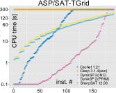
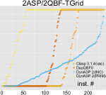
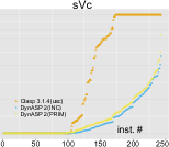
Figure 4: Results of randomly generated and selected real-world instances.

We state which parts of ${\mathsf{INC}}$ we adapt to compute the number of optimal answer sets in Algorithm 4 (#O${\mathsf{INC}}$). To slightly simplify the presentation of optimization rules, we assume without loss of generality that whenever an atom $a$ is introduced in bag $\chi(t)$ for some node $t$ of the TD, the optimization rule $r$, where $a$ occurs, belongs to the bag $\chi(t)$. First, we explain how to handle costs making use of function $\text{cst}(\Pi,M,A)$ as defined in Section 2. In a leaf (Line 1) we set the (current) cost to $0$. If we introduce an atom $a$ (Line 2–4) the cost depends on whether $a$ is set to true or false in $M$ and we add the cost of the “child” tuple. Removal of rules (Line 5–6) is trivial, as we only store the same values. If we remove an atom (Line 7–8), we compute the minimum costs only for tuples $\langle M^{-}_{a},\sigma,\mathcal{C},c,n\rangle$ where $c$ is minimal among $M^{-}_{a}$, $\sigma$, $\mathcal{C}$, that is, for a multiset $\mathcal{S}$ we let $\operatorname{kmin}(\mathcal{S})\,\mathrel{\mathop{:}}=\lbag\langle M^{-}_{a},\sigma,\mathcal{C},c,n\rangle\mid c=\min\{c^{\prime}:\langle M^{-}_{a},\sigma,\mathcal{C},c^{\prime},\cdot\rangle\in\mathcal{S}\},\langle M^{-}_{a},\sigma,\mathcal{C},c,n\rangle\in\mathcal{S}\rbag$. We require a multiset notation for counting (see below). If we join two nodes (Line 9–11), we compute the minimum value in the table of one child plus the minimum value of the table of the other child minus the value of the cost for the current bag, which is exactly the value we added twice. Next, we explain how to handle the number of witnessed sets that are minimal with respect to the cost. In a leaf (Line 1), we set the counter to $1$. If we introduce/remove a rule or introduce an atom (Line 2–6), we can simply take the number $n$ from the child. If we remove an atom (Line 7–8) we first obtain a multiset from computing $\operatorname{kmin}$, which can contain several tuples for $M^{-}_{a},\sigma,\mathcal{C},c$ as we obtained $M^{-}_{a}$ either from $M\setminus\{a\}$ if $a\in M$ or $M$ if $a\notin M$ giving rise multiple solutions, that is, $\operatorname{cnt}(\mathcal{S})\,\mathrel{\mathop{:}}=\{\langle M,\sigma,\mathcal{C},c,\sum_{\langle M,\sigma,\mathcal{C},c,n^{\prime}\rangle\in\mathcal{S}}n^{\prime}\rangle\mid\langle M,\sigma,\mathcal{C},c,n\rangle\in\mathcal{S}\}$. If we join nodes (Line 7–9), we multiply the number $n^{\prime}$ from the tuple of one child with the number $n^{\prime\prime}$ from the tuple of the other child, restrict results with respect to minimum costs, and sum up the resulting numbers.

Corollary 1.

Given a program $\Pi$, algorithm ${\#O{\mathsf{INC}}}$ runs in time ${\mathcal{O}}(log(m)\cdot 2^{2^{k+2}\cdot\ell^{k+1}}\|I(\Pi)\|^{2})$, where $k\,\mathrel{\mathop{:}}=\mathit{tw}(I(\Pi))$, $\ell\,\mathrel{\mathop{:}}=max\{3,\operatorname{bnd}(r):r\in\operatorname{WGT}(\Pi)\}$, and $m\,\mathrel{\mathop{:}}=\Sigma_{r\in\operatorname{OPT}(\Pi)}\operatorname{wght}(r)$.

4 Experimental Evaluation

We implemented the algorithms ${{\mathcal{DP}}_{{\mathsf{PRIM}}}}$ and ${{\mathcal{DP}}_{{\mathsf{INC}}}}$ into a prototypical solver $\mbox{\text{DynASP2}}(\cdot)$ and performed experiments to evaluate its runtime behavior. Clearly, we cannot hope to solve programs with graph representations of high treewidth. However, programs involving real-world graphs such as graph problems on transit graphs admit TDs of small width. We used both random and structured instances for our benchmarks. We refer to Appendix C for instance, machine and solver configurations and descriptions. The random instances (Sat-TGrid, 2QBF-TGrid, ASP-TGrid, 2ASP-TGrid) were designed to have a high number of variables and solutions and treewidth at most three. The structured instances model various graph problems (2Col, 3Col, Ds, St cVc, sVc) on real world mass transit graphs. For a graph, program 2Col counts all 2-colorings, 3Col counts all 3-colorings, Ds counts all minimal dominating sets, St counts all Steiner trees, cVc counts all cardinality-minimal vertex covers, and sVc counts all subset-minimal vertex covers.

	2Col		3Col		Ds		St		cVc		sVc
Clasp(usc)	31.72	(21)	0.10	(0)	8.99	(3)	0.21	(0)	29.88	(21)	98.34	(71)
DynASP2(PRIM)	1.54	(0)	0.53	(0)	0.68	(0)	79.36	(221)	0.99	(0)	1.30	(0)
DynASP2(INC)	1.43	(0)	0.58	(0)	0.54	(0)	115.02	(498)	0.68	(0)	0.78	(0)

Table 1: Runtimes (given in sec.; #timeouts in brackets) on real-world instances.

In order to draw conclusions about the efficiency of DynASP2, we mainly inspected the cpu running time and number of timeouts using the average over three runs per instance (three fixed seeds allow certain variance [1] for heuristic TD computation). We limited available memory (RAM) to 4GB (to run SharpSAT on large instances), and cpu time to 300 seconds, and then compared DynASP2 with the dedicated #SAT solvers SharpSAT [20] and Cachet [18], the QBF solver DepQBF0, and the ASP solver Clasp [9]. Figure 4 illustrates runtime results as a cactus plot. Table 1 reports on the average running times, numbers of solved instances and timeouts on the structured instance sets.

Summary.

Our empirical benchmark results confirm that DynASP2 exhibits competitive runtime behavior if the input instance has small treewidth. Compared to state-of-the-art Asp and Qbf solvers, DynASP2 has an advantage in case of many solutions, whereas Clasp and DepQBF0 perform well if the number of solutions is relatively small. However, DynASP2 is still reasonably fast on structured instances with few solutions as it yields the result mostly within less than 10 seconds. We observed that ${\mathsf{INC}}$ seems to be the better algorithm in our setting, indicating that the smaller width obtained by decomposing the incidence graph generally outweighs the benefits of simpler solving algorithms for the primal graph. However, if ${\mathsf{INC}}$ and ${\mathsf{PRIM}}$ run with graphs of similar width, ${\mathsf{PRIM}}$ benefits from its simplicity. A comparison to existing #SAT solvers suggests that, on random instances, they have a lower overhead (which is not surprising, since our algorithms are built for ASP), but, after about 150 seconds, our algorithms were still able to solve more instances than all other #SAT competitors.

5 Conclusion

In this paper, we presented novel DP algorithms for ASP, extending previous work [11] in order to cover the full ASP syntax. Our algorithms are based on two graph representations of programs and run in linear time with respect to the treewidth of these graphs and weights used in the program. Experiments indicate that our approach seems to be suitable for practical use, at least for certain classes of instances with low treewidth, and hence could fit into a portfolio-based solver.

Appendix A Additional Examples

In the following example, we briefly describe how we compute counterwitnesses using Algorithm 3 ($\mathsf{INC}$) for selected interesting cases. The example is similar to Example 6, which, however, describes handling counterwitnesses for Algorithm $\mathsf{PRIM}$.

Example 10.

We consider $\Pi$ of Example 1 and ${\cal T}^{\prime}=(\cdot,\chi)$ of Figure 3 and explain how we compute tables $\tau_{1}$, $\ldots$, $\tau_{18}$ in Figure 3 (right) using $\mathcal{DP}_{\mathsf{INC}}$. Table $\tau_{1}=\langle\emptyset,\emptyset,\emptyset\rangle$ as $\operatorname{type}(t_{1})=\textit{leaf}$. Node $t_{2}$ introduces atom $c$, resulting in table $\{\langle\{c\},\emptyset,\{(\emptyset,\emptyset)\}\rangle,\langle\emptyset,\emptyset,\emptyset\rangle\}$. Then, node $t_{3}$ introduces rule $r_{1}$ and node $t_{4}$ introduces rule $r_{2}$. As a result, table $\tau_{4}$ additionally contains computed rule-states (see $\operatorname{SatRules}$) for witnesses and counterwitnesses of $\tau_{3}$. Node $t_{5}$ introduces atom $b$, while $t_{6}$ removes $b$. Next, we focus on table $\tau_{6}$, since rule-states for counterwitnesses require updates for choice rule $r_{1}$ (see $\operatorname{UpdtWgt\&Ch}$). Witness $M_{6.2}=\{c\}$ is obtained by extending some witness $M_{5.i}\supseteq\{b\}$ of $\tau_{5}$. For counterwitness $C_{6.2.1}=\{c\}$ we require to remember $\sigma_{6.2.1}(r_{1})=1$ (see $\operatorname{UpdtWgt\&Ch}$), since $t_{6}$ removes $b$ and $C_{6.2.1}$ stems from some $C_{5.i.{j_{1}}}$ with $b\not\in C_{5.i.{j_{1}}}$. The set $C_{5.i.{j_{1}}}$ cannot be a model of the GL reduct ${\{r_{1}\}}^{M_{5.i}}$ unless $r_{1}$ is satisfied because of its body, since $b\in M_{5.i}$ and $b\not\in C_{5.i.{j_{1}}}$. For choice rule $r_{1}$, $\sigma_{6.2.1}(r_{1})\neq\infty$ and $\sigma_{6.2.1}(r_{1})\neq 0$ indicates that we can satisfy $r_{1}$ only by $B^{+}(r_{1})\setminus M\neq\emptyset$ (see ${\cal P}\cup\{\cdots,\rho(r)>0\}$ in Definition 2). The remaining counterwitness $C_{6.2.2}=\emptyset$ was obtained by some $C_{5.i.{j_{2}}}$ with $b\not\in C_{5.i.{j_{2}}}$, since $\sigma_{6.2.2}(r_{2})=0$). Further, $C_{6.2.3}=\emptyset$ stems from $C_{5.i.{j_{3}}}\supseteq\{b\}$, since $\sigma_{6.2.3}(r_{2})=1$.

Appendix B Omitted Proofs

B.1 Proof of Theorem 2 (Correctness result of $\mathsf{PRIM}$)

Proposition 1.

The algorithm ${\mathcal{DP}}_{{\mathsf{PRIM}}}$ is correct.

Proof (Sketch)..

Let $\Pi$ be the given program and $\mathcal{T}=(T,\chi)$ the TD, where $T=(N,\cdot,n)$. We obtain correctness by slightly modifying the proof of Theorem 2 as well as relevant definitions and propositions following Appendix B.2. More precisely, we drop the mappings $\sigma$ and relevant conditions for mappings $\sigma$ and replace them by satisfiability of the respective rules. By definition of a primal graph of a program, we know that for every rule $r\in\Pi$ there is a node $t\in N$ such that $\chi(t)\subseteq\text{at}(r)$. Hence, for a node $t$ we can decide satisfiability of a rule directly, if bag $\chi(t)$ contains all atoms of a rule, when computing the tables. We directly obtain completeness and soundness, which yields the proposition. ∎

Proposition 2.

Given a program $\Pi$ and a TD ${\cal T}=(T,\chi)$ of the primal graph $P(\Pi)$ of width $k$ with $T=(N,\cdot,\cdot)$. For every node $t\in N$, there are at most $2^{k+1}\cdot 2^{2^{k+1}}$ tuples in table $\tau_{t}$, which is constructed by algorithm ${\mathcal{DP}}_{{\mathsf{INC}}}$.

Proof.

Let $\Pi$ be a program, $P(\Pi)$ its primal graph, and $\mathcal{T}=(T,\chi)$ a TD of $P(\Pi)$ with $T=(N,\cdot,\cdot)$. For every node $t\in T$, we have by definition of a tree decomposition and its width a maximum bag size of $k+1$, i.e., $|\chi(t)|-1\leq k$. Therefore, we can have $2^{k+1}$ many witnesses and for each witness a subset of the set of witnesses consisting of at most $2^{2^{k+1}}$ many counterwitnesses. Consequently, there are at most $2^{k+1}\cdot 2^{2^{k+1}}$ tuples per node. Hence, the proposition is true. ∎

Now, we are in situation to prove Theorem 2.

Proof of Theorem 2..

Let $\Pi$ be a program, $I(\Pi)=(V,\cdot)$ its incidence graph, and $k$ be the treewidth of $P(\Pi)$. Proposition 1 establishes correctness. Then, we can compute in time $2^{{\mathcal{O}}(k^{3})}\cdot|V|$ a TD of width at most $k$ Bodlaender96. We take such a TD and compute in linear time a nice TD Kloks94a. Let $\mathcal{T}=(T,\chi)$ be such a nice TD with $T=(N,\cdot,n)$. Since the number of nodes in $N$ is linear in the graph size and since for every node $t\in N$ the table $\tau_{t}$ is bounded by $2^{k+1}\cdot 2^{2^{k+1}}$ according to Proposition 2, we obtain a running time of ${\mathcal{O}}(2^{2^{k+2}}\cdot\|P(\Pi)\|)$. Consequently, the theorem sustains. ∎

B.2 Proof of Theorem 3 (Correctness result of $\mathsf{INC}$)

In the following, we provide insights on the correctness of Algorithm 3 ($\mathsf{INC}$). The correctness proof of these algorithms need to investigate each node type separately. We have to show that a tuple at a node $t$ guarantees existence of a model for the program $\Pi_{\leq t}$, proving soundness. Conversely, one can show that each candidate answer set is indeed evaluated while traversing the TD, which provides completeness. We employ this idea using the notions of (i) partial solutions consisting of partial models and the notion of (ii) local partial solutions.

Definition 3.

Let $\Pi$ be a program, $\mathcal{T}=(T,\chi)$ be a TD of the incidence graph $I(\Pi)$ of $\Pi$, where $T=(N,\cdot,\cdot)$, and $t\in N$ be a node. Further, let ${M},C\subseteq\text{at}_{\leq t}$ be sets and ${\sigma}:\Pi_{\leq t}\rightarrow\mathbb{N}_{0}\cup\{\infty\}$ a mapping. The tuple $({C},{\sigma})$ is a partial model for $t$ under $M$ if the following conditions hold:

1. ${C}\vDash(\Pi_{<t})^{M}$,

2. for $r\in\Pi_{\leq t}$ we have ${\sigma}(r)=0$ or ${\sigma}(r)=\infty$,

3. 1. for $r\in\operatorname{DISJ}(\Pi_{\leq t})$ we have $B^{-}_{r}\cap M\neq\emptyset$ or $B^{+}_{r}\cap\text{at}_{\leq t}\not\subseteq C$ or $H_{r}\cap C\neq\emptyset$ if and only if $\sigma(r)=\infty$,

   2. for $r\in\operatorname{WGT}(\Pi_{\leq t})$ we have $\operatorname{wght}(r,(\text{at}(r)\setminus\text{at}_{\leq t})\cup(B^{-}_{r}\setminus M)\cup(B^{+}_{r}\cap C))<\operatorname{bnd}(r)$ or $H_{r}\cap C\neq\emptyset$ if and only if $\sigma(r)=\infty$, and

   3. for $r\in\operatorname{CH}(\Pi_{\leq t})$ we have $B^{-}_{r}\cap M\neq\emptyset$ or $B^{+}_{r}\cap\text{at}_{\leq t}\not\subseteq C$ or both $H_{r}\subseteq\text{at}_{\leq t}$ and $H_{r}\cap(M\setminus C)=\emptyset$ if and only if ${\sigma(r)}=\infty$.

Definition 4.

Let $\Pi$ be a program, $\mathcal{T}=(T,\chi)$ where $T=(N,\cdot,n)$ be a TD of $I(\Pi)$, and $t\in N$ be a node. A partial solution for $t$ is a tuple $({M},{\sigma},{{\cal C}})$ where $({M},{\sigma})$ is a partial model under $M$ and ${{\cal C}}$ is a set of partial models $({C},{\rho})$ under ${M}$ with ${C}\subsetneq{M}$.

The following lemma establishes correspondence between answer sets and partial solutions.

Lemma 1.

Let $\Pi$ be a program, $\mathcal{T}=(T,\chi)$ be a TD of the incidence graph $I(\Pi)$ of program $\Pi$, where $T=(\cdot,\cdot,n)$, and $\chi(n)=\emptyset$. Then, there exists an answer set ${M}$ for $\Pi$ if and only if there exists a partial solution $u=({M},\sigma,\emptyset)$ with $\sigma^{-1}(\infty)=\Pi$ for root $n$.

Proof.

Given an answer set ${M}$ of $\Pi$ we construct $u=({M},{\sigma},\emptyset)$ with ${\sigma}(r)\,\mathrel{\mathop{:}}=\infty$ for $r\in\Pi$ such that $u$ is a partial solution for $n$ (according to Definition 4). For the other direction, Definitions 3 and 4 guarantee that ${M}$ is an answer set if there exists some tuple $u$. In consequence, the lemma holds. ∎

Next, we require the notion of local partial solutions corresponding to the tuples obtained in Algorithm 3.

Definition 5.

Let $\Pi$ be a program, $\mathcal{T}=(T,\chi)$ a TD of $I(\Pi)$, where $T=(N,\cdot,n)$, $t\in N$ be a node, ${M},C\subseteq\text{at}(\Pi)$ sets, and ${\sigma}:\Pi\rightarrow\mathbb{N}_{0}\cup\{\infty\}$ be a mapping. We define the local rule-state $\sigma^{t,M,C}\,\mathrel{\mathop{:}}=({\sigma}\squplus\sigma^{\prime})^{-}_{\Pi_{<t}}$ for ${C}$ under $M$ of node $t$ where $\sigma^{\prime}:\Pi_{t}\rightarrow\mathbb{N}_{0}\cup\{\infty\}$ by

$$\sigma^{\prime}(r)\,\mathrel{\mathop{:}}=\begin{cases}\operatorname{wght}(r,(\text{at}_{\leq t}\setminus\chi(t))\cap[(B^{-}_{r}\setminus{M})\cup(B^{+}_{r}\cap{C})])&r\in\operatorname{WGT}(\Pi_{t})\\ \left|(\text{at}_{\leq t}\setminus\chi(t))\cap H_{r}\cap({M}\setminus C)\right|&r\in\operatorname{CH}(\Pi_{t})\end{cases}$$

Definition 6.

Let $\Pi$ be a program, $\mathcal{T}=(T,\chi)$ a TD of the incidence graph $I(\Pi)$, where $T=(N,\cdot,n)$, and $t\in N$ be a node. A tuple $u=\langle M,\sigma,{\cal C}\rangle$ is a local partial solution for $t$ if there exists a partial solution ${\hat{}u}=({\hat{M}},{\hat{\sigma}},{\hat{\cal C}})$ for $t$ such that the following conditions hold:

1. $M={\hat{M}}\cap\chi(t)$,

2. $\sigma={\hat{\sigma}}^{t,{\hat{M}},{\hat{M}}}$, and

3. ${\cal C}=\{\langle{\hat{C}}\cap\chi(t),{\hat{\rho}}^{t,{\hat{M}},{\hat{C}}}\rangle\mid({\hat{C}},{\hat{\rho}})\in{\hat{\cal C}}\}$.

We denote by ${\hat{}u}^{t}$ the local partial solution $u$ for $t$ given partial solution ${\hat{}u}$.

The following proposition provides justification that it suffices to store local partial solutions instead of partial solutions for a node $t\in N$.

Lemma 2.

Let $\Pi$ be a program, $\mathcal{T}=(T,\chi)$ a TD of $I(\Pi)$, where $T=(N,\cdot,n)$, and $\chi(n)=\emptyset$. Then, there exists an answer set for $\Pi$ if and only if there exists a local partial solution of the form $\langle\emptyset,\emptyset,\emptyset\rangle$ for the root $n\in N$.

Proof.

Since $\chi(n)=\emptyset$, every partial solution for the root $n$ is an extension of the local partial solution $u$ for the root $n\in N$ according to Definition 6. By Lemma 1, we obtain that the lemma is true. ∎

In the following, we abbreviate atoms occurring in bag $\chi(t)$ by $\text{at}_{t}$, i.e., $\text{at}_{t}\,\mathrel{\mathop{:}}=\chi(t)\setminus\Pi_{t}$.

Proposition 3 (Soundness).

Let $\Pi$ be a program, $\mathcal{T}=(T,\chi)$ a TD of incidence graph $I(\Pi)$, where $T=(N,\cdot,\cdot)$, and $t\in N$ a node. Given a local partial solution $u^{\prime}$ of child table $\tau^{\prime}$ (or local partial solution $u^{\prime}$ of table $\tau^{\prime}$ and local partial solution $u^{\prime\prime}$ of table $\tau^{\prime\prime}$), each tuple $u$ of table $\tau_{t}$ constructed using table algorithm ${\mathsf{INC}}$ is also a local partial solution.

Proof.

Let $u^{\prime}$ be a local partial solution for $t^{\prime}\in N$ and $u$ a tuple for node $t\in N$ such that $u$ was derived from $u^{\prime}$ using table algorithm ${\mathsf{INC}}$. Hence, node $t^{\prime}$ is the only child of $t$ and $t$ is either removal or introduce node.

Assume that $t$ is a removal node and $r\in\Pi_{t^{\prime}}\setminus\Pi_{t}$ for some rule $r$. Observe that $u=\langle M,\sigma,{\cal C}\rangle$ and $u^{\prime}=\langle M,\sigma^{\prime},{\cal C^{\prime}}\rangle$ are the same in witness $M$. According to Algorithm 3 and since $u$ is derived from $u^{\prime}$, we have $\sigma^{\prime}(r)=\infty$. Similarly, for any $\langle C^{\prime},\rho^{\prime}\rangle\in{\cal C^{\prime}}$, $\rho^{\prime}(r)=\infty$. Since $u^{\prime}$ is a local partial solution, there exists a partial solution ${\hat{}u^{\prime}}$ of $t^{\prime}$, satisfying the conditions of Definition 6. Then, ${\hat{}u^{\prime}}$ is also a partial solution for node $t$, since it satisfies all conditions of Definitions 3 and 4. Finally, note that $u=({\hat{u}^{\prime}})^{t}$ since the projection of ${\hat{}u^{\prime}}$ to the bag $\chi(t)$ is $u$ itself. In consequence, the tuple $u$ is a local partial solution.

For $a\in\text{at}_{t^{\prime}}\setminus\text{at}_{t}$ as well as for introduce nodes, we can analogously check the proposition.

Next, assume that $t$ is a join node. Therefore, let $u^{\prime}$ and $u^{\prime\prime}$ be local partial solutions for $t^{\prime},t^{\prime\prime}\in N$, respectively, and $u$ be a tuple for node $t\in N$ such that $u$ can be derived using both $u^{\prime}$ and $u^{\prime\prime}$ in accordance with the ${\mathsf{INC}}$ algorithm. Since $u^{\prime}$ and $u^{\prime\prime}$ are local partial solutions, there exists partial solution ${\hat{}u^{\prime}}=({\hat{M}^{\prime}},{\hat{\sigma}^{\prime}},{\hat{\cal C^{\prime}}})$ for node $t^{\prime}$ and partial solution ${\hat{}u^{\prime\prime}}=({\hat{M}^{\prime\prime}},{\hat{\sigma}^{\prime\prime}},{\hat{\cal C^{\prime\prime}}})$ for node $t^{\prime\prime}$. Using these two partial solutions, we can construct ${\hat{}u}=({\hat{M}^{\prime}}\cup{\hat{M}^{\prime\prime}},{\hat{\sigma}^{\prime}}\squplus{\hat{\sigma}^{\prime\prime}},{\hat{\cal C^{\prime}}}\bowtie{\hat{\cal C^{\prime\prime}}})$ where $\bowtie(\cdot,\cdot)$ is defined in accordance with Algorithm 3 as follows:

$${\hat{\cal C^{\prime}}}\bowtie{\hat{\cal C^{\prime\prime}}}\,\mathrel{\mathop{:}}= \{({\hat{C}^{\prime}}\cup{\hat{C}^{\prime\prime}},{\hat{\rho}^{\prime}}\squplus{\hat{\rho}^{\prime\prime}})\mid({\hat{C}^{\prime}},{\hat{\rho}^{\prime}})\in{\hat{\cal C^{\prime}}},({\hat{C}^{\prime\prime}},{\hat{\rho}^{\prime\prime}})\in{\hat{\cal C^{\prime\prime}}},{\hat{C}^{\prime}}\cap\text{at}_{t}={\hat{C}^{\prime\prime}}\cap\text{at}_{t}\}\cup$$

$$\{({\hat{C}^{\prime}}\cup{\hat{M}^{\prime\prime}},{\hat{\rho}^{\prime}}\squplus{\hat{\sigma}^{\prime\prime}})\mid({\hat{C}^{\prime}},{\hat{\rho}^{\prime}})\in{\hat{\cal C^{\prime}}},{\hat{C}^{\prime}}\cap\text{at}_{t}={\hat{M}^{\prime\prime}}\cap\text{at}_{t}\}\cup$$

$$\{({\hat{M}^{\prime}}\cup{\hat{C}^{\prime\prime}},{\hat{\sigma}^{\prime}}\squplus{\hat{\rho}^{\prime\prime}})\mid({\hat{C}^{\prime\prime}},{\hat{\rho}^{\prime\prime}})\in{\hat{\cal C^{\prime\prime}}},{\hat{M}^{\prime}}\cap\text{at}_{t}={\hat{C}^{\prime\prime}}\cap\text{at}_{t}\}.$$

Then, we check all conditions of Definitions 3 and 4 in order to verify that ${\hat{}u}$ is a partial solution for $t$. Moreover, the projection ${\hat{}u}^{t}$ of ${\hat{}u}$ to the bag $\chi(t)$ is exactly $u$ by construction and hence, $u={\hat{}u}^{t}$ is a local partial solution.

Since we have provided arguments for each node type, we established soundness in terms of the statement of the proposition.

∎

Proposition 4 (Completeness).

Let $\Pi$ be a program, $\mathcal{T}=(T,\chi)$ where $T=(N,\cdot,\cdot)$ be a TD of $I(\Pi)$ and $t\in N$ be a node. Given a local partial solution $u$ of table $\tau_{t}$, either $t$ is a leaf node, or there exists a local partial solution $u^{\prime}$ of child table $\tau^{\prime}$ (or local partial solution $u^{\prime}$ of table $\tau^{\prime}$ and local partial solution $u^{\prime\prime}$ of table $\tau^{\prime\prime}$) such that $u$ can be constructed by $u^{\prime}$ (or $u^{\prime}$ and $u^{\prime\prime}$, respectively) and using table algorithm ${{\mathsf{INC}}}$.

Proof.

Let $t\in N$ be a removal node and $r\in\Pi_{t^{\prime}}\setminus\Pi_{t}$ with child node $t^{\prime}\in N$. We show that there exists a tuple $u^{\prime}$ in table $\tau_{t^{\prime}}$ for node $t^{\prime}$ such that $u$ can be constructed using $u^{\prime}$ by ${\mathsf{INC}}$ (Algorithm 3). Since $u$ is a local partial solution, there exists a partial solution ${\hat{}u}=({\hat{M}},{\hat{\sigma}},{\hat{\cal C}})$ for node $t$, satisfying the conditions of Definition 6. Since $r$ is the removed rule, we have ${\hat{\sigma}}(r)=\infty$. By similar arguments, we have $\hat{\rho}(r)=\infty$ for any tuple $({\hat{C}},{\hat{\rho}})\in{\hat{\cal C}}$. Hence, ${\hat{}u}$ is also a partial solution for $t^{\prime}$ and we define $u^{\prime}\,\mathrel{\mathop{:}}={\hat{}u}^{t^{\prime}}$, which is the projection of ${\hat{}u}$ onto the bag of $t^{\prime}$. Apparently, the tuple $u^{\prime}$ is a local partial solution for node $t^{\prime}$ according to Definition 6. Then, $u$ can be derived using ${\mathsf{INC}}$ algorithm and $u^{\prime}$. By similar arguments, we establish the proposition for $a\in\text{at}_{t^{\prime}}\setminus\text{at}_{t}$ and the remaining (three) node types. Hence, the propositions sustains. ∎

Now, we are in situation to prove Theorem 3.

Proof of Theorem 3..

We first show soundness. Let $\mathcal{T}=(T,\chi)$ be the given TD, where $T=(N,\cdot,n)$. By Lemma 2 we know that there is an answer set for $\Pi$ if and only if there exists a local partial solution for the root $n$. Note that the tuple is of the form $\langle\emptyset,\emptyset,\emptyset\rangle$ by construction. Hence, we proceed by induction starting from the leaf nodes. In fact, the tuple $\langle\emptyset,\emptyset,\emptyset\rangle$ is trivially a partial solution by Definitions 3 and 4 and also a local partial solution of $\langle\emptyset,\emptyset,\emptyset\rangle$ by Definition 6. We already established the induction step in Proposition 3. Hence, when we reach the root $n$, when traversing the TD in post-order by Algorithm $\mathcal{DP}_{{\mathsf{INC}}}$, we obtain only valid tuples inbetween and a tuple of the form $\langle\emptyset,\emptyset,\emptyset\rangle$ in the table of the root $n$ witnesses an answer set. Next, we establish completeness by induction starting from the root $n$. Let therefore, $M$ be an arbitrary answer set of $\Pi$. By Lemma 2, we know that for the root $n$ there exists a local partial solution of the form $\langle\emptyset,\emptyset,\emptyset\rangle$ for partial solution $\langle M,\sigma,\emptyset\rangle$ with $\sigma(r)=\infty$ for $r\in\Pi$. We already established the induction step in Proposition 4. Hence, we obtain some (corresponding) tuples for every node $t$. Finally, stopping at the leaves $n$. In consequence, we have shown both soundness and completeness resulting in the fact that Theorem 3 is true. ∎

Theorem 3 states that we can decide the problem Cons by means of Algorithm $\mathcal{DP}_{{\mathsf{INC}}}$, which uses Algorithm 3.

B.3 Proof of Theorem 4 (Worst-case Runtime Bounds of $\mathsf{INC}$)

First, we give a proposition on worst-case space requirements in tables for the nodes of our algorithm.

Proposition 5.

Given a program $\Pi$, a TD ${\cal T}=(T,\chi)$ with $T=(N,\cdot,\cdot)$ of the incidence graph $I(\Pi)$, and a node $t\in N$. Then, there are at most $2^{k+1}\cdot\ell^{k+1}\cdot 2^{2^{k+1}\cdot\ell^{k+1}}$ tuples in $\tau_{t}$ using algorithm ${\mathcal{DP}}_{{\mathsf{INC}}}$ for width $k$ of ${\cal T}$ and bound $\ell=max\{3,\operatorname{bnd}(r):r\in\operatorname{WGT}(\Pi)\}$.

Proof (Sketch)..

Let $\Pi$ be the given program, ${\cal T}=(T,\chi)$ a TD of the incidence graph $I(\Pi)$, where $T=(N,\cdot,\cdot)$, and $t\in N$ a node of the TD. Then, by definition of a decomposition of the primal graph for each node $t\in N$, we have $|\chi(t)|-1\leq k$. In consequence, we can have at most $2^{k+1}$ many witnesses, and for each witness a subset of the set of witnesses consisting of at most $2^{2^{k+1}}$ many counterwitnesses. Moreover, we observe that Algorithm 3 can be easily modified such that a state $\sigma:\Pi_{t}\rightarrow\mathbb{N}_{0}\cup\{\infty\}$ for node $t\in N$ assigns each weight rule $r\in\operatorname{WGT}(\Pi)$ a non-negative integer $\sigma(r)\leq\operatorname{bnd}(r)+1$, each choice rule $r\in\operatorname{CH}(\Pi)$ a non-negative integer $\sigma(r)\leq 2$ and each disjunctive rule $r\in\operatorname{DISJ}(\Pi)$ a non-negative integer $\sigma(r)\leq 1$. This is the case since we need to model $\sigma(r)=0$ and $\sigma(r)=\infty$ for each disjunctive rule $r$. Moreover, for choice rules $r$, it suffices to additionally model whether $1\leq\sigma(r)<\infty$, and for weight rules $r$, we require to remember any weight $1\leq\sigma(r)\leq\operatorname{bnd}(r)$. In total, we need to distinguish $\ell^{k+1}$ different rule-states for each witness of a tuple in the table $\tau_{t}$ for node $t$. Since for each witness in the table $\tau_{t}$ for node $t\in N$ we remember rule-states for at most $k+1$ rules, we store up to $\ell^{k+1}$ many combinations per witness. In total we end up with at most $2^{2^{k+1}\cdot\ell^{k+1}}$ many counterwitnesses for each witness and rule-state in the worst case. Thus, there are at most $2^{k+1}\cdot\ell^{k+1}\cdot 2^{2^{k+1}\cdot\ell^{k+1}}$ tuples in table $\tau_{t}$ for node $t$. In consequence, we established the proposition. ∎

Proof of Theorem 4..

Let $\Pi$ be a program, $I(\Pi)=(V,\cdot)$ its incidence graph, and $k$ be the treewidth of $P(\Pi)$. Then, we can compute in time $2^{{\mathcal{O}}(k^{3})}\cdot|V|$ a TD of width at most $k$ Bodlaender96. We take such a TD and compute in linear time a nice TD Kloks94a. Let $\mathcal{T}=(T,\chi)$ be such a nice TD with $T=(N,\cdot,\cdot)$. Since the number of nodes in $N$ is linear in the graph size and since for every node $t\in N$ the table $\tau_{t}$ is bounded by $2^{k+1}\cdot\ell^{k+1}\cdot 2^{2^{k+1}\cdot\ell^{k+1}}$ according to Proposition 5, we obtain a running time of ${\mathcal{O}}(2^{2^{k+2}\cdot\ell^{k+1}}\|I(\Pi)\|)$. Consequently, the theorem sustains. ∎

B.4 Correctness of the Algorithm $\mathcal{DP}_{{\#O{\mathsf{INC}}}}$

The following propositions states that we can use Algorithm $\mathcal{DP}_{{\#O{\mathsf{INC}}}}$ to actually count optimal answer sets.

Proposition 6.

The algorithm $\mathcal{DP}_{{\#O{\mathsf{INC}}}}$ is correct.

Proof (Sketch)..

We follow the proof of Theorem 3. First, we additionally need to take care of the optimization rules obtained by extending Definitions 3–6, the lemmas and propositions accordingly. In order to handle the counting, we have to extend Definitions 3–6 by counters. Further, we additionally need to ensure and prove in the induction steps, which are established by Propositions 3 and 4, that any fixed partial solution is obtained from child to parent via a corresponding local partial solution by the algorithm. ∎

Appendix C Experiments

C.1 Solvers

The solvers tested include our own prototypical implementation, which we refer to as DynASP, and the existing solvers

• Cachet 1.21 [18], which is a SAT model counter,

• DepQBF0 , which is the solver DepQBF LonsingBiere10 where we added a naive implementation using methods described by Lonsing Lonsing15,

• Clasp 3.1.4 GebserKaufmannSchaub12a, which is an ASP solver, and

• SharpSAT 12.08 [20], which is a SAT model counter.

C.2 Environment

We ran the experiments on an Ubuntu 12.04 Linux cluster of 3 nodes with two AMD Opteron 6176 SE CPUs of 12 physical cores each at 2.3Ghz clock speed and 128GB RAM. Input instances were given to the solvers via shared memory. All solvers have been compiled with gcc version 4.9.3. Available memory was limited to 4GB RAM, which was necessary to run SharpSAT on larger instances, and CPU time to 300 seconds. We used default options for cachet and SharpSAT, “–qdc” for DepQBF0, “–stats=2 –opt-mode=optN -n 0 –opt-strategy=usc -q” and no solution printing/recording for clasp. We also benchmarked clasp with the flag “bb”. However, “usc” outperformed “bb” on all our benchmarks. All solvers have been executed in single core mode.

C.3 Instances

We used both random and structured instances for benchmark sets, which we briefly describe below. The benchmark sets, including instances and encodings, as well as results are available online on github.

The random instances (Sat-TGrid, 2QBF-TGrid, ASP-TGrid, 2ASP-TGrid) were designed to have a high number of variables and solutions and treewidth at most three. The instances are constructed as follows: Let $k$ and $\ell$ be some positive integers and $p$ a rational number such that $0<p\leq 1$. An instance $F$ of Sat-TGrid$(k,l,p)$ consists of the set $V=\{(1,1),\ldots,(1,\ell),(2,\ell),\ldots,(k,\ell)\}$ of variables and with probability $p$ for each variable $(i,j)$ such that $1<i\leq k$ and $1<j\leq\ell$ a clause $s_{1}(i,j)$, $s_{2}(i-1,j)$, $s_{3}(i,j-1)$, a clause $s_{4}(i,j)$, $s_{5}(i-1,j)$, $s_{6}(i-1,j-1)$, and a clause $s_{7}(i,j)$, $s_{8}(i-1,j-1)$, $s_{9}(i,j-1)$ where $s_{i}\in\{-,+\}$ is selected with probability one half. In that way, such an instance has an underlying dependency graph that consists of various triangles forming for probability $p=1$ a graph that has a grid as subgraph. Let $q$ be a rational number such that $0<q\leq 1$. An instance of the set 2Qbf-TGrid$(k,l,p,q)$ is of the form $\exists V_{1}.\forall V_{2}.F$ where a variable belongs to $V_{1}$ with probability $q$ and to $V_{2}$ otherwise. Instances of the sets ASP-TGrid or 2ASP-TGrid have been constructed in a similar way, however, as an Asp program instead of a formula. Note that the number of answer sets and the number of satisfiable assignments correspond. We fixed the parameters to $p=0.85$, $k=3$, and $l\in\{40,80,\ldots,400\}$ to obtain instances that have with high probability a small fixed width, a high number of variables and solutions. Further, we took fixed random seeds and generated 10 instances to ensure a certain randomness.

The structured instances model various graph problems (2Col, 3Col, Ds, St cVc, sVc) on real world mass transit graphs of 82 cities, metropolitan areas, or countries. The graphs were extracted from publicly available mass transit data feeds gtfs using gtfs2graphs Fichte16c and split by transportation type, e.g., train, metro, tram. We excluded bus networks as size and treewidth were too large. For an input graph, the 2Col encoding counts all minimal sets $S$ of vertices s.t. there are two sets $F$ and $S$ where no two neighboring vertices $v$ and $w$ belong to $F$; 3Col counts all 3-colorings; Ds counts all minimal dominating sets; St counts all Steiner trees; cVc counts all minimal vertex covers; and sVc counts all subset-minimal vertex covers. Since we cannot expect to solve instances of high treewidth efficiently, we restricted the instances to those where we were able to find decompositions of width below 20 within 60 seconds.

C.4 Extended Discussion on the Results

In order to draw conclusions about the efficiency of our approach, we mainly inspected the total cpu running time and number of timeouts on the random and structured benchmark sets. Note that we did not record I/O times. The runtime for $\mbox{\text{DynASP2}}(\cdot)$ includes decomposition times using heuristics from Dell16b,DermakuEtAl08. We randomly generated three fixed seeds for the decomposition computation to allow a certain variance [1]. When evaluating the results, we took the average over the three runs per instance. Figure 4 illustrates solver runtime on the various random instance sets and a selected structured instance set as a cactus plot. Table 1 reports on the average running times, number of solved instances, and number of timeouts of the solvers on the structured instance sets.

C.4.1 Results.

SAT-TGrid and Asp-TGrid: Cachet solved 125 instances. Clasp always timed out. A reason could be the high number of solutions as Clasp counts the models by enumerating them (without printing them). $\mbox{\text{DynASP2}}(\cdot)$ solved each instance within at most 270 seconds (on average 67 seconds). The best configuration with respect to runtime was $\mathsf{PRIM}$. However, the running times of the different configurations were close. We observed as expected a sub-polynomial growth in the runtime with an increasing number of solutions. SharpSAT timed out on 3 instances and ran into a memory out on 7 instances, but solved most of the instances quite fast. Half of the instances were solved within 1 second and more than 80% of the instances within 10 seconds, and about 9% of the instances took more than 100 seconds. The number of solutions does not have an impact on the runtime of SharpSAT. SharpSAT was the fastest solver in total. However, $\mbox{\text{DynASP2}}(\cdot)$ solved all instances. The results are illustrated in the two left graphs of Figure 4.

2QBF-TGrid and 2ASP-TGrid: Clasp solved more than half of the instances in less than 1 second, however, timed out on 59 instances. DepQBF0 shows a similar behavior as Clasp, which is not surprising as both solvers count the number of solutions by enumerating them and hence the number of solutions has a significant impact on the runtime of the solver. However, Clasp is faster throughout than DepQBF0. DynASP2($\mathsf{INC}$) solved half of the instances within less than 1 second, about 92% of the instances within less than 10 seconds, and provided solutions also if the instance had a large number of answer sets. DynASP2($\mathsf{PRIM}$) quickly produced timeouts due to large rules in program that produced a significantly larger width of the computed decompositions.

Structured instances: Clasp solved most of the structured instances reasonably fast. However, the number of solutions has again, similar to the random setting, a significant impact on its performance. If the number of solutions was very high, then Clasp timed out. If the instance has a small number of solutions, then Clasp yields the number almost instantly. However, $\mbox{\text{DynASP2}}(\cdot)$ also provided a solution within a second. $\mbox{\text{DynASP2}}(\cdot)$ solved for each set but the set St more than 80% of the instances in less than 1 second and the remaining instances in less than 100 seconds. For St the situation was different. Half of the instances were solved in less than 10 seconds and a little less than the other half timed out. Similar to the random setting, $\mbox{\text{DynASP2}}(\cdot)$ ran still fast on instances with a large number of solutions.

plain references_appendix

References

- [1] M. Abseher, F. Dusberger, N. Musliu, and S. Woltran. Improving the efficiency of dynamic programming on tree decompositions via machine learning. In IJCAI’15, 2015.
- [2] H. Bodlaender and A. M. C. A. Koster. Combinatorial optimization on graphs of bounded treewidth. The Computer Journal, 51(3):255–269, 2008.
- [3] G. Brewka, T. Eiter, and M. Truszczyński. Answer set programming at a glance. Communications of the ACM, 54(12):92–103, 2011.
- [4] F. Calimeri, W. Faber, M. Gebser, G. Ianni, R. Kaminski, T. Krennwallner, N. Leone, F. Ricca, and T. Schaub. ASP-core-2 input language format, 2013.
- [5] M. Cygan, F. V. Fomin, L. Kowalik, D. Lokshtanov, D. Marx, M. Pilipczuk, and S. Saurabh. Parameterized Algorithms. Springer, 2015.
- [6] A. Durand, M. Hermann, and P. G. Kolaitis. Subtractive reductions and complete problems for counting complexity classes. Th. Comput. Sc., 340(3), 2005.
- [7] Johannes K. Fichte and Stefan Szeider. Backdoors to tractable answer-set programming. AIJ, 220(0):64–103, 2015. Extended and updated version of a paper that appeared in Proc. of the 22nd International Conference on Artificial Intelligence (IJCAI’11).
- [8] M. Gebser, J. Bomanson, and T. Janhunen. Rewriting optimization statements in answer-set programs. Technical Communications of ICLP 2016, 2016.
- [9] M. Gebser, B. Kaufmann, and T. Schaub. Conflict-driven answer set solving: From theory to practice. AIJ, 187–188, 2012.
- [10] M. Hermann and R. Pichler. Complexity of counting the optimal solutions. Th. Comput. Sc., 410(38–40), 2009.
- [11] M. Jakl, R. Pichler, and S. Woltran. Answer-set programming with bounded treewidth. In IJCAI’09, volume 2, 2009.
- [12] C. Koch and N. Leone. Stable model checking made easy. In IJCAI’99, 1999.
- [13] V. Lifschitz. What is answer set programming? In AAAI’08, 2008.
- [14] R. Niedermeier. Invitation to Fixed-Parameter Algorithms. Oxford Univ. Pr., 2006.
- [15] R. Pichler, S. Rümmele, S. Szeider, and S. Woltran. Tractable answer-set programming with weight constraints: bounded treewidth is not enough. Theory Pract. Log. Program., 14(2), 2014.
- [16] N. Robertson and P.D. Seymour. Graph minors. II. algorithmic aspects of tree-width. J. Alg., 7(3):309–322, 1986.
- [17] M. Samer and S. Szeider. Algorithms for propositional model counting. J. Discrete Algorithms, 8(1), 2010.
- [18] T. Sang, F. Bacchus, P. Beame, H. A. Kautz, and T. Pitassi. Combining component caching and clause learning for effective model counting. In SAT’04, 2004.
- [19] T. Syrjänen. Lparse 1.0 user’s manual. tcs.hut.fi/Software/smodels/lparse.ps, 2002.
- [20] M. Thurley. sharpSAT – counting models with advanced component caching and implicit BCP. In SAT’06, 2006.