Abstract

We study the evolution in discrete time of certain age-structured populations, such as adults and juveniles, with a Ricker fitness function. We determine conditions for the convergence of orbits to the origin (extinction) in the presence of the Allee effect and time-dependent vital rates. We show that when stages interact, they may survive in the absence of interior fixed points, a surprising situation that is impossible without inter-stage interactions. We also examine the shift in the interior Allee equilibrium caused by the occurrence of interactions between stages and find that the extinction or Allee threshold does not extend to the new boundaries set by the shift in equilibrium, i.e. no interior equilibria are on the extinction threshold.

1 Introduction

The evolution of certain types of biological populations from a period, or time interval, $n$ to the next may be modeled by the discrete system

$$x_{n+1} =s_{n}x_{n}+s_{n}^{\prime}y_{n}$$ (1)

$$y_{n+1} =x_{n}^{\lambda}e^{r_{n}-bx_{n+1}-cx_{n}}$$ (2)

where $\lambda,c>0$, $b\geq 0$ with $s_{n}\in[0,1)$, $s_{n}^{\prime}\in(0,1]$ and $r_{n}\in(-\infty,\infty)$ for all $n$.

A common example is the population of a single species whose members are differentiated by their age group, where, e.g. $x_{n}$ and $y_{n}$ represent, respectively the population densities of adults and juveniles in time period $n$. In this setting, $s_{n}$ and $s_{n}^{\prime}$ denote the survival rates of adults and juveniles, respectively. For examples of stage-structured models, see [7] and [14] and references thereof.

The time dependent parameters $r_{n},s_{n},s_{n}^{\prime}$ may be periodic in the presence of periodic factors such as seasonal variations in the environment, migration, harvesting, predation, etc. The effects of inter-stage (adult-juvenile) interactions may be included with $b>0$. In this case, Equation (2) indicates that the juvenile density in each period is adversely affected by adults present in the same period. Causes include competition with adults for scarce resources like food or in some cases, cannibalization of juveniles by adults.

The system (1)-(2) is not in the standard form that can be represented by a planar map. Its standard form is obtained by substituting $s_{n}x_{n}+s_{n}^{\prime}y_{n}$ from (1) for $x_{n+1}$ in (2) and rearranging terms to obtain the standard planar system

$$x_{n+1} =s_{n}x_{n}+s_{n}^{\prime}y_{n}$$ (3)

$$y_{n+1} =x_{n}^{\lambda}e^{r_{n}-(c+bs_{n})x_{n}-bs_{n}^{\prime}y_{n}}$$ (4)

In this form, the system is a special case of the age-structured model

$$A(t+1) =s_{1}(t)\sigma_{1}(c_{11}(t)J(t),c_{12}(t)A(t))J(t)+s_{2}(t)\sigma_{2}(c_{21}(t)J(t),c_{22}(t)A(t))A(t)$$

$$J(t+1) =b(t)\phi(c_{1}(t)J(t),c_{2}(t)A(t))A(t)$$

introduced in [8]. In this general case, $$A(t) J(t) t \phi$$ and are population densities of adults and juveniles respectively, remaining after periods. The function is exponential in (4) but other choices may be considered for modeling different types of population dynamics ([1], [4], [14], [17], [22]).

The Allee effect describes the positive correlation between population density and its per capita birth rate. The greater the size of the population, the better it fares. The increase in the overall fitness of the population at greater densities is attributed to cooperation ([5]). The Allee principle was first introduced by W. Allee ([2], [3]) at the time when the prevailing focus was on the effects of overcrowding and competition on the survival of the species. The Allee principle focuses on how low population density, or under-crowding, affects the survival or extinction of the species.

A distinction is made between the weak and strong Allee effects. The effect is weak if per capita population growth is low but positive at lower densities compared to that at higher densities. In the presence of the strong Allee effect, population rate below a critical threshold is negative ([5]).

Mathematically, the map that defines the dynamical system that exhibits a strong Allee effect is characterized by three fixed points - the extinction or zero fixed point; a small positive fixed point referred to as the Allee threshold; and a bigger positive fixed point called the carrying capacity ([18]). When the population size is at or above the Allee threshold, growth in population density is observed, whereas beneath the threshold, population density declines. When the population size is at or above the Allee threshold, per capita growth in the population is positive, whereas beneath the threshold, population density declines. For more details on the Allee effect and its various contributing factors see [4], [5], [10], [13], [16], [18], [19] and references thereof; in particular, see [6], [9], [12], [15], [21].

We study the system in (1)-(2) by first folding it into the second-order scalar equation (8) below. The strong Allee effect is exhibited when $\lambda>1$, as might be expected. However, when $b>0$ the details of the Allee effect such as the nature of the extinction region and its boundary are not fully understood in the case of (8). In particular, in the autonomous case the extinction region is smaller than expected if $b>0$. In this paper we establish this fact for a special case of (8) and also obtain general conditions for the convergence of solutions of (8) to zero when $\lambda>1$ and $b\geq 0.$

The main results of this paper are as follows: Theorem 1 and its immediate corollary state that when $\lambda>1$ extinction occurs for all values of the system parameters $b$, $c$, $r_{n}$, $s_{n}$, $s_{n}^{\prime}$ if the initial values $x_{0},y_{0}$ are suitably restricted. Alternatively, extinction occurs for all non-negative initial values if the system parameters are sufficiently restricted. While these results are in line with what is known in the literature about Ricker-type systems, Lemma 8 and Theorem 12 and their immediate corollaries contain results that are not as predictable. They establish for the case $s_{n}=0$ for all $n$ (e.g. a semelparous species) that the population may become extinct or alternatively, its size may oscillate depending on whether orbits enter, or avoid certain regions of the positive quadrant. In particular, we find that if the interaction parameter $b$ is positive then survival may occur for open regions of the parameter space even if the system contains no positive fixed points; this is rather unexpected (and false if $b=0$).

2 Convergence to zero: general conditions

The standard planar form (3)-(4) has additional time-dependent parameters in the exponential function (4) that did not exist in the original system. For this reason and others seen below, we find it more convenient to study (1)-(2) using the alternative folding method discussed in [20]. The system (1)-(2) may be folded into a scalar second-order difference equation by first solving (1) for $y_{n}$ to obtain:

$$y_{n}=\frac{1}{s_{n}^{\prime}}(x_{n+1}-s_{n}x_{n})$$ (6)

Next, back-shifting the indices in (2) and substituting the result in (1) yields

$$x_{n+1}=s_{n}x_{n}+s_{n}^{\prime}x_{n-1}^{\lambda}e^{r_{n-1}-bx_{n}-cx_{n-1}}=s_{n}x_{n}+x_{n-1}^{\lambda}e^{r_{n-1}+\ln s_{n}^{\prime}-bx_{n}-cx_{n-1}}$$

or equivalently,

$$x_{n+1}=s_{n}x_{n}+x_{n-1}^{\lambda}e^{a_{n}-bx_{n}-cx_{n-1}}$$ (7)

where $a_{n}=r_{n-1}+\ln s_{n}^{\prime}$. Note that this equation does not introduce additional time-dependent parameters in the exponential function.

In terms of populations of adults and juveniles, starting from initial adult and juvenile population densities $x_{0}$ and $y_{0}$ respectively, a solution $\{x_{n}\}$ of the scalar equation (7) yields the adult population density. The juvenile population density $y_{n}$ is found via (6). The initial values for (7) are $x_{0}$ and $x_{1}=s_{0}x_{0}+s_{0}^{\prime}y_{0}.$

Without loss of generality, we may assume that $c=1$ and normalize the equation by a simple change of variables and parameters: $x_{n}\rightarrow cx_{n}$, $a_{n}\rightarrow a_{n}+(\lambda-1)\ln c$ and $b\rightarrow b/c$. Thus, we obtain the following more convenient form of (7)

$$x_{n+1}=s_{n}x_{n}+x_{n-1}^{\lambda}e^{a_{n}-bx_{n}-x_{n-1}}$$ (8)

The next result gives general sufficient conditions for the boundedness of solutions and for their convergence to 0; also see Lemma 8 below for another general result on convergence to 0.

Theorem 1

Assume that $\lambda>0$, $s\doteq\sup_{n\geq 0}\{s_{n}\}<1$ and $A\doteq\sup_{n\geq 0}\{a_{n}\}<\infty$.

(a) Every non-negative solution of (8) is eventually uniformly bounded.

(b) Let $\lambda>1$ and define

$$\rho=\exp\left(-\frac{A-\ln(1-s)}{\lambda-1}\right).$$

If $\{x_{n}\}$ is a solution of (8) with $x_{1},x_{0}<\rho$ then $\lim_{n\rightarrow\infty}x_{n}=0$.

(c) Let $\lambda>1$. If

$$\;A<\ln(1-s)+(\lambda-1)[1-\ln(\lambda-1)]$$ (9)

then every non-negative solution of (8) converges to $0$.

Proof. (a) If $\{x_{n}\}$ is a solution of (8) with non-negative initial values then $x_{n}\geq 0$ so that $\{x_{n}\}$ is bounded below by 0. Further,

$$x_{n+1}\leq sx_{n}+x_{n-1}^{\lambda}e^{A-x_{n-1}}\leq sx_{n}+e^{A}\left[x_{n-1}e^{-(1/\lambda)x_{n-1}}\right]^{\lambda}$$

For all $r>0$ the maximum value of the function $xe^{-rx}$ is $1/re$ which occurs at the unique critical value $1/r.$ Thus, for all $n\geq 0$

$$x_{n+1}\leq sx_{n}+e^{A}\left(\frac{\lambda}{e}\right)^{\lambda}=sx_{n}+\lambda^{\lambda}e^{A-\lambda}$$

This inequality yields

$$x_{1} \leq sx_{0}+\lambda^{\lambda}e^{A-\lambda}$$

$$x_{2} \leq sx_{1}+\lambda^{\lambda}e^{A-\lambda}\leq s^{2}x_{0}+\lambda^{\lambda}e^{A-\lambda}(1+s)$$

$$\vdots$$

$$x_{n} \leq s^{n}x_{0}+\lambda^{\lambda}e^{A-\lambda}(1+s+\cdots+s^{n-1})=\frac{\lambda^{\lambda}e^{A-\lambda}}{1-s}+\left(x_{0}-\frac{\lambda^{\lambda}e^{A-\lambda}}{1-s}\right)s^{n}$$

Since the second term above vanishes as $n$ goes to infinity it follows that the solution $\{x_{n}\}$ is eventually uniformly bounded, e.g. by the number $1+\lambda^{\lambda}e^{A-\lambda}/(1-s)$ for all sufficiently large $n$.

(b) Assume that $\lambda>1$ and choose initial values $x_{0},x_{1}<\rho.$ Then there is $\varepsilon>0$ such that

$$\mu\doteq\max\{x_{0},x_{1}\}\leq\exp\left(-\frac{\varepsilon+A-\ln(1-s)}{\lambda-1}\right)\doteq\rho_{\varepsilon}<\rho$$

Thus, $e^{A}x_{0}^{\lambda-1}\leq e^{-\varepsilon+\ln(1-s)}=e^{-\varepsilon}(1-s)$ and it follows that

$$x_{2}\leq sx_{1}+x_{0}^{\lambda}e^{A}\leq sx_{1}+\left(e^{A}x_{0}^{\lambda-1}\right)x_{0}\leq sx_{1}+e^{-\varepsilon}(1-s)x_{0}\leq[s+e^{-\varepsilon}(1-s)]\mu$$

Notice that if $\delta\doteq s+e^{-\varepsilon}(1-s)$ then $\delta<1$ and thus, $x_{2}\leq\delta\mu<\rho_{\varepsilon}.$ Next, since $x_{1}\leq\rho_{\varepsilon}$

$$x_{3}\leq sx_{2}+x_{1}^{\lambda}e^{A}\leq sx_{2}+\left(e^{A}x_{1}^{\lambda-1}\right)x_{1}\leq sx_{2}+e^{-\varepsilon}(1-s)x_{1}\leq\delta\max\{x_{1},x_{2}\}\leq\delta\mu$$

where the last inequality is true because $x_{1}\leq\mu$ and $x_{2}\leq\delta\mu.$ Next, since $x_{2},x_{3}<\rho_{\varepsilon}$ it follows that $e^{A}x_{2}^{\lambda-1},e^{A}x_{3}^{\lambda-1}<e^{-\varepsilon}(1-s)$ and thus,

$$x_{4} \leq sx_{3}+x_{2}^{\lambda}e^{A}\leq sx_{3}+\left(e^{A}x_{2}^{\lambda-1}\right)x_{2}<sx_{3}+e^{-\varepsilon}(1-s)x_{2}\leq\delta\max\{x_{2},x_{3}\}\leq\delta^{2}\mu$$

$$x_{5} \leq sx_{4}+x_{3}^{\lambda}e^{A}\leq sx_{4}+\left(e^{A}x_{3}^{\lambda-1}\right)x_{3}<sx_{4}+e^{-\varepsilon}(1-s)x_{3}\leq\delta\max\{x_{3},x_{4}\}\leq\delta^{2}\mu$$

We have thus shown that

$$x_{0},x_{1}\leq\mu<\rho_{\varepsilon},\quad x_{2},x_{3}\leq\delta\mu<\rho_{\varepsilon},\quad x_{4},x_{5}\leq\delta^{2}\mu<\rho_{\varepsilon}.$$

Proceeding the same way, it follows inductively that

$$x_{2n},x_{2n+1}\leq\delta^{n}\mu$$

for all $n\geq 0.$ Therefore, $\lim_{n\rightarrow\infty}x_{n}=0.$

(c) Assume that $\lambda>1$. Since $ue^{-ru}\leq 1/er$ it follows that

$$x_{n+1}\leq sx_{n}+x_{n-1}^{\lambda}e^{A-x_{n-1}}\leq sx_{n}+e^{A}x_{n-1}\left(x_{n-1}e^{-x_{n-1}/(\lambda-1)}\right)^{\lambda-1}\leq sx_{n}+e^{A}\left(\frac{\lambda-1}{e}\right)^{\lambda-1}x_{n-1}$$

If $\sigma\doteq s+e^{A-\lambda+1}(\lambda-1)^{\lambda-1}$ then $\sigma<1$ by (9) and we have shown above that

$$x_{n+1}\leq\sigma\max\{x_{n},x_{n-1}\}$$ (10)

for all $n\geq 0.$ Now, for every pair of initial values $x_{0},x_{1}\geq 0$, (10) implies that

$$x_{2},x_{3}\leq\sigma\max\{x_{0},x_{1}\}=\sigma\mu,\quad x_{4},x_{5}\leq\sigma\max\{x_{2},x_{3}\}\leq\sigma^{2}\mu,\ldots$$

and by induction,

$$x_{2n},x_{2n+1}\leq\sigma^{n}\mu.$$

Therefore, $\lim_{n\rightarrow\infty}x_{n}=0$ and the proof is complete.   

It is worth emphasizing that Part (b) of the above theorem is valid for all values of the system parameters $b$, $a_{n}$, $s_{n}$ if the state-space parameters $x_{0},x_{1}$ are suitably restricted. Extinction always occurs when $\lambda>1$ if the population sizes are sufficiently low, irrespective of the other system parameters. On the other hand, Part (c) is valid for all non-negative values of the state-space parameters $x_{0},x_{1}$ if the system parameters are sufficiently restricted. In this case extinction is inevitable no matter what the initial population sizes are.

We define the extinction region of the system (1)-(2) to be the largest subset $E$ of $[0,\infty)\times[0,\infty)$ in which extinction occurs; i.e. if $(x_{k},y_{k})\in E$ for some $k\geq 0$ then $(x_{n},y_{n})\in E$ for $n\geq k$ and $\lim_{n\rightarrow\infty}(x_{n},y_{n})=(0,0).$ By the base component of $E$ or the Allee region we mean the component (maximal connected subset) $E_{0}$ that contains the origin in its boundary. In general, $E_{0}$ is a proper subset of $E$ as it excludes other possible components of $E$ that are separated from the origin. However, since nonzero orbits of (1)-(2) do not map to zero directly, all orbits converge to the origin by passing through $E_{0}$. Thus all components of $E$ map into $E_{0}$.

The next result is an immediate consequence of Theorem 1 for the system (1)-(2). Note that if $x_{n}<\mu$ for some $\mu>0$ and all $n$ then by (6)

$$y_{n}<\frac{\mu-s_{n}x_{n}}{s_{n}^{\prime}}\leq\frac{\mu}{s_{n}^{\prime}}\leq\frac{\mu}{\inf_{n\geq 0}s_{n}^{\prime}}.$$

Corollary 2

Assume that $\lambda>1$, $\inf_{n\geq 0}s_{n}^{\prime}\doteq\sigma>0$ and let $A,s,\rho$ be as defined in Theorem 1.

(a) The rectangle $[0,\rho)\times[0,\rho/\sigma)$ is an invariant set of the system (1)-(2). If $\{(x_{n},y_{n})\}$ is an orbit of this system with a point $(x_{k},y_{k})$ in the rectangle for some $k\geq 0$ then $(x_{n},y_{n})\in[0,\rho)\times[0,\rho/\sigma)$ for $n\geq k$ and the orbit $\{(x_{n},y_{n})\}$ converges to the origin. Thus $[0,\rho)\times[0,\rho/\sigma)\subset E_{0}$.

(b) If (9) holds then every orbit of the system (1)-(2) in the positive quadrant of the plane converges to the origin; i.e. the origin is a global attractor of all orbits so $E_{0}=[0,\infty)\times[0,\infty).$

3 The Allee effect and extinction in the autonomous case

To understand the role of inter-stage interaction in modifying the Allee effect and the extinction region with minimum diversion, we assume (unless otherwise stated) that all parameters are time independent; i.e. $a_{n}=a\in(-\infty,\infty)$, $s_{n}=s\in[0,1)$ and  $s_{n}^{\prime}=s^{\prime}\in(0,1]$ are constants for all $n$. Then (8) reduces to the autonomous equation

$$x_{n+1}=sx_{n}+x_{n-1}^{\lambda}e^{a-bx_{n}-x_{n-1}}.$$ (11)

3.1 The fixed points

The fixed points or equilibrium solutions of (11) are important to the subsequent discussion. They are the roots of the equation

$$x=sx+x^{\lambda}e^{a-(b+1)x}$$ (12)

Clearly zero is a solution of (12), representing the extinction equilibrium in the biological context. The nonzero roots of (12) are the solutions of

$$1-s=x^{\lambda-1}e^{a-(b+1)x}\doteq h(x).$$ (13)

The derivative of $h$ is

$$h^{\prime}(x)=\frac{e^{a-(b+1)x}[\lambda-1-(b+1)x]}{x^{2-\lambda}}$$

If $\lambda>1$ then $h^{\prime}$ has a unique positive zero at which $h$ is maximized:

$$x_{\max}=\frac{\lambda-1}{b+1}$$

Now

$$h(x_{\max})=\left(\frac{\lambda-1}{b+1}\right)^{\lambda-1}e^{a-(\lambda-1)}\geq 1-s$$

if and only if

$$a\geq\ln(1-s)+(\lambda-1)[1+\ln(b+1)-\ln(\lambda-1)].$$ (14)

The next result summarizes the preceding discussion.

Lemma 3

Assume that $\lambda>1$.

(a) If (14) holds with strict inequality then (11) has two fixed points $x^{\ast}$ and $\bar{x}$ that satisfy

$$0<x^{\ast}<\frac{\lambda-1}{b+1}<\bar{x}.$$ (15)

(b) If (14) holds with equality then (11) has a unique positive fixed point

$$x^{\ast}=x_{\max}=\frac{\lambda-1}{b+1}.$$

(c) If (14) does not hold, i.e.

$$a<\ln(1-s)+(\lambda-1)[1+\ln(b+1)-\ln(\lambda-1)]$$ (16)

then (11) has no positive fixed points.

Note that if $x^{\ast},\bar{x}$ are fixed points of (11) then the fixed points of the system (1)-(2) are obtained using (6) as

$$\left(x^{\ast},\frac{1-s}{s^{\prime}}x^{\ast}\right),\quad\left(\bar{x},\frac{1-s}{s^{\prime}}\bar{x}\right).$$

We refer to the first of the above fixed points as well as the $x^{\ast}$ itself as the Allee fixed point or equilibrium. The next result proves the interesting fact that the value of this fixed point increases (it moves away from the origin) as the interaction parameter $b$ increases.

Lemma 4

If $\lambda>1$ then the Allee fixed point $x^{\ast}$ is an increasing function of $b$ and its minimum value (with all other parameter values fixed) occurs at $b=0$ as long as (14) holds with strict inequality.

Proof. Since $x^{\ast}$ satisfies (13) taking the logarithm yields

$$\ln(1-s)=(\lambda-1)\ln x^{\ast}+a-(b+1)x^{\ast}$$

Thinking of this equation as defining $x^{\ast}$ as a function of $b,$ we take the derivative with respect to $b$ to find that

$$0=\frac{\lambda-1}{x^{\ast}}\frac{dx^{\ast}}{db}-x^{\ast}-(b+1)\frac{dx^{\ast}}{db}$$

which yields

$$\frac{dx^{\ast}}{db}=\frac{\left(x^{\ast}\right)^{2}}{\lambda-1-(b+1)x^{\ast}}$$

This equality and (15) imply that $dx^{\ast}/db>0$ and the proof is complete.   

We close this section with a discussion of local stability of the origin and the Allee fixed point $x^{\ast}.$ Let

$$F(x,y)=sx+y^{\lambda}e^{a-bx-y}$$

For each fixed point of (11) the eigenvalues of the linearization are the roots of the characteristic equation

$$u^{2}-F_{x}u-F_{y}=0$$

where

$$F_{x}=s-by^{\lambda}e^{a-bx-y},\qquad F_{y}=(\lambda-y)y^{\lambda-1}e^{a-bx-y}$$ (17)

Lemma 5

Assume that $\lambda>1$ in (11).

(a) The origin is locally asymptotically stable;

(b) If (14) holds then the positive fixed point $x^{\ast}$ is unstable;

(c) If (14) holds and $x^{\ast}>s/b(1-s)$ (e.g. if $s=0$) then $x^{\ast}$ is a repelling node.

Proof. (a) By (17), $F_{x}(0,0)=s$ and $F_{y}(0,0)=0$ so the roots $0,s$ of the characteristic equation $u^{2}-su=0$ are in the interval $(-1,1)$.

(b) By (13) and (17) the characteristic equation of the linearization at $(x^{\ast},x^{\ast})$ is

$$u^{2}-[s-(1-s)bx^{\ast}]u-(1-s)(\lambda-x^{\ast})=0$$

whose roots, or eigenvalues are

$$\eta^{\pm}(x^{\ast})=\frac{s-(1-s)bx^{\ast}\pm\sqrt{(s-(1-s)bx^{\ast})^{2}+4(1-s)(\lambda-x^{\ast})}}{2}$$ (18)

Note that $\eta^{\pm}(x^{\ast})$ are both real because (15) implies $\lambda-x^{\ast}>1+bx^{\ast}$ so the expression under the square root in $\eta^{\pm}(x^{\ast})$ satisfies

$$[s-(1-s)bx^{\ast}]^{2}+4(1-s)(\lambda-x^{\ast}) >[1-(1-s)(1+bx^{\ast})]^{2}+4(1-s)(1+bx^{\ast})$$

$$=1+2(1-s)(1+bx^{\ast})+(1-s)^{2}(1+bx^{\ast})^{2}$$

$$=[1+(1-s)(1+bx^{\ast})]^{2}$$

which is non-negative. Further, this calculation also shows that

$$\eta^{+}(x^{\ast})>\frac{s-(1-s)bx^{\ast}+1+(1-s)(1+bx^{\ast})}{2}=1$$ (19)

so $x^{\ast}$ is unstable.

(c) From the calculations above we also have the following

$$\eta^{-}(x^{\ast})<\frac{s-(1-s)bx^{\ast}-[1+(1-s)(1+bx^{\ast})]}{2}=-(1-s)(1+bx^{\ast})$$

Therefore, $\eta^{-}(x^{\ast})<-1$ if $(1-s)(1+bx^{\ast})>1$ which may be written as $x^{\ast}>s/b(1-s)$ to complete the proof.   

3.2 The Allee effect without inter-stage interaction

Before examining the effect of inter-stage interaction on extinction it is useful, for the sake of comparison, to examine the case where such interaction does not occur. The parameters that link the two stages are $s_{n}$ and $b.$ The latter configures inter-stage interaction directly into the model while the former does this less directly by allowing a fraction of adults to survive into the next period and thus interact with the next generation’s juveniles. To remove all inter-stage interaction we set $s_{n}=0$ for all $n$ (e.g. the case of a semelparous species) and also set $b=0.$ Therefore, (11) reduces to the equation

$$x_{n+1}=x_{n-1}^{\lambda}e^{a-x_{n-1}}$$ (20)

The even and odd terms of a solution of this second-order equation separately satisfy the first-order difference equation

$$u_{n+1}=u_{n}^{\lambda}e^{a-u_{n}}$$ (21)

that has been studied in some detail; see [11], [12]. In this case, the population of each stage evolves separately as a single-species population according to (21). Specifically, if $\{x_{n}\}$ is a solution of (20) with given initial values $x_{1},x_{0}\geq 0$ then the odd terms satisfy

$$x_{2n+1}=x_{2n-1}^{\lambda}e^{a-x_{2n-1}}$$

so $x_{2n+1}=u_{n}$ where $\{u_{n}\}$ is a solution of (21) with initial value $u_{0}=x_{1}$; similarly, the even terms are $x_{2n}=u_{n}$ where $\{u_{n}\}$ is a solution of (21) with initial value $u_{0}=x_{0}$.

We summarize a few of the well-known properties of (21) as a lemma which we state without proof here.

Lemma 6

Let $\lambda>1$ and define

$$f(u)=u^{\lambda}e^{a-u}.$$ (22)

(a) The mapping $f$ has no positive fixed points if and only if

$$\;a<(\lambda-1)[1-\ln(\lambda-1)].$$ (23)

(b) If

$$a>(\lambda-1)[1-\ln(\lambda-1)]$$ (24)

then $f$ has positive fixed points $u^{\ast}$ and $\bar{u}$ such that $u^{\ast}<\lambda-1<\bar{u}.$ Further, $u^{\ast}=\bar{u}=\lambda-1$ if and only if the inequality in (24) is replaced with equality. We may call $u^{\ast}$ the Allee fixed point of $f$.

(c) If

$$a\leq\lambda-(\lambda-1)\ln\lambda$$ (25)

then the interval $(u^{\ast},\bar{u})$ is invariant under $f$ with $\bar{u}<f(\lambda)\leq\lambda$. Further, $f$ is strictly increasing on this interval with $f(u)>u$ for $u\in(u^{\ast},\bar{u})$.

(d) Assume that (24) holds. Then $u^{\ast}$ is unstable but $\bar{u}$ is asymptotically stable if (25) holds. Further, if $\{u_{n}\}$ is a solution of (21) or equivalently, of $u_{n+1}=f(u_{n})$ with $u_{0}\in(u^{\ast},\bar{u})$ then $\{u_{n}\}=\{f^{n}(u_{0})\}$ is increasing with $\lim_{n\rightarrow\infty}u_{n}=\bar{u}.$

(e) Assume that (23) does not hold, i.e.

$$a\geq(\lambda-1)[1-\ln(\lambda-1)].$$ (26)

Then $f(u)<u$ for $u\in(0,u^{\ast})$ and if $\{u_{n}\}=\{f^{n}(u_{0})\}$ is a solution of (21) with $u_{0}<u^{\ast}$ then $\{u_{n}\}$ is decreasing with $\lim_{n\rightarrow\infty}u_{n}=0.$

(f) If (24) holds and $u^{\ast}$ is the Allee fixed point of $f$ then there is a unique fixed point $u_{\ast}>\lambda$ such that $f(u_{\ast})=u^{\ast}$. If $u_{0}>u_{\ast}$ then $u_{n}<u^{\ast}$ for $n\geq 1$ so $\lim_{n\rightarrow\infty}f^{n}(u_{0})=0.$

Corollary 7

In the system (1)-(2) assume that $\lambda>1$, $b=0$, $s_{n}=0$ for all $n$ and further, $s_{n}^{\prime}=s^{\prime}$ and $r_{n}=r$ are constants.

(a) The origin is a global attractor of all orbits $\{(x_{n},y_{n})\}$ of (1)-(2), i.e. $E_{0}=[0,\infty)\times[0,\infty)$ if and only if (23) holds for $a=r+\ln s^{\prime}$.

(b) Assume that $a=r+\ln s^{\prime}$ satisfies (24). Then $x^{\ast}=u^{\ast}$ and $\bar{x}=\bar{u}$ where $u^{\ast},\bar{u}$ are the fixed points of the mapping $f$ in (22) and every orbit of (1)-(2) with initial point $(x_{0},y_{0})\in[0,u^{\ast})\times[0,u^{\ast}/s^{\prime})$ converges to the origin, i.e. $E_{0}\subset[0,u^{\ast})\times[0,u^{\ast}/s^{\prime}).$

(c) Assume that $a=r+\ln s^{\prime}$ satisfies (24) and (25). If $x_{0}\in[u^{\ast},\bar{u}]$ or$\ s^{\prime}y_{0}=x_{1}\in[u^{\ast},\bar{u}]$ then the corresponding orbit of (1)-(2) does not converge to the origin. Thus $E_{0}=[0,u^{\ast})\times[0,u^{\ast}/s^{\prime})$ in this case.

(d) If $a=r+\ln s^{\prime}$ satisfies (24) then the periodic sequences

$$\{0,u^{\ast},0,u^{\ast},\ldots\},\quad\{u^{\ast},0,u^{\ast},0\ldots\}$$

are unstable solutions of (20).

Proof. (a) Both the even terms and the odd terms of every non-negative solution of (20) converge to 0 by Lemma 6(a). Conversely, if every orbit of the system converges to the origin then (21) cannot have a positive fixed point so (23) holds.

(b) In this case, both the even terms and the odd terms of a solution of (20) converge to 0 by Lemma 6(e).

(c) Let $x_{0}\in[u^{\ast},\bar{u}].$ Then by Lemma 6(d) $\lim_{n\rightarrow\infty}x_{2n}=\bar{u}$ if $x_{0}\not=u^{\ast}$ and $x_{2n}=u^{\ast}$ for all $n$ if $x_{0}=u^{\ast}.$ In either case, the orbit $\{(x_{n},y_{n})\}$ does not converge to the origin. A similar argument applies if $s^{\prime}y_{0}=x_{1}\in[u^{\ast},\bar{u}].$

(d) If $x_{0}=0$ and $x_{1}=u^{\ast}$ then $x_{2n}=0$ and $x_{2n+1}=u^{\ast}$ for all $n.$ Therefore, $\{0,u^{\ast},0,u^{\ast},\ldots\}$ is a solution of (20). Next, if $x_{2n}=\varepsilon$ and $x_{2n+1}=u^{\ast}-\varepsilon^{\prime}$ for small $\varepsilon,\varepsilon^{\prime}>0$ then by Lemma 6(e) the corresponding solution $\{x_{n}\}$ converges to 0. It follows that $\{0,u^{\ast},0,u^{\ast},\ldots\}$ is an unstable solution. By a similar argument, $\{u^{\ast},0,u^{\ast},0\ldots\}$ is an unstable solution of (20).   

In the next section we examine the Allee effect and the extinction region when inter-stage interaction occurs. By Lemma 3 if $\lambda>1$ and (14) holds then (11) has fixed points $x^{\ast}$ and $\bar{x}$ that satisfy (15). By analogy with Corollary 7 it might be conjectured that $x_{0},x_{1}<x^{\ast}$ implies extinction for (11). However, we show that this is not true!

3.3 The Allee effect with inter-stage interaction

When $b>0$ inter-stage interactions occur because adults will be present among juveniles. However, we keep $s=0$ so as to study the specific role of the coefficient $b$ in modifying the Allee effect as well as simplifying some calculations. This leaves us with the second-order equation

$$x_{n+1}=x_{n-1}^{\lambda}e^{a-bx_{n}-x_{n-1}}$$ (27)

Both (11) and (27) display the Allee-type bistable behavior when $\lambda>1$ as well as a range of qualitatively different dynamics depending on the parameter values. We study some nontrivial aspects of (27) related to extinction and the Allee effect.

First, by Lemma 5, $x^{\ast}$ is a repelling node for (27) when $b>0.$ This similarity to the one-dimensional case where there is no age-structuring is not typical of things to come though, because the solutions of (27) originating in a small neighborhood of $x^{\ast}$ do not converge to 0.

To gain a better understanding of the behaviors of solutions of (27), we begin with the following basic result which is true in more general (non-autonomous) settings.

Lemma 8

Assume that $\lambda>1$ and let $a_{n},b_{n}$ be sequences of real numbers such that $a=\sup_{n\geq 1}a_{n}<\infty$ and $b_{n}\geq 0$ for all $n.$ Further, assume that (26) holds and let $u^{\ast}$ be the Allee fixed point of the mapping $f(u)=u^{\lambda}e^{a-u}$. If $x_{k}\in(0,u^{\ast})$ for some $k\geq 0$ then the terms $x_{k},x_{k+2},x_{k+4},\ldots$ of the corresponding solution of the equation

$$x_{n+1}=x_{n-1}^{\lambda}e^{a_{n}-b_{n}x_{n}-x_{n-1}}$$ (28)

decrease monotonically to 0. Thus, if $k$ is even (or odd) then the even-indexed (respectively, odd-indexed) terms of the solution eventually decrease monotonically to zero.

Proof. The inequality in (26) implies that $u^{\ast}>0$ exists as a fixed point of the mapping $f$. If $x_{k}\in(0,u^{\ast})$ for some $k\geq 0$ then $f(x_{k})<x_{k}$ by Lemma 6 and

$$x_{k+2} =e^{-b_{k+1}x_{k+1}}x_{k}^{\lambda}e^{a_{k+1}-x_{k}}\leq x_{k}^{\lambda}e^{a-x_{k}}=f(x_{k})<x_{k}<u^{\ast}$$

$$x_{k+4} =e^{-b_{k+3}x_{k+3}}x_{k+2}^{\lambda}e^{a_{k+3}-x_{k+2}}\leq f(x_{k+2})<x_{k+2}<x_{k}<u^{\ast}$$

and so on. It follows that the terms $x_{k},x_{k+2},x_{k+4},\ldots$ from a decreasing sequence with each term in $(0,u^{\ast})$. If $\inf_{j\geq 0}x_{k+2j}=\zeta>0$ then $\zeta<u^{\ast}$ so $f(\zeta)<\zeta.$ But

$$\zeta=\lim_{j\rightarrow\infty}x_{k+2j}\leq\lim_{j\rightarrow\infty}f(x_{k+2(j-1)})=f\left(\lim_{j\rightarrow\infty}x_{k+2(j-1)}\right)=f(\zeta)$$

which not possible. Thus $\zeta=0$ and it follows that $\lim_{j\rightarrow\infty}x_{k+2j}=0.$ The last statement of the theorem is obvious.   

The next result may be compared with Corollary 2(a) and Corollary 7(b),(c).

Corollary 9

In the system (1)-(2) assume that $\lambda>1$, $s_{n}=0$ and $s_{n}^{\prime}=s^{\prime}>0$ for all $n$ and let $a=\sup_{n\geq 1}a_{n}<\infty.$ Also assume that (26) holds and $u^{\ast}$ is as in Lemma 8. If $\{(x_{n},y_{n})\}$ is an orbit of the system with $(x_{k},y_{k})\in[0,u^{\ast})\times[0,u^{\ast}/s^{\prime})$ for some $k$ then $\{(x_{n},y_{n})\}$ converges to the origin. In particular, $[0,u^{\ast})\times[0,u^{\ast}/s^{\prime})\subset E_{0}$ and this inclusion is proper if $b>0$.

Proof. The first assertion of the theorem follows readily from Lemma 8 since $x_{k+1}=s^{\prime}y_{k}$ by (6). Thus $E_{0}$ contains the rectangle $[0,u^{\ast})\times[0,u^{\ast}/s^{\prime}).$ To see why this inclusion is proper, we show that $E_{0}$ contains points not in the rectangle. Let $(x_{0},y_{0})$ be the boundary point $(u^{\ast},u^{\ast}/s^{\prime})$ of the rectangle. Then $x_{0}=u^{\ast}$ and also $x_{1}=s^{\prime}y_{0}=u^{\ast}.$ Now, if $b>0$ then

$$x_{2} =e^{-bx_{1}}x_{0}^{\lambda}e^{a_{1}-x_{0}}<x_{0}^{\lambda}e^{a_{1}-x_{0}}\leq(u^{\ast})^{\lambda}e^{a-u^{\ast}}=u^{\ast}$$

$$x_{3} =e^{-bx_{2}}x_{1}^{\lambda}e^{a_{2}-x_{1}}<x_{1}^{\lambda}e^{a_{2}-x_{1}}\leq(u^{\ast})^{\lambda}e^{a-u^{\ast}}=u^{\ast}$$

Thus $x_{2},x_{3}\in(0,u^{\ast})$ and Lemma 8 implies that $\lim_{n\rightarrow\infty}(x_{n},y_{n})=(0,0);$ i.e. $(u^{\ast},u^{\ast}/s^{\prime})\in E_{0}$ and the proof is complete.   

Remark 10

A comparison of Corollaries 7(b),(c) and 9 indicates that the base component $E_{0}$ of the extinction region is enlarged when $b>0$ as compared with $b=0.$ In fact, the boundary point $(u^{\ast},u^{\ast}/s^{\prime})$ in the proof of Corollary 9 is a fixed point of the system when $b=0.$

The next result ensures that certain parameter ranges that appear in the theorem that follows it are not empty.

Lemma 11

Assume that $\lambda>1$. Then

$$(\lambda-1)[1-\ln(\lambda-1)]<\lambda-(\lambda-1)\ln\lambda$$ (29)

Further,

$$(\lambda-1)[1-\ln(\lambda-1)+\ln(b+1)]\leq\lambda-(\lambda-1)\ln\lambda$$ (30)

if and only if

$$b\leq\frac{\lambda-1}{\lambda}e^{1/(\lambda-1)}-1.$$ (31)

Proof. The inequality in (29) is equivalent to

$$\ln\frac{\lambda}{\lambda-1}<\frac{1}{\lambda-1}$$ (32)

If we define $\gamma=1/(\lambda-1)$ then $\lambda=1+1/\gamma$ so (32) is equivalent to $\ln(\gamma+1)<\gamma$, or $\gamma+1<e^{\gamma}$ which is clearly true for $\gamma>0$. Further, the inequality in (30) is equivalent to

$$b+1\leq\frac{e^{\gamma}}{\gamma+1}$$

which is equivalent to (31).   

Theorem 12

Assume that $\lambda>1.$

(a) Every non-negative solution of (27) converges to 0 if and only if (23) holds.

(b) If

$$(\lambda-1)[1-\ln(\lambda-1)]<a<(\lambda-1)[1-\ln(\lambda-1)+\ln(b+1)]$$ (33)

then (27) has no positive fixed points but it has positive solutions that do not converge to 0.

(c) Assume that (31) holds and further,

$$(\lambda-1)[1-\ln(\lambda-1)+\ln(b+1)]\leq a\leq\lambda-(\lambda-1)\ln\lambda.$$ (34)

If $x^{\ast}$ is the smaller of the positive fixed points of (27) then there are initial values $x_{1},x_{0}\in(0,x^{\ast})$ for which the corresponding positive solutions of (27) do not converge to 0.

(d) If (31) and (34) hold, then the solutions of (27) from initial values $(x_{0},x_{1})\in([x^{\ast},\lambda]\times[0,x^{\ast}])\cup([0,x^{\ast}]\times[x^{\ast},\lambda])$ do not converge to the origin.

Proof. (a) If (23) holds then by Theorem 1 every positive solution of (27) converges to $0.$ Conversely, assume that (26) holds. If we choose $x_{0}=0$ in (27) then $x_{2n}=0$ for $n\geq 0$ so

$$x_{2n+1}=x_{2n-1}^{\lambda}e^{a-x_{2n-1}}$$ (35)

The inequality in (26) implies that $u^{\ast}$ is a fixed point of (35). If $x_{1}=u^{\ast}$ then the constant solution $x_{2n+1}=u^{\ast}$ satisfies (35) and thus the sequence $\{u^{\ast},0,u^{\ast},0,\ldots\}$ with period 2 is a non-negative solution of (27) that does not converge to 0.

(b) If (33) holds then Lemma 3 implies that (27) has no positive fixed points. Further, by Lemma 11 we may choose a value of $a$ such that

$$(\lambda-1)[1-\ln(\lambda-1)]<a<\min\{(\lambda-1)[1-\ln(\lambda-1)+\ln(b+1)],\lambda-(\lambda-1)\ln\lambda\}.$$

For the above range of values of $a$, Lemma 6 implies that the map $f$ defined by (22) has a pair of fixed points $u^{\ast}$ and $\bar{u}$, that the interval $(u^{\ast},\bar{u})$ is invariant under $f$ with $\bar{u}<f(\lambda)\leq\lambda$ and further, $f$ is strictly increasing on this interval with $f(u)>u$ for $u\in(u^{\ast},\bar{u})$. Thus, if $u^{\ast}<x_{0}<\bar{u}$ then $u^{\ast}<x_{0}<f(x_{0})<\bar{u}$. Let $\varepsilon_{0}>0$ be fixed and choose $x_{1}\leq e^{-(a+\varepsilon_{0})/(\lambda-1)}$. Since

$$x_{2}=x_{0}^{\lambda}e^{a-bx_{1}-x_{0}}=e^{-bx_{1}}f(x_{0})$$ (36)

it follows that $x_{2}<f(x_{0})<\bar{u}.$ Now, let $\delta=e^{-\varepsilon_{0}}\in(0,1)$ and choose $x_{1}$ small enough that

$$e^{-bx_{1}/(1-\delta)}f(x_{0})>u^{\ast}.$$ (37)

Then $e^{-bx_{1}}f(x_{0})>u^{\ast}$ in which case $u^{\ast}<x_{2}<\bar{u}.$ Proceeding in this fashion to the subsequent steps, assume by way of induction that $u^{\ast}<x_{2n+1}<\bar{u}$ for some $n\geq 1.$ Then $u^{\ast}<f(x_{2n+1})$ and as in the proof of Theorem 1(b), $x_{2n}\leq\delta x_{2n-2}<\delta^{n}x_{0}$. Next,

$$x_{2n+3}=x_{2n+1}^{\lambda}e^{a-bx_{2n+2}-x_{2n+1}}=e^{-bx_{2n+2}}f(x_{2n+1})$$ (38)

so $x_{2n+3}<f(x_{2n+1})<f(\bar{u})=\bar{u}$ since $f$  is increasing. Further, by (38) and the fact that $f(u)>u$ for $u\in(u^{\ast},\bar{u}),$

$$x_{2n+3}=e^{-bx_{2n+2}}f(e^{-bx_{2n}}f(x_{2n-1}))>e^{-bx_{2n+2}-bx_{2n}}f(x_{2n-1})>\cdots>e^{-bx_{2n+2}-bx_{2n}-\cdots-bx_{2}}f(x_{1})$$

As in Theorem 1(b)

$$bx_{2n+2}+bx_{2n}+\cdots+bx_{2}\leq bx_{0}(1+\delta+\cdots+\delta^{n+1})<\frac{bx_{0}}{1-\delta}$$

so by (37) $x_{2n+3}>u^{\ast}.$ By induction, this inequaltiy holds for all $n\geq 1$ so that this positive solution $\{x_{n}\}$ of (11) does not converge to 0.

(c) If (31) holds then (34) defines a nonempty interval and by Lemma 3, (27) has at least one fixed point $x^{\ast}$. Since (34) also implies $a>(\lambda-1)[1-\ln(\lambda-1)]$, by Lemma 6 the map $f$ defined by (22) also has a pair of fixed points $u^{\ast}$ and $\bar{u}$ and Lemma 4 implies that $u^{\ast}<x^{\ast}$. Let $u^{\ast}<x_{-1}<\min\{x^{\ast},\bar{u}\}$ and repeat the proof of (b) to obtain a positive solution $\{x_{n}\}$ that does not converge to 0.

(d) By (31) and (34), (27) has a fixed point $x^{*}\leq\frac{\lambda-1}{b+1}<\lambda$, and $f(\lambda)\leq\lambda$, where $\lambda$ is the unique maximum of the map $f$ defined in (22). Moreover, for $x,y\geq 0$

$$x^{\lambda}e^{a-by-x}=f(x)e^{-by}\leq f(x)\leq f(\lambda)$$

so the solutions of (27) are bounded from above by $f(\lambda)$. Now, for $n\geq 0$, if $x^{*}\leq x_{2n-1}\leq\lambda,x_{2n}\leq x^{*}$

$$x_{2n+1}=x_{2n-1}^{\lambda}e^{a-bx_{2n}-x_{2n-1}}=f(x_{2n-1})e^{-bx_{2n}}\geq f(x^{*})e^{-bx^{*}}=x^{*}$$

and

$$x_{2n+2}=x_{2n}^{\lambda}e^{a-bx_{2n+1}-x_{2n}}=f(x_{2n})e^{-bx_{2n+1}}\leq f(x^{*})e^{-bx^{*}}=x^{*}$$

Similarly, for $n\geq 0$, if $x_{2n-1}\leq x^{*},x^{*}\leq x_{2n}\leq\lambda$

$$x_{2n+1}=x_{2n-1}^{\lambda}e^{a-bx_{2n}-x_{2n-1}}=f(x_{2n-1})e^{-bx_{2n}}\leq f(x^{*})e^{-bx^{*}}=x^{*}$$

and

$$x_{2n+2}=x_{2n}^{\lambda}e^{a-bx_{2n+1}-x_{2n}}=f(x_{2n})e^{-bx_{2n+1}}\geq f(x^{*})e^{-bx^{*}}=x^{*}$$

and the proof is complete.   

The following result about the system (1)-(2) is an immediate consequence of Theorem 12. It may be compared with Corollaries 7 and 9.

Corollary 13

In the system (1)-(2) assume that $\lambda>1$, $b>0$, $s_{n}=0$ for all $n$ and further, $s_{n}^{\prime}=s^{\prime}$ and $r_{n}=r$ are constants.

(a) The origin is a global attractor of all orbits $\{(x_{n},y_{n})\}$ of (1)-(2) if and only if (23) holds.

(b) If $a=r+\ln s^{\prime}$ satisfies (33) then the origin is the only fixed point of (1)-(2) but the system has orbits in the positive quadrant of the plane that do not converge to the origin, i.e. $E_{0}\not=[0,\infty)\times[0,\infty)$.

(c) If $b$ and $a=r+\ln s^{\prime}$ satisfy the inequalities in (31) and (34) respectively, then there are initial points $(x_{0},y_{0})\in[0,x^{\ast})\times[0,x^{\ast}/s^{\prime})$ for which the corresponding orbit does not converge to the origin, i.e. $[0,x^{\ast})\times[0,x^{\ast}/s^{\prime})\not\subset E_{0}.$

(d) If $b$ and $a=r+\ln s^{\prime}$ satisfy the inequalities in (31) and (34) respectively, then there are initial points $(x_{0},y_{0})\in[x^{*},\lambda]\times[0,x^{*}/s^{\prime}]\cup[0,x^{*}]\times[x^{*}/s^{\prime},\lambda/s^{\prime}]$ for which the corresponding orbit does not converge to the origin.

By Corollary 9 $[0,u^{\ast})\times[0,u^{\ast}/s^{\prime})\subset E_{0}.$ On the other hand, Corollary 13(c) indicates that the Allee region $E_{0}$ does not contain the larger rectangle $[0,x^{\ast})\times[0,x^{\ast}/s^{\prime})$ (when $x^{\ast}$ exists). Actually, the following is true.

Corollary 14

Under the hypotheses of Corollary 13(c) $E_{0}\subset[0,x^{\ast})\times[0,x^{\ast}/s^{\prime})$ where the inclusion is proper.

Proof. By Corollary 13(d), the boundary of the rectangle $[0,x^{\ast})\times[0,x^{\ast}/s^{\prime})$ is not contained in $E_{0}$ and since $E_{0}$ is a connected set, it cannot contain points outside $[0,x^{\ast})\times[0,x^{\ast}/s^{\prime})$.   

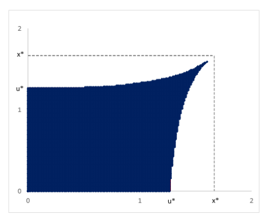
Figure 1: $E_{0}$ with $\lambda=3$, $a=0.7936$, $b=0.0891$, $s^{\prime}=1$

The numerically generated plot of $E_{0}$ shown in Figure 1 clearly illustrates the preceding result. This plot was generated by examining the behavior of solutions from initial points $(x_{0},y_{0})$ on a 200 by 200 partition grid. As expected from the adverse effect of inter-stage interaction with $b>0$, the extinction region is larger then when $b=0.$ However, not all initial pairs $(x_{0},y_{0})$ in the set $[0,x^{\ast})\times[0,x^{\ast}/s^{\prime})$ lead to extinction, a somewhat non-intuitive outcome.

4 Summary and open problems

In this paper, we established general results about the convergence to origin of orbits of the system (1)-(2) in the positive quadrant of the plane when $\lambda>1$. These extinction results that involve time-dependent parameters, are in line with expectations about the behavior of the orbits of the system.

We also studied the special case where $s_{n}=0$ for all $n$ in greater detail and determined that while the existence of fixed points in the positive quadrant is a sufficient condition for survival, it is not necessary. This surprising fact is true when $b>0,$ i.e. when the stages (adults and juveniles) interact within each period $n$ but false if $b=0$ and inter-stage interactions do not occur, a case that includes first-order population models where there are no stages or age-structuring. Also non-intuitively, we found that although the Allee equilibrium moves away from the origin due to interactions between stages and leads to an enlargement of the extinction region, this enlargement is not the maximum possible allowed by the shift.

There are many open questions about the nature of the extinction region $E$, and its complement, the survival region. We pose a few of these questions as open problems. The first concerns the base component $E_{0}$ of $E$.

Problem 15

Determine $E_{0}$ and its boundary, namely the extinction or Allee threshold, under the hypotheses of Corollary 13(c).

The numerically generated image in Figure 1 suggests that Problem 15 has a nontrivial solution. This problem naturally leads to the following.

Problem 16

Determine the extinction set $E$ under the hypotheses of Corollary 13(c).

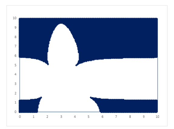
Figure 2: $E$ (shaded) and its complement for $\lambda=3$, $a=0.7936$, $b=0.0891$, $s^{\prime}=1$

Figure 2 illustrates a numerically generated part of $E$. This figure shows 3 distinct components, two of which are unbounded. The following result verifies that $E$ must have unbounded components.

Proposition 17

Assume that $\lambda>1$ and (24) holds. Let $u_{\ast}$ as defined in Lemma 6, be the point such that $f(u_{\ast})=u^{\ast}$. If

$$(x_{0},x_{1})\in R_{0,1}\cup R_{1,0}\cup R_{1,1}$$

where the rectangles $R_{0,1},R_{1,0},R_{1,1}$ are defined as

$$R_{0,1}=[0,u^{\ast})\times[u_{\ast},\infty),\quad R_{1,0}=[u_{\ast},\infty)\times[0,u^{\ast}),\quad R_{1,1}=[u_{\ast},\infty)\times[u_{\ast},\infty)$$

then corresponding orbits of (27) converge to zero, i.e. the above set is contained in the extinction region $E$.

Proof. For $i=0,1$, if $x_{i}<u^{\ast}$, then by Lemma 8, $\lim_{k\rightarrow\infty}x_{i+2k}=0$. If $x_{i}\geq u_{\ast}$, then

$$x_{i+2}=x_{i}^{\lambda}e^{a-bx_{i+1}-x_{i}}=f(x_{i})e^{-bx_{i+1}}\leq u^{\ast}e^{-bx_{i+1}}<u^{\ast}$$

and the rest is again a consequence of Lemma 8.   

We also saw that even when (27) has no positive fixed points if (33) holds, the set $E$ is not the entire quadrant $[0,\infty)^{2}$. This surprising fact is illustrated in the numerically generated panels in Figure 3. We also see in this figure that $E$ has fewer distinct components for the larger value of $b$ and that the survival region (unshaded) gets disconnected when the components of $E$ join.

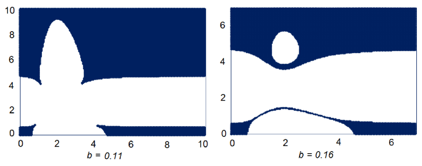
Figure 3: $E$ for $\lambda=2$, $a=1.1$, $s^{\prime}=1$ and two different values of $b$

These figures motivate the following.

Problem 18

Determine the extinction set $E$, or more to the point, its complement the survival set, when (33) holds.

Settling the following conjecture may be relevant to the preceding study.

Conjecture 19

Assume that (33) holds. Then for every positive solution $\{x_{n}\}$ of (27) at least one of the two subsequences $\{x_{2n}\}$ or $\{x_{2n-1}\}$ converges to zero.

Another direction to pursue involves extending the range of the parameter $a$.

Problem 20

Explore the extinction and survival regions if $a>\lambda-(\lambda-1)\ln\lambda$.

Finally, it may be appropriate to close with the following.

Problem 21

Extend the preceding analysis to the more general equation (11) with $s>0$ and $b>0.$

References

- [1] Ackleh, A.S. and Jang, S.R.-J., A discrete two-stage population model: continuous versus seasonal reproduction, J. Difference Eq. Appl. 13, 261-274, 2007
- [2] Allee, W. C., The Social Life of Animals, William Heinman, London, 1938.
- [3] Allee, W. C., Emerson, A.E., Park O., Park T., and Schmidt, K.P., Principles of Animal Ecology, WB Saunders, Philadelphia, 1949.
- [4] Berec, L., Angulo, E. and Courchamp, F., Multiple Allee effects and population management, TRENDS in Ecol. Evol., 22, 185-191, 2006.
- [5] Courchamp, F., Berec, L. and Gascoigne, J., Allee Effects in Ecology and Conservation, Oxford University Press, Oxford, 2008.
- [6] Cushing, J.M., Oscillations in age-structured population models with an Allee effect, J. Comput. Appl. Math., 52, 71-80, 1994.
- [7] Cushing, J.M., An Introduction to Structured Population Dynamics. CBMS-NSF Regional Conference Series in Applied Mathematics 71, SIAM, Philadelphia, 1998.
- [8] Cushing, J.M., A juvenile-adult model with periodic vital rates, J. Math Biol,, 53, 520-539, 2006.
- [9] Cushing, J.M., Backward bifurcations and strong Allee effects in matrix models for the dynamics of structured populations, J. Biol. Dyn., 8, 57-73, 2014.
- [10] Cushing, J.M. and Hudson, J.T., Evolutionary dynamics and strong Allee effects, J. Biol. Dyn., 6, 941-958, 2012.
- [11] Elaydi, S. N. and Sacker, R. J., Basin of attraction of periodic orbits of maps in the real line, J. Difference Eq. Appl., 10, 881-888, 2004.
- [12] Elaydi, S. N. and Sacker, R. J., Population models with Allee effects: A new model, J. Biol. Dyn., 4, 397-408, 2010.
- [13] Jang, Sophia R.-J., Allee effects in discrete-time host-parasitoid model, J. Difference Eq. Appl., 12, 165-181, 2006.
- [14] Lazaryan, N. and Sedaghat, H. Dynamics of planar systems that model stage-structured populations, Discr. Dyn. Nature Society, 2015, Article ID 137182, 2015. doi: 10.1155/2015/137182.
- [15] Lidicker, W.Z., The Allee effect: Its history and future importance, Open Ecol. J., 3, 71-82, 2010.
- [16] Livadiotis, G. and Elaydi, S., General Allee effect in two-species population biology, J. Biol. Dyn, 6, 959-973, 2014.
- [17] Liz, E., Pilarczyk, P., Global dynamics in a stage-sturctured discrete-time population model with harvesting, J. Theor. Biol. 297, 148-165, 2012.
- [18] Luis, R., Elaydi, S.N., and Oliveira, H., Non-autonomoous periodic systems with Allee effects, J. Difference Eq. Appl., 16, 1179-1196, 2010.
- [19] Schreiber, S.J., Allee effects, extinctions, and chaotic transients in simple population models, Theor. Popul. Biol., 64, 201-209, 2003.
- [20] Sedaghat, H., Folding, cycles and chaos in planar systems, J. Difference Eq. Appl., 21, 1-15, 2015.
- [21] Yakubu, A., Multiple attractors in juvenile-adult single species models, J. Difference Eq. Appl., 9, 1083-1098, 2007.
- [22] Zipkin, E.F., Kraft, C.E., Cooch, E.G., and Sullivan, P.J., When can efforts to control nuisance and invasive species backfire? Ecol. Appl. 19, 1585-1595, 2009.