Numerical methods for simulating the motion of porous balls in simple 3D shear flows under creeping conditions

Abstract

In this article, two novel numerical methods have been developed for simulating fluid/porous particle interactions in three-dimensional (3D) Stokes flow. The Brinkman-Debye-Bueche model is adopted for the fluid flow inside the porous particle, being coupled with the Stokes equations for the fluid flow outside the particle. The rotating motion of a porous ball and the interaction of two porous balls in bounded shear flows have been studied by these two new methods. The numerical results show that the porous particle permeability has a strong effect on the interaction of two porous balls.

Keywords Porous particles; Brinkman-Debye-Bueche model; Stokes flow, Particle suspension.

Classification: AMS: 65M60

1 Introduction

The study of interactions of fluid flow with porous particles is of great interest. Porous materials are everywhere. The skin, bones and a lot of organs of human body are porous. Daily foods like bread, vegetables and meats and building materials such as bricks, concrete and limestone are also porous. In medicine and biomedical engineering, biological membranes and filters provide other examples of porous materials. In electrochemical processes, permeable diaphragms and electrodes are further examples of porous materials. There are a lot of practical cases about flow around and through porous materials in industrial processes: A typical example concerns the production of paper from a pulp suspension; indeed, the flow of water around and through a pulp floc is a flow around and within a porous medium. In [1, 2, 3, 4, 5, 6, 7, 8, 9] there are studies of the porous contexts in agglomeration, chromatography, drug diliverly and tissue engineering, pulp and paper manufacturing and waste-water treatment. Darcy’s law [10] is the most common model of porous media flow studies and is a reliable formula as discussed in [11]. However, Darcy’s law has some limitations: For example, velocity gradients cannot be dealt with due to shear like those that occur at the boundary of the porous materials. Moreover, it is impossible for Darcy’s law to match the velocity and shear stress continuously for the interior and exterior flows at the particle surface since the Darcy’s law is a first order equation and Stokes equations, which govern the flow outside the porous particles, is second order. In order to solve the limitation on porous surface, Brinkman [12, 13] and Debue & Bueche [14] included the velocity gradient, which is not present in Darcy’s equation, and introduced the so-called Brinkman-Debye-Bueche (BDB) model. Since then, many theoretical studies have been focused on flow past rigid porous bodies, including [15, 16, 17, 18, 19, 20, 21] for single particle flow, and [22, 23, 24] for flow past two porous particles. It is important to understand the rheology of the suspension of porous particles in fluid flow, one major application being that porous particles can be used as carriers for drug delivery as, e.g., in [25, 26]. In [21], Masoud et al. studied numerically the influence of the permeability on the rotation rate of a porous ellipsoid in simple shear flows at the Stokes regime, based on the Brinkman-Debye-Bueche model. In [27], Li et al. studied the effect of the fluid inertia on the rotational behavior of a circular porous particle suspended in a two-dimensional simple shear flow. In this article, the Brinkman-Debye-Bueche model is adopted for the fluid flow inside the porous particle and then coupled with the Stokes equations for the fluid flow outside the particle. We have developed two novel numerical methods for simulating fluid/porous particle interactions in three-dimensions under creeping flow conditions. The rotation of a porous ball and the interaction of two porous balls in bounded shear flows have been studied. Numerical results show that, due to the permeability, two porous balls interact in bounded shear flows in a way quite different from that of two non-porous and rigid balls. The outline of this article is as follows: In Section 2, we will provide the system of equations modeling the fluid/porous particle interaction. Next, in Section 3 we will describe our numerical methods and present the results of the numerical simulation of the motion of one and then two porous balls in a bounded shear flow.

2 Governing equations

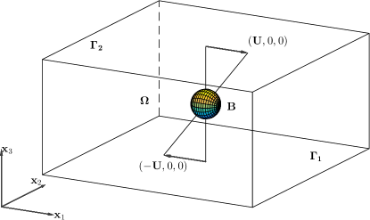
Figure 1: An example of a shear flow region with a porous ball $B$.

Without loss of generality, let us consider a neutrally buoyant and permeable ball $B$ moving in a bounded shear flow shown in Fig. 1 where $\Omega\subset\mbox{${\mathcal{R}}$}^{3}$ is a rectangular parallelepiped filled with a Newtonian viscous incompressible fluid. The flow governing equations outside the particle $B(t)$ are the following Stokes equations

$$\nabla\cdot\boldsymbol{\sigma}\equiv\nu\nabla^{2}\mathbf{u}-\nabla p={\bf 0}\text{ in }\Omega\setminus\overline{B(t)},\,\,t\in(0,T),$$ (1)

$$\nabla\cdot\mathbf{u}=0\text{ in }\Omega\setminus\overline{B(t)},\,\,t\in(0,T),$$ (2)

$${\bf u}={\bf g}_{0}\ \ {\rm on}\ \ \Gamma\times(0,T),\ {\rm with}\ \displaystyle\int_{\Gamma}{\bf g}_{0}\cdot{\bf n}\,d\Gamma=0,$$ (3)

where $\bf u$ is the flow velocity, $p$ is the pressure, $\nu$ is the fluid viscosity coefficient, $\Gamma$ is the union of the bottom boundary $\Gamma_{1}$ and top boundary $\Gamma_{2}$ as in Fig. 1, ${\bf n}$ is the unit normal vector pointing outward to the flow region, the boundary conditions being ${\bf g}_{0}=\{-U,0,0\}^{t}$ on $\Gamma_{1}$ and ${\bf g}_{0}=\{U,0,0\}^{t}$ on $\Gamma_{2}$ for a bounded shear flow. We assume also that the flow is periodic in the $x_{1}$ and $x_{2}$ directions with the periods $L_{1}$ and $L_{2}$, respectively.

According to the BDB model (e.g., see [21]), the fluid flow inside the porous particle is governed by the equations

$$\nabla\cdot\boldsymbol{\sigma}\equiv\nu\nabla^{2}\mathbf{u}-\nabla p=\nu k^{-1}(\mathbf{u}-\mathbf{u}_{p})\ \text{ in }B(t),\,\,t\in(0,T),$$ (4)

$$\nabla\cdot\mathbf{u}=0\ \text{ in }B(t),\,\,t\in(0,T),$$ (5)

where $k$ is the Darcy permeability and $\bf{u}_{p}$ is the velocity of the particle skeleton. The BDB and Stokes equations are coupled through the continuity of velocity and traction forces at the particle surface. The aforementioned governing equations for the fluid flow inside and outside of the porous particle have been considered in [21] for investigating the rotational speed of a porous particle of prolate ellipsoid shape in simple shear flows.

The motion of a neutrally buoyant ball satisfies the Euler-Newton’s equations:

$$\frac{d\mathbf{G}}{dt}=\mathbf{V},$$ (6)

$$M_{p}\frac{d\mathbf{V}}{dt}=\mathbf{F}_{H},$$ (7)

$${\mathbf{I}}_{p}\frac{d\boldsymbol{\omega}}{dt}=\mathbf{T}_{H},$$ (8)

$$\mathbf{G}(0)=\mathbf{G}_{0},\mathbf{V}(0)=\mathbf{V}_{0},\boldsymbol{\omega}(0)=\boldsymbol{\omega}_{0},$$ (9)

where $\mathbf{G}$ is the mass center of the porous particle, $M_{p}$ is the particle mass, $\mathbf{I}_{p}$ is the inertia tensor, ${\mathbf{V}}$ is the velocity of the mass center and $\boldsymbol{\omega}$ is the particle angular velocity. The motion $\mathbf{u}_{p}$ of the porous particle skeleton is given by

$$\mathbf{u}_{p}(\mathbf{x},t)=\mathbf{V}(t)+\boldsymbol{\omega}(t)\times\overrightarrow{\mathbf{Gx}},\forall{\mathbf{x}}\in\overline{B(t)},\,\,t\in(0,T).$$ (10)

For the hydrodynamical force and its resulting torque acting on the porous ball in (7) and (8), we have

$$\mathbf{F}_{H}=\int_{\partial B}\boldsymbol{\sigma}\mathbf{n}dS=\int_{B}\nabla\cdot\boldsymbol{\sigma}\,d\mathbf{x}=\nu k^{-1}\int_{B}(\mathbf{u}-\mathbf{u}_{p})\,d\mathbf{x},$$ (11)

$$\mathbf{T}_{H}=\int_{B}\overrightarrow{\mathbf{Gx}}\times(\nabla\cdot\boldsymbol{\sigma})d\mathbf{x}=\nu k^{-1}\int_{B}\overrightarrow{\mathbf{Gx}}\times(\mathbf{u}-\mathbf{u}_{p})d\mathbf{x},$$ (12)

where $\mathbf{n}=\{n_{1},n_{2},n_{3}\}^{t}$ is the unit normal vector pointing outward to the flow region.

The variational formulation for a porous particle freely moving in a Newtonian fluid under the creeping flow conditions is as follows: For a.e. $t>0$, find ${\mathbf{u}}(t)\in(H^{1}(\Omega))^{3},{\mathbf{u}}={\mathbf{g}}_{0}(t)$ on $\Gamma$, $p\in L^{2}_{0}(\Omega),\mathbf{G(t),V(t)},\boldsymbol{\omega(t)}\in\mathbb{R}^{3}$ such that

$$\nu\int_{\Omega}\nabla\mathbf{u}:\nabla\mathbf{v}\,d\mathbf{x}-\int_{\Omega}p\nabla\cdot\mathbf{v}\,d\mathbf{x}=-\frac{\nu}{k}\int_{B(t)}(\mathbf{u}-\mathbf{u}_{p})\cdot\mathbf{v}\,d\mathbf{x},\forall\mathbf{v}\in\mathbf{W}_{0},$$ (13)

$$\int_{\Omega}q\nabla\cdot\mathbf{u}\,d\mathbf{x}=0,\forall q\in L^{2}(\Omega),$$ (14)

$$\frac{d\mathbf{G}}{dt}=\mathbf{V},$$ (15)

$$M_{p}\frac{d\mathbf{V}}{dt}=\mathbf{F}_{H},$$ (16)

$${\mathbf{I}}_{p}\frac{d\boldsymbol{\omega}}{dt}=\mathbf{T}_{H},$$ (17)

$$\mathbf{G}(0)=\mathbf{G}_{0},\mathbf{V}(0)=\mathbf{V}_{0},\boldsymbol{\omega}(0)=\boldsymbol{\omega}_{0},$$ (18)

where in equations $(\ref{eqn:13})-(\ref{eqn:18})$, the function spaces are defined by

$$\mathbf{W}_{0}=\{\mathbf{v}\in(H^{1}(\Omega))^{3},\ \mathbf{v}|_{\Gamma}=\mathbf{0},\ \mathbf{v}\text{ is periodic in the }x_{1}\text{ and }x_{2}\text{ directions }$$

$$\hskip 40.0pt\text{with periods $L_{1}$ and $L_{2}$, respectively}\},$$

$$L^{2}_{0}(\Omega)=\{q|q\in L^{2}(\Omega),\int_{\Omega}q\,d\mathbf{x}=0\},$$

and

$$\mathbf{u}_{p}(\mathbf{x},t)=\mathbf{V}(t)+\boldsymbol{\omega}(t)\times\overrightarrow{\mathbf{G}(t)\mathbf{x}},\forall{\mathbf{x}}\in B(t),$$

$$\mathbf{F}_{H}=\frac{\nu}{k}\int_{B(t)}(\mathbf{u}-\mathbf{u}_{p})d\mathbf{x},$$

$$\mathbf{T}_{H}=\frac{\nu}{k}\int_{B(t)}\overrightarrow{\mathbf{G}(t)\mathbf{x}}\times(\mathbf{u}-\mathbf{u}_{p})d\mathbf{x}.$$

We have also modified formulation (13)-(18) for simulating one ball freely rotating and suspended initially at the middle between two moving walls in a bounded shear flow. To obtain the equilibrium rotational speed of such porous ball, we consider the following time dependent Stokes flow problem:

For $a.e.\quad t>0$, find ${\mathbf{u}}(t)\in(H^{1}(\Omega))^{3},{\mathbf{u}}={\mathbf{g}}_{0}(t)$ on $\Gamma$, $p\in L^{2}_{0}(\Omega),\mathbf{G(t),V(t)},\boldsymbol{\omega(t)}\in\mathbb{R}^{3}$ such that

$$\int_{\Omega}\frac{\partial\mathbf{u}}{\partial t}\cdot\mathbf{v}\,d\mathbf{x}+\nu\int_{\Omega}\nabla\mathbf{u}:\nabla\mathbf{v}\,d\mathbf{x}-\int_{\Omega}p\nabla\cdot\mathbf{v}\,d\mathbf{x}$$

$$\hskip 100.0pt=-\frac{\nu}{k}\int_{B(t)}(\mathbf{u}-\mathbf{u}_{p})\cdot\mathbf{v}\,d\mathbf{x},\forall\mathbf{v}\in\mathbf{W}_{0},$$ (19)

$$\int_{\Omega}q(\nabla\cdot\mathbf{u})\,d\mathbf{x}=0,\forall q\in L^{2}(\Omega),$$ (20)

$$\frac{d\mathbf{G}}{dt}=\mathbf{V}(t),$$ (21)

$$M_{p}\frac{d\mathbf{V}}{dt}=\mathbf{F}_{H},$$ (22)

$$\mathbf{I}_{p}\frac{d\boldsymbol{\omega}}{dt}=\mathbf{T}_{H},$$ (23)

$$\mathbf{u}(0)=\mathbf{u}_{0}\quad(\text{with}\nabla\cdot\mathbf{u}_{0}=0)\text{ in }\Omega,$$ (24)

$$\mathbf{G}(0)=\mathbf{G}_{0},\mathbf{V}(0)=\mathbf{V}_{0},\boldsymbol{\omega}(0)=\boldsymbol{\omega}_{0}.$$ (25)

In equation (24), $\mathbf{u}_{0}$ is the initial value of the velocity field $\mathbf{u}$.

3 Numerical methods and results

In this section, we like to present two novel numerical methodes for simulating the motion of porous balls in bounded shear flows based on the the coupled models discussed in Section 2. For the case of a single porous ball freely rotating and suspended initially at the middle between two moving walls, its mass center remains there. Its rotating speed with respect to the vorticity direction is a constant. To catch such a motion, we have to reach the steady state solution of equations (19)-(25); this can be done numerically. Similarly, to simulate the interaction of two porous balls in a bounded shear flow, we have to solve equations (13)-(18) numerically. Therefore we have developed in this section two different algorithms for simulating these two kinds of fluid/porous particle interaction. In this section, we assume that all dimensional quantities are in the CGS units.

3.1 Motion of a single porous ball

3.1.1 Description of the first numerical method

For the space discretization, we have used $P_{1}$-$iso$-$P_{2}$ and $P_{1}$ finite elements for the velocity field and pressure, respectively. More precisely, $h$ being the space discretization mesh size, we introduce a uniform tetrahedrization $\mathcal{T}_{h}$ and a twice coarser tetrahedrization $\mathcal{T}_{2h}$ of $\overline{\Omega}$. We approximate $(H^{1}(\Omega))^{3},\mathbf{W}_{0},L(\Omega)$ and $L^{2}_{0}(\Omega)$ by the following finite dimensional spaces

$$\mathbf{W}_{h}=\{\mathbf{v}_{h}|\mathbf{v}_{h}\in(C^{0}(\bar{\Omega}))^{3},\mathbf{v}_{h}|_{T}\in(P_{1})^{3},\forall T\in\mathcal{T}_{h},\mathbf{v}_{h}\text{ is periodic in the }x_{1}\text{ and }x_{2}$$

$$\hskip 40.0pt\text{directions with periods $L_{1}$ and $L_{2}$, respectively}\},$$

$$\mathbf{W}_{0,h}=\{\mathbf{v}_{h}|\mathbf{v}_{h}\in\mathbf{\mathbf{W}}_{h},\mathbf{v}_{h}=\mathbf{0}|_{\Gamma}\},$$

$$L^{2}_{h}=\{q_{h}|q_{h}\in C^{0}(\bar{\Omega}),q_{h}|_{T}\in P_{1},\forall T\in\mathcal{T}_{2h}\},$$

$$L^{2}_{0,h}=\{q_{h}|q_{h}\in L^{2}_{h},\int_{\Omega}q_{h}\,d\mathbf{x}=0\},$$

respectively; above, $P_{1}$ is the space of polynomials in three variables of degree $\leq 1.$

To simulate the motion of a single porous particle in a bounded shear flow, we look for a steady state of the rotation velocity field of the porous ball. To reach this steady state, we prefer working with formulation (19)-(25). Let $\Delta t$ be a time step and $t^{n}=n\Delta t$. The algorithm for solving the fully discrete analogue of system (19)-(25) reads as follows (after dropping some of subscripts $h$):

$\mathbf{u}^{0}=\mathbf{u}_{0}$, $\mathbf{G}^{0}=\mathbf{G}_{0}$, $\mathbf{V}^{0}=\mathbf{V}_{0}$, $\boldsymbol{\omega}^{0}=\boldsymbol{\omega}_{0}$, $\mathbf{u}_{p}^{0}=\mathbf{V}^{0}+\boldsymbol{\omega}^{0}\times\overrightarrow{\mathbf{G}^{0}\mathbf{x}}$ are known.

$\textit{For }n\geq 0,\mathbf{u}^{n},\mathbf{u}^{n}_{p},\mathbf{V}^{n},\mathbf{G}^{n}\textit{ and }\boldsymbol{\omega^{n}}\textit{being known, we solve the following sub-problems:}$

$\textit{Step 1. We compute }\mathbf{u}^{n+1}\textit{ and }p^{n+1}\textit{ via the solution of}$

$$\int_{\Omega}\frac{\mathbf{u}^{n+1}-\mathbf{u}^{n}}{\Delta t}\cdot\mathbf{v}\,d\mathbf{x}+\nu\int_{\Omega}\nabla\mathbf{u}^{n+1}:\nabla\mathbf{v}\,d\mathbf{x}-\int_{\Omega}p^{n+1}\nabla\cdot\mathbf{v}\,d\mathbf{x}$$

$$\hskip 100.0pt=-\frac{\nu}{k}\int_{B^{n}}(\mathbf{u}^{n}-\mathbf{u}^{n}_{p})\cdot\mathbf{v}\,d\mathbf{x},\forall\mathbf{v}\in\mathbf{W}_{0,h},$$ (26)

$$\int_{\Omega}q\nabla\cdot\mathbf{u}^{n+1}\,d\mathbf{x}=0,\forall q\in L^{2}_{h};$$ (27)

$$\mathbf{u}^{n+1}\in\mathbf{W}_{h},\mathbf{u}^{n+1}=\mathbf{g}_{0}(t^{n+1})\textit{ on }\Gamma,p^{n+1}\in L^{2}_{0,h}.$$

Step 2. Update the particle velocities and predict its mass center position:

$$M_{p}\frac{\mathbf{V}^{n+1}-\mathbf{V}^{n}}{\Delta t}=\frac{\nu}{k}\int_{B^{n}}(\mathbf{u}^{n+1}-\mathbf{u}^{n}_{p})d\mathbf{x},$$ (30)

$$\mathbf{I}_{p}\frac{\boldsymbol{\omega}^{n+1}-\boldsymbol{\omega}^{n}}{\Delta t}=\frac{\nu}{k}\int_{B^{n}}\overrightarrow{\mathbf{G}^{n}\mathbf{x}}\times(\mathbf{u}^{n+1}-\mathbf{u}_{p}^{n})\,d\mathbf{x},$$

$$\mathbf{G}^{n+1}=\mathbf{G}^{n}+\mathbf{V}^{n+1}\Delta t,$$

and then set (31)

$$\mathbf{u}^{n+1}_{p}=\mathbf{V}^{n+1}+\boldsymbol{\omega}^{n+1}\times\overrightarrow{\mathbf{G}^{n+1}x},\forall\mathbf{x}\in B^{n+1},$$

where $B^{n+1}$ is the new solid volume occupied by the porous ball centered at $\mathbf{G}^{n+1}$.

Remark 3.1

In equation (26), instead of having $\mathbf{u}^{n+1}$ in the right-hand side of the equation, we have used $\mathbf{u}^{n}$ there so that a fast solver can be applied to solve the linear systems at each iteration of an Uzawa/preconditioned conjugate gradient algorithm operating in the space $L^{2}_{0h}$ as discussed in, e.g., [28]. For the cases of a single porous ball suspended in a bounded shear flow, we want to obtain an equilibrium state, which is a spherical porous particle rotating at a constant speed at the middle between two moving planes. The stopping criterion for the steady state is set to be

$$\frac{1}{\Delta t}\|\mathbf{u}^{n+1}-\mathbf{u}^{n}\|<CRIT,$$

where CRIT is the tolerance. The numerical results obtained in the Section 3.1.2 have been obtaned with $CRIT=10^{-5}$.

Remark 3.2

When computing $\int_{B^{n}}(\mathbf{u}^{n}-\mathbf{u}^{n}_{p})\cdot\mathbf{v}\,d\mathbf{x}$ in equation (26), we have extended the integration to the entire computational domain $\Omega$ as follows

$$\int_{B^{n}}(\mathbf{u}^{n}-\mathbf{u}^{n}_{p})\cdot\mathbf{v}\,d\mathbf{x}=\int_{\Omega}{\chi}_{B^{n}}(\mathbf{u}^{n}-\mathbf{u}^{n}_{p})\cdot\mathbf{v}\,d\mathbf{x},$$

where $\chi_{B^{n}}$ is the characteristic function of the solid volume occupied by the ball centered at $\mathbf{G}^{n}$, i.e.,

$$\chi_{B^{n}}(\mathbf{x})=\begin{cases}1\quad\text{ if }\mathbf{x}\in B^{n},\\ 0\quad\text{ if }\mathbf{x}\notin B^{n}.\end{cases}$$

Then we have applied the trapezoidal rule on each tetrahedron in the tetrahedrization $\mathcal{T}_{h}$. To obtain the hydrodynamical forces and their resulting torques in equations (30) and (30), we have applied similar approaches.

Remark 3.3

For a rigid ball of radius $a$, the mass and inertia tensor are

$$M_{P}=\frac{4}{3}\pi a^{3}\ \rho_{s},$$

$$\mathbf{I}_{p}=\frac{2M_{P}}{5}\ a^{2}\begin{pmatrix}1&0&0\\ 0&1&0\\ 0&0&1\end{pmatrix},$$

where $\rho_{s}$ is the particle density. For a porous particle of the porosity $\tilde{P}$, we assume that the rigid skeleton is uniformly distributed over the entire volume of the porous ball so that its mass and inertia tensor are

$$M_{P}=\frac{4}{3}\pi a^{3}(\tilde{P}\rho_{f}+(1-\tilde{P})\rho_{s}),$$

$$\mathbf{I}_{P}=\frac{2M_{p}}{5}a^{2}\begin{pmatrix}1&0&0\\ 0&1&0\\ 0&0&1\end{pmatrix},$$

where $\rho_{f}$ is the fluid density. But for the neutrally buoyant ball considered in this article, the mass and inertia are the same as those of the rigid one since $\rho_{s}=\rho_{f}$.

3.1.2 Numerical results

Table 1: The rotational speed of the porous ball of radius $a=0.1$ obtained by $h=\frac{1}{48}$ and $CRIT=10^{-5}$

$\Delta t$	Permeability	$\omega(z)$
0.001	0.05	-0.4998402
0.001	0.01	-0.4999398
0.001	0.005	-0.4998876
0.001	0.0025	-0.4997966
0.001	0.001	-0.4996004
0.001	0.0005	-0.4994060
0.0005	0.00025	-0.4992049

Table 2: The rotational speed of the porous ball of radius $a=0.15$ obtained by $h=\frac{1}{48}$ and $CRIT=10^{-5}$

$\Delta t$	Permeability	$\omega$ (z)
0.001	0.05	-0.4998634
0.001	0.01	-0.4995757
0.001	0.005	-0.4992370
0.001	0.0025	-0.4987220
0.001	0.001	-0.4978223
0.001	0.0005	-0.4971082
0.0005	0.00025	-0.4964840

Table 3: The rotational speed of the porous ball of radius $a=0.2$ obtained by $h=\frac{1}{48}$ and $CRIT=10^{-5}$

$\Delta t$	Permeability	$\omega$ (z)
0.001	0.05	-0.4996081
0.001	0.01	-0.4983921
0.001	0.005	-0.4972581
0.001	0.0025	-0.4957328
0.001	0.001	-0.4934660
0.001	0.0005	-0.4919084
0.0005	0.00025	-0.4906672

(a) 

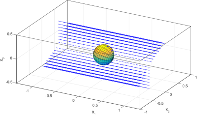
(b) 

(c) 

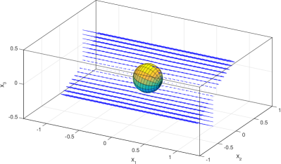
Figure 2: Snapshots of the velocity field projected on the shear plane ($x_{1}x_{3}$-plane) for a porous ball of radius $0.2$ rotating in a bounded shear flow: the values of the permeability are (a) $k=$0.05, (b) $k=$0.01, and (c) $k=$0.005, respectively (from top to bottom).

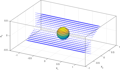
(d)  (e) 

(f) 

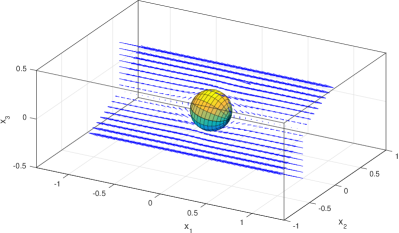
(g) 

Figure 3: Snapshots of the velocity field projected on the shear plane ($x_{1}x_{3}$-plane) for a porous ball of radius $0.2$ rotating in a bounded shear flow: the values of the permeability are (d) $k=$0.0025, (e) $k=$0.001, (f) $k=$0.0005 and (g) $k=$0.00025, respectively (from top to bottom).

We have considered the cases of one porous ball freely rotating and suspended initially at the middle between two moving walls as in Fig. 1. The computational domain is $\Omega=(-1,1)\times(-1/2,1/2)\times(-1,1)$. The radius of the ball is $a$=0.1, 0.15, or 0.2 and the initial position of the ball mass center is at $(0,0,0)$. The densities of the ball and fluid are both 1 and the fluid viscosity is also 1, thus the ball is neutrally buoyant. The values of the permeability $k$ of the porous ball considered here are 0.05, 0.01, 0.005, 0.0025, 0.001, 0.0005 and 0.00025. The shear rate for the shear flow is $\dot{\gamma}=1$. The space mesh size for the velocity field is $h=\frac{1}{48}$, the time step being $\Delta t=10^{-3}$. The rotating speed of a rigid ball in an unbounded shear flow is $-\dot{\gamma}/2$ according to the Jeffery’s solution [29]. For different values of the permeability and the radius of the ball, the rotating speed of a porous rigid ball in a bounded shear flow is in a good agreement with the Jeffery’s solution as shown in Tables 1, 2 and 3. The same conclusion has been obtained for the rotating speed of a porous ellipsoid in shear flows reported in [21]. But even if the rotating velocity inside the particle is the same as the rigid body motion, the fluid flow inside the porous ball does depend on the permeability. In Figs. 2 and 3, the projection of the velocity field on the $x_{1}x_{3}$-plane clearly indicates that the fluid motion is close to the rigid body motion only for much smaller value of the permeability (e.g., $k=$0.0005 and 0.00025). For the higher value of the permeability (e.g., $k=$0.05 and 0.01), the fluid just goes through the particle directly.

3.2 Motion of two porous balls

In this section we will consider numerical simulation of the interaction of two porous balls in a bounded shear flow. Due to that fact that these two porous balls can move freely between the two moving walls, we will employ (14)-(18) for simulating the dynamics of the two porous ball interaction.

3.2.1 Description of the second numerical method

The space-time discretization of (14)-(18) is presented in the following (again, after dropping some of subscripts $h$):

For $n\geq 0$, $\mathbf{u^{n},V_{i}^{n},G_{i}^{n}}$ and $\boldsymbol{\omega_{i}^{n}}$, $i=1$, $2$, being known (then $B^{n}_{i}$, $i=1,2$, are known), we solve the following sub-problems: Step 1. We compute $\mathbf{u^{n+1}}$, $p^{n+1}$, $\mathbf{V}_{i}^{n+1}$ and $\boldsymbol{\omega}_{i}^{n+1}$, $i=1$, $2$, via the solution of

$$\hskip-15.0pt\nu\int_{\Omega}\nabla\mathbf{u}^{n+1}:\nabla\mathbf{v}\,d\mathbf{x}-\int_{\Omega}p^{n+1}(\nabla\cdot\mathbf{v})\,d\mathbf{x}$$

$$\hskip 100.0pt=-\frac{\nu}{k}\sum_{i=1}^{2}\int_{B^{n}_{i}}(\mathbf{u}^{n+1}-\mathbf{u}^{n+1}_{p,i})\cdot\mathbf{v}\,d\mathbf{x},\ \forall\mathbf{v}\in\mathbf{W}_{0,h},$$ (32)

$$\hskip-15.0pt\int_{\Omega}q\nabla\cdot\mathbf{u}^{n+1}\,d\mathbf{x}=0,\ \forall q\in L^{2}_{h},$$ (33)

$$\hskip-15.0ptM_{p,i}\frac{\mathbf{V}_{i}^{n+1}-\mathbf{V}_{i}^{n}}{\Delta t}=\frac{\nu}{k}\int_{B^{n}_{i}}(\mathbf{u}^{n+1}-\mathbf{u}^{n+1}_{p,i})d\mathbf{x},\ i=1,2,$$ (34)

$$\hskip-15.0pt\mathbf{I}_{p,i}\frac{\boldsymbol{\omega}_{i}^{n+1}-\boldsymbol{\omega}_{i}^{n}}{\Delta t}=\frac{\nu}{k}\int_{B^{n}_{i}}\overrightarrow{\mathbf{G}_{i}^{n}\mathbf{x}}\times(\mathbf{u}^{n+1}-\mathbf{u}^{n+1}_{p,i})\,d\mathbf{x},\ i=1,2,$$ (35)

$$\hskip-15.0pt\mathbf{u}^{n+1}\in\mathbf{W}_{h},\mathbf{u}^{n+1}={\mathbf{g}}_{0}(t^{n+1})\textit{ on }\Gamma,\ p^{n+1}\in L^{2}_{0,h}.$$ (36)

Step 2. Update the particle mass centers:

$$\mathbf{G}_{i}^{n+1}=\mathbf{G}_{i}^{n}+\mathbf{V}_{i}^{n+1}\Delta t,\ i=1,2.$$ (37)

In (32)-(36), we have $\mathbf{u}^{n+1}_{p,i}(\mathbf{x})=\mathbf{V}_{i}^{n+1}+\boldsymbol{\omega}_{i}^{n+1}\times\overrightarrow{\mathbf{G}_{i}^{n}\mathbf{x}}$, $\forall\mathbf{x}\in B^{n}_{i}$ for $i=1,2$.

To solve problem (32)-(36), we consider it as a discrete analog of the following coupled system steady state:

For a.e. $t>0$, find $\mathbf{u}(t)\in(H^{1}(\Omega))^{3},\mathbf{u}={\mathbf{g}}_{0}$ on $\Gamma$, $p(t)\in L^{2}_{0}(\Omega)$, $\mathbf{V}_{i}$, $\boldsymbol{\omega}_{i}\in\mathbb{R}^{3}$, $i=1,2$, such that

$$\int_{\Omega}\frac{\partial\mathbf{u}}{\partial t}\cdot\mathbf{v}\,d\mathbf{x}+\nu\int_{\Omega}\nabla\mathbf{u}:\nabla\mathbf{v}\,d\mathbf{x}-\int_{\Omega}p\nabla\cdot\mathbf{v}dx$$

$$\hskip 100.0pt=-\frac{\nu}{k}\sum_{i=1}^{2}\int_{B_{i}}(\mathbf{u}-\mathbf{u}_{p,i})\cdot\mathbf{v}\,d\mathbf{x},\forall\mathbf{v}\in\mathbf{W}_{0},$$ (38)

$$\int_{\Omega}q(\nabla\cdot\mathbf{\mathbf{missing}}\mathbf{u})\,d\mathbf{x}=0,\forall q\in L^{2}(\Omega),$$ (39)

$$\mathbf{u}(0)=\mathbf{u}_{0}\text{ (with }\nabla\cdot\mathbf{u}_{0}=0)\text{ in }\Omega,$$ (40)

$$M_{p,i}(\mathbf{V}_{i}-\mathbf{V}_{0,i})=\frac{\nu\Delta t}{k}\int_{B_{i}}(\mathbf{u}-\mathbf{u}_{p,i})\,d\mathbf{x},\ i=1,2,$$ (41)

$$\mathbf{I}_{p,i}(\boldsymbol{\omega}_{i}-\boldsymbol{\omega}_{0,i})=\frac{\nu\Delta t}{k}\int_{B_{i}}\overrightarrow{\mathbf{G}_{i}^{n}\mathbf{x}}\times(\mathbf{u}-\mathbf{u}_{p,i})\,d\mathbf{x},\ i=1,2.$$ (42)

In system (38)-(42), we have $\mathbf{u}_{p,i}(\mathbf{x})=\mathbf{V}_{i}+\boldsymbol{\omega}_{i}\times\overrightarrow{\mathbf{G}_{i}^{n}\mathbf{x}}$, $\forall\mathbf{x}\in B_{i}$ for $i=1,2$, where the mass center $\mathbf{G}_{i}^{n}$ is fixed, $\mathbf{V}_{0,i}$ and $\boldsymbol{\omega}_{0,i}$ are given for $i=1,2$. Thus the region $B^{n}$ occupied by ball is fixed.

Combining the finite element approximations used in Section 3.1 with he backward Euler scheme we obtain the following discrete analogue of (38)-(42): $\mathbf{u}^{(0)}=\mathbf{u}^{n}$, $\mathbf{V}^{(0)}_{i}=\mathbf{V}_{i}^{n}$, $\boldsymbol{\omega}_{i}^{(0)}=\boldsymbol{\omega}_{i}^{n}$, $\mathbf{u}_{p,i}^{(0)}=\mathbf{V}_{i}^{(0)}+\boldsymbol{\omega}_{i}^{(0)}\times\overrightarrow{\mathbf{G}_{i}^{n}\mathbf{x}}$, $i=1,2$, are known.

For $m\geq 0$, $\mathbf{u^{(m)}}$, ${\mathbf{V}}_{i}^{(m)}$, $\boldsymbol{\omega}_{i}^{(m)}$, $\mathbf{u}^{(m)}_{p,i}$, $i=1,2$ being known, we solve the following sub-problems:

Step 1. We compute $\mathbf{u}^{(m+1)}\textit{ and }p^{(m+1)}$ via the solution of

$$\int_{\Omega}\frac{\mathbf{u}^{(m+1)}-\mathbf{u}^{(m)}}{\tau}\cdot\mathbf{v}\,d\mathbf{x}+\nu\int_{\Omega}\nabla\mathbf{u}^{(m+1)}:\nabla\mathbf{v}\,d\mathbf{x}-\int_{\Omega}p^{(m+1)}(\nabla\cdot\mathbf{v})\,d\mathbf{x}$$

$$\hskip 100.0pt=-\frac{\nu}{k}\sum_{i=1}^{2}\int_{B_{i}}(\mathbf{u}^{(m)}-\mathbf{u}^{(m)}_{p,i})\cdot\mathbf{v}\,d\mathbf{x},\quad\forall\mathbf{v}\in\mathbf{W}_{0,h},$$ (43)

$$\int_{\Omega}q\nabla\cdot\mathbf{\mathbf{missing}}u^{(m+1)}\,d\mathbf{x}=0,\forall q\in L^{2}_{h};$$ (44)

$$\mathbf{u}^{(m+1)}\in\mathbf{W}_{h},\mathbf{u}^{(m+1)}={\mathbf{g}}_{0}^{n+1}\textit{ on }\Gamma,\ p^{(m+1)}\in L^{2}_{0,h}.$$

Step 2. Update the values

$$M_{p,i}{\mathbf{V}_{i}^{(m+1)}-\mathbf{V}_{0,i}}=\frac{\nu{\Delta t}}{k}\int_{B_{i}}(\mathbf{u}^{(m+1)}-\mathbf{u}^{(m)}_{p,i})\,d\mathbf{x},\ i=1,2,$$ (45)

$$\mathbf{I}_{p,i}{\boldsymbol{\omega}_{i}^{(m+1)}-\boldsymbol{\omega}_{0,i}}=\frac{\nu{\Delta t}}{k}\int_{B^{n}_{i}}\overrightarrow{G_{i}^{n}\mathbf{x}}\times(\mathbf{u}^{(m+1)}-\mathbf{u}^{(m)}_{p,i})\,d\mathbf{x},\ i=1,2,$$ (46)

and set

$$\mathbf{u}_{p,i}^{(m+1)}=\mathbf{V}_{i}^{(m+1)}+\boldsymbol{\omega}_{i}^{(m+1)}\times\overrightarrow{\mathbf{G}_{i}^{n}\mathbf{x}},\quad\forall\mathbf{x}\in B_{i},\ i=1,2.$$ (47)

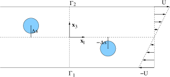
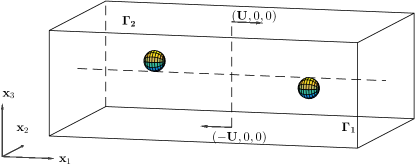
Figure 4: The initial position of two porous balls in a bounded shear flow region.

Remark 3.4

We have, again, used $\mathbf{u}^{(m)}$ in the right hand side of equation (43) so that a fast solver can be applied at each iteration when solving system (43)-(47) by an Uzawa/preconditioned conjugate gradient algorithm operating in the space $L^{2}_{0h}$ as discussed in, e.g., [28]. For the cases of two porous balls suspended in a bounded shear flow, where we are looking for a steady state solution, we stoped algorithm (43)-(47) as soon as

$$\frac{1}{\tau}\|\mathbf{u}^{(m+1)}-\mathbf{u}^{(m)}\|<CRIT,$$

where CRIT is the tolerance. The numerical results obtained in the Section 3.2.2 have been obtaned with $CRIT=10^{-5}$.

Remark 3.5

For the two ball interaction in a bounded shear flow, there is no lubrication force between the two balls under creeping flow conditions. Therefore, we are not allowed to apply an artificial repulsive force to prevent ball overlapping in numerical simulation since such force might alter the trajectories of the two ball mass centers. To deal with the interaction during the two ball interaction, we have to impose a minimal gap of size $ch$ between the balls where $c$ is some constant between 0 and 1, $h$ being the mesh size of the velocity field. Then, when advancing the two ball mass centers in equation (37), we proceed as follows at each sub-cycling time step: (i) we do nothing if the gap between the two balls at the new position is greater or equal than $ch$, (ii) if the gap size of the two balls at the new position is less than $ch$, we do not advance the balls directly; but instead we first move the ball centers in the direction perpendicularly to the line joining the previous centers, and then move them in the direction parallel to the line joining the previous centers, and make sure that the gap size is no less than $ch$.

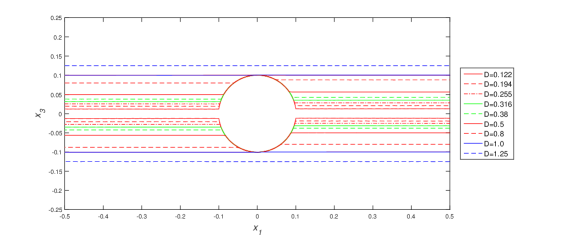
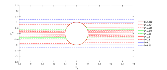
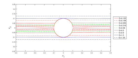
Figure 5: Trajectories of the ball mass centers in a bounded shear flow for the permeability $k=$0.05, 0.01, 0.005 and 0.0025 from top to bottom).

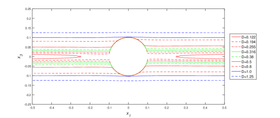
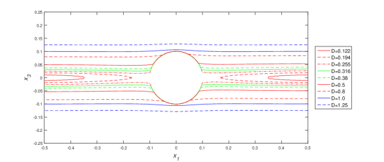
Figure 6: Trajectories of the ball mass centers in a bounded shear flow for the permeability $k=$0.001, 0.0005 and 0.00025 from top to bottom).

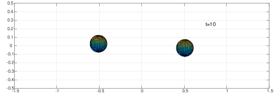
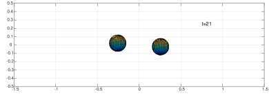
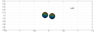
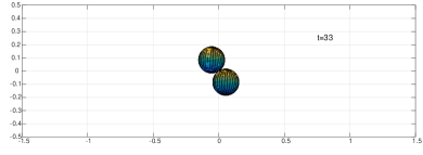
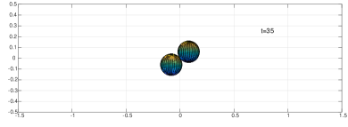
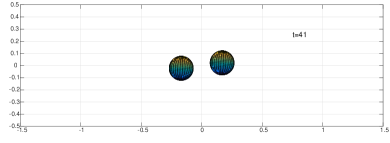
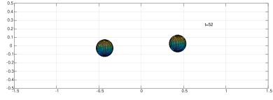
Figure 7: The snapshots of the particle position for the permeability $k=0.0005$ and $D=\Delta s/2a$=0.255 at $t=$10, 21, 28, 33, 35, 41, and 52 (from top to bottom and left to right).

3.2.2 Numerical results

We have considered the cases of two porous balls freely suspended initially on the $x_{1}x_{3}$-plane as in Fig. 4. The computational domain is $\Omega=(-1.5,1.5)\times(-1/2,1/2)\times(-1,1)$. The two ball radii are $a=$ 0.1. The initial position of the two ball mass centers are at $(-0.75,0,\triangle s)$ and $(0.75,0,-\triangle s)$ for a given vertical displacement $\triangle s>0$ (see Fig. 4). The values of the vertical displacement are $D=\Delta s/2a=$0.122, 0.194, 0.255, 0.316, 0.38, 0.5, 0.8, 1.0 and 1.255. The densities of the ball and fluid are both 1 and the fluid viscosity is also 1. Thus the balls are neutrally buoyant. The values of the permeability $k$ of the porous ball are 0.05, 0.01, 0.005, 0.0025, 0.001, 0.0005 and 0.00025. The shear rate for the shear flow is 1. The space mesh size for the velocity field is $h=\frac{1}{48}$. The time step is $\Delta t=0.001$ for $k=$0.05, 0.01, 0.005, 0.0025, 0.001, and 0.0005 and $\Delta t=0.0005$ for $k=$0.00025.

In the Stokes regime, the interaction of the two non-porous and rigid balls in simple shear flows has been well studied (see, e.g., [30]). Zurita et al. obtained that, depending of their vertical initial height $\triangle s$, the balls pass over/under each other or rotate around the midpoint of their mass centers if they are located as in Fig. 4 initially. The first kind is called the non-swapping of the trajectories of the two ball mass centers, i.e., the higher one takes over the lower one and then both return to their initial heights while moving in a bounded shear flow. The second kind is called the swapping of the trajectories, i.e., they come close to each other and to the mid-plane between the two horizontal walls, then, the balls move away from each other and from the above mid-plane. For those wondering about the influence of porosity on the ball interaction let us mention the following: For the higher values of the permeability (e.g., $k=$ 0.05, 0.01, 0.005 and 0.0025), the two porous balls pass over/under each other for the vertical displacements as in Fig. 5. Also for the cases of smaller values of $k$ in Fig. 6, the two porous balls still have non-swapping trajectories for most values of the vertical displacement. For these non-swapping between two porous balls, the two balls first come toward to each other, then almost touch each other and rotate with respect to the midpoint between two ball mass centers, and finally separate (see Fig. 7 for the details). Thus, the interaction of the two non-swapping porous balls is quite different from the one between two non-porous and rigid balls as reported in [30]. When viewing the vector field in Figs. 2 and 3, it is not surprising to see that the streamlines go through the porous ball, which explain why we have obtained such kind of non-swapping trajectories for the two porous balls. But for the lower permeability cases, the swapping between two porous balls are obtained for smaller values of the vertical displacement (e.g., $\Delta s/2a$=0.122 for $k=$ 0.001 and 0.005 and $\Delta s/2a$=0.122 and 0.184 for $k=$0.00025).

References

• [1] P. Vainshtein and M. Shapiro, Porous agglomerates in the general linear flow field, J. Colloid Interface Sci., 298 (2006), pp. 183-191.
• [2] M. Vanni and A. Gastaldi, Hydrodynamic forces and critical stresses in low-density aggregates under shear flow, Langmuir, 27 (2011), pp. 12822-12833.
• [3] W. M. Deen, Hindered transport of large molecules in liquid-filled pores, AIChE J. 33 (1987), pp. 1409-1425.
• [4] F. E. Regnier, Perfusion chromatography, Nature, 350 (1991), pp. 634-635.
• [5] M. A. C. Stuart,W. T. S. Huck, J. Genzer, M. Muller, C. Ober, M. Stamm, G. B. Sukhorukov, I. Szleifer, V. V. Tsukruk, M. Urban, F. Winnik, S. Zauscher, I. Luzinov, and S. Minko, Emerging applications of stimuli-responsive polymer materials, Nat. Mater., 9 (2010), pp. 101-113.
• [6] H. Masoud and A. Alexeev, Controlled release of nanoparticles and macromolecules from responsive microgel capsules, ACS Nano, 6 (2010), pp. 212-219.
• [7] H. Masoud, B. I. Bingham, and A. Alexeev, A.Designing maneuverable micro-swimmers actuated by responsive gel, Soft Matt., 8 (2012), pp. 8944-8951.
• [8] M. Deng and C. T. J. Dodson, Random star patterns and paper formation, Tappi J., 77 (1994), pp. 195-199.
• [9] W. Gujer and M. Boller, Basis for the design of alternative chemical-biological waste-water treatment processes, Prog. Water Technol., 10 (1978), pp. 741-758.
• [10] H. Darcy, Les Fontaines Publiques de la Ville de Dijon: Exposition et Application, Victor Dalmont, 1856.
• [11] S. Whitaker, Flow in porous media: a theoretical derivation of Darcy’s law, Transport in Porous Media, 1 (1986), pp. 3-13.
• [12] H. C. Brinkman, A calculation of the viscous force exerted by a flowing fluid on a dense swarm of particles, Appl. Sci. Res., A1 (1947), pp. 7-34.
• [13] H. C. Brinkman, On the permeability of media consisting of closely packed porous particles swarm of particles, Appl. Sci. Res., A1 (1947), pp. 81-86.
• [14] P. Debye and A. M. Bueche, Intrinsic viscosity, diffusion, and sedimentation rate of polymers in solution, J. Chem. Phys., 16 (1948), pp. 573-579.
• [15] P. M. Adler and P. M. Mills, Motion and rupture of a porous ball in a linear flow field, J. Rheol., 23 (1979), pp. 25-37.
• [16] T. Zlatanovski, Axisymmetric creeping flow past a porous prolate spheroidal particle using the Brinkman model, Q. J. Mech. Appl. Math., 52 (1999), pp. 111-126.
• [17] J. P. Hsu and Y. H. Hsieh, Drag force on a porous, non-homogeneous spheroidal floc in a uniform flow field, J. Colloid Interface Sci., 259 (2003), pp. 301-308.
• [18] P. Vainshtein, M. Shapiro, and C. Gutfinger, Mobility of permeable aggregates: effects of shape and porosity, J. Aerosol Sci., 35 (2004), pp. 383-404.
• [19] B. Cichocki and B. U. Felderhof, Hydrodynamic friction coefficients of coated spherical particles, J. Chem. Phys., 130 (2009), 164712.
• [20] S. T. T. Ollila, T. Ala-Nissila, and C. Denniston, Hydrodynamic forces on steady and oscillating porous particles, J. Fluid Mech., 709 (2012), pp. 123-148.
• [21] H. Masoud, H. A. Stone and M. J. Shelley, On the rotation of porous ellipsoids in simple shear flows, J. Fluid Mech., 733 (2013), R6.
• [22] P. Reuland, B. U. Felderhof, and R. B. Jones, Hydrodynamic interaction of two spherically symmetric polymers, Physica A, 93 (1978), pp. 465-475.
• [23] H. Yano, A. Kieda, and I. Mizuno, The fundamental solution of Brinkman equation in 2 dimensions, Fluid Dyn. Res., 7 (1991), pp. 109-118.
• [24] J. Richardson and H. Power, A boundary element analysis of creeping flow past two porous bodies of arbitrary shape, Engng. Anal. Bound. Elem., 17 (1996), pp. 193-204.
• [25] E. Tasciotti, X. Liu, R. Bhavane, K. Plant, A. D. Leonard, B. K. Price, M. M. C. Cheng, P. Decuzzi, J. M. Tour, F. Robertson, and M. Ferrari, Mesoporous silicon particles as a multistage delivery system for imaging and therapeutic applications, Nature Nanotechnology, 3 (2008), pp. 151-157.
• [26] S. Zhang, K. Kawakami, L. K. Shrestha, G. C. Jayakumar, J. P. Hill, and K. Ariga, Totally Phospholipidic Mesoporous Particles, J. Phys. Chem. C, 119 (2015), pp. 7255-7263.
• [27] C. Li, M. Ye, and Z. Liu, On the rotation of a circular porous particle in 2D simple shear flow with fluid inertia, J. Fluid Mech., 808 (2016), R3.
• [28] R. Glowinski, Finite element methods for incompressible viscous flows, in: Handbook of Numerical Analysis (P. G. Ciarlet and J. L. Lions, eds.), vol. IX, North-Holland, Amsterdam, 2003, pp. 3-1176.
• [29] G. B. Jeffery, The motion of ellipsoidal particles immersed in a viscous fluid, Proc. R. Soc. Lond. A, 102 (1922), pp. 161-79.
• [30] M. Zurita-Gotor, J. Blawzdziewicz, and E. Wajnryb, Swapping trajectories: a new wall-induced mechanism in a dilute suspension of spheres, J. Fluid Mech., 592 (2007), pp. 447-469.