Sparse Approximation is Provably Hard under Coherent Dictionaries

Abstract

It is well known that sparse approximation problem is NP-hard under general dictionaries. Several algorithms have been devised and analyzed in the past decade under various assumptions on the coherence $\mu$ of the dictionary represented by an $M\times N$ matrix from which a subset of $k$ column vectors is selected. All these results assume $\mu=O(k^{-1})$. This article is an attempt to bridge the big gap between the negative result of NP-hardness under general dictionaries and the positive results under this restrictive assumption. In particular, it suggests that the aforementioned assumption might be asymptotically the best one can make to arrive at any efficient algorithmic result under well-known conjectures of complexity theory. In establishing the results, we make use of a new simple multilayered PCP which is tailored to give a matrix with small coherence combined with our reduction.

1 Introduction

Given a dictionary $\Phi$ with normalized columns, represented by an $M\times N$ matrix ($\Phi\in\mathbb{R}^{M\times N}$) and a target signal $y\in\mathbb{R}^{M}$ such that the columns of $\Phi$ span $\mathbb{R}^{M}$, sparse approximation problem asks to find an approximate representation of $y$ using a linear combination of at most $k$ atoms, i.e. column vectors of $\Phi$. This amounts to finding a coefficient vector $x\in\mathbb{R}^{N}$ for which one usually solves

$$\min_{{\|x\|}_{0}=k}{\|y-\Phi x\|}_{2}$$ (1)

We name the problem with this standard objective function (1) as Sparse. Stated in linear algebraic terms, it is essentially about picking a $k$-dimensional subspace defined by $k$ column vectors of $\Phi$ such that the orthogonal projection of $y$ onto that subspace is as close as possible to $y$. The reader should note that the problem can be defined with full generality using notions from functional analysis (e.g. Hilbert spaces with elements representing functions), as is usually conceived in signal processing. Indeed, defined in Hilbert and Banach spaces, it has been studied as highly nonlinear approximation in functional approximation theory [20, 21]. However, we consider linear algebraic language as any kind of generalization is irrelevant to our discussion and the negative results we will present can be readily extended to the general case.

Although mainly studied in signal processing and approximation theory, sparse approximation problem is of combinatorial nature in finite dimensions and the optimal solution can be found by checking all $\binom{N}{k}$ subspaces. It is natural to ask whether one can do better and the answer partly lies in the fact that Sparse is NP-hard even to approximate within any factor [8, 18] under general dictionaries. The intrinsic difficulty of the problem under this objective function prevents one from designing algorithms which can even approximate the optimal solution. Hence, efforts have been towards analyzing algorithms working on a restricted set of dictionaries for which one requires the column vectors to be an almost orthogonal set, namely an incoherent dictionary. Formally, one defines the coherence $\mu$ of a dictionary $\Phi$ as

$$\mu(\Phi)=\max_{i\neq j}|\langle\Phi_{i},\Phi_{j}\rangle|$$

where $\Phi_{i}$ and $\Phi_{j}$ are the $i^{th}$ and $j^{th}$ columns of $\Phi$, respectively and $\langle\cdot,\cdot\rangle$ denotes the usual inner product defined on $\mathbb{R}^{M}$. Recall that the columns of a dictionary have unit norm. Hence, the coherence $\mu$ takes values in the $[0,1]$ closed interval.

There are roughly three types of algorithmic results regarding sparse approximation problem as listed below.

1. Results relating the quality of the solution ${\|y-\Phi x\|}_{2}$ produced by the algorithm to the quality of the optimal solution ${\|y-\Phi x^{*}\|}_{2}$ given that $\mu(\Phi)$ is a slowly growing or decreasing function of $k$.

2. Results showing the rate of convergence of an algorithm for elements from a specific set related to the dictionary (e.g. [15])

3. Results stating conditions under which an algorithm optimally recovers a signal either via norms of certain matrices related to the dictionary (e.g. [23]) or the Restricted Isometry Property (RIP) (e.g. [7]).

The results of this paper are immediately related to the first kind, which are expressed via Lebesgue-type inequalities as named by Donoho et al. [9]. Accordingly, we shall define the following:

Definition 1.1.

An algorithm is an $(f(k),g(k))$-approximation algorithm for Sparse under coherence $h(k)$ if it selects a vector $x$ with at most $g(k)$ nonzero elements from the dictionary $\Phi$ with $\mu(\Phi)\leq h(k)$ such that

$$\|y-\Phi x\|_{2}\leq f(k)\cdot\|y-\Phi x^{*}\|_{2}$$

where $x^{*}$ is the optimal solution with at most $k$ nonzero elements.

Orthogonal Matching Pursuit (OMP) is a well studied greedy algorithm yielding such approximation guarantees. There is also a slight variant of this algorithm named Orthogonal Least Squares (OLS). In the last decade, the following results were found in a series of papers by different authors:

Theorem 1.2.

[11] OMP is an $(8\sqrt{k},k)$-approximation algorithm for Sparse under coherence $\frac{1}{8\sqrt{2}(k+1)}$.

Theorem 1.3.

[23] OMP is a $(\sqrt{1+6k},k)$-approximation algorithm for Sparse under coherence $\frac{1}{3k}$.

Theorem 1.4.

[9] OMP is a $(24,\lfloor k\log{k}\rfloor)$-approximation algorithm for Sparse under coherence $\frac{1}{90k^{3/2}}$.

Theorem 1.5.

[22] OMP is a $(3,2^{\lfloor\frac{1}{\delta}\rfloor}k)$-approximation algorithm for Sparse under coherence $\frac{1}{14\left(2^{\lfloor\frac{1}{\delta}\rfloor}k\right)^{1+\delta}}$, for any fixed $\delta>0$.

Theorem 1.6.

[16] OLS is a $(3,2k)$-approximation algorithm for Sparse under coherence $\frac{1}{20k}$.

In this paper, we are particularly interested in an approximation of the form $(f(k),k)$ which implies a solution to the standard sparse approximation problem. We will investigate the possibility of such an approximation with respect to $h(k)$. First, let us discuss these algorithmic results qualitatively. First, notice that all the results assume a coherence of $O(k^{-1})$. Indeed, it is a curious question whether such a restrictive assumption is needed for approximating the problem. There is no trivial answer. Another peculiarity is that all the results are essentially due to OMP (or a slight variant), which is a simple and intuitive greedy algorithm reminiscent of the greedy method for the well known Set Cover problem in combinatorial optimization. This method is optimal due to a result of Feige [10] with respect to approximating the best solution. In essence, sparse approximation can also be considered as a covering problem where we want to cover a target vector using vectors from a given set. Of course, unlike Set Cover which does not bear any contextual information on the elements, one also needs to take the linear algebraic content into account. Hence, thinking in purely analogical manner, one would expect that OMP is probably the best algorithm one can hope for under the definition of approximation we have provided and the assumption of $\mu=O(k^{-1})$ is most likely necessary. Although our results are not exactly tight and there is still some room for improvement (algorithmic and/or complexity theoretic), as we will see, this intuition is correct to a certain extent.

We would like to note that intuitive reasonings about why one might need coherence have already been discussed in the literature. The question whether one needs coherence is explicitly articulated in [4] where it is pointed out that “for if two columns are closely correlated, it will be impossible in general to distinguish whether the energy in the signal comes from one or the other”. However strong this intuition is, there is no complexity theoretic barrier for solving the sparse approximation problem under reasonably coherent dictionaries. There naturally arises the question of how much coherence makes the problem intractable. For instance, does there exist a polynomial time algorithm for sparse approximation under some very small constant or inverse logarithmic coherence? This is the conceptual issue we address in this paper. This work can also be seen as a continuation of our effort to prove hardness results using the standard PCP tools for problems of linear algebraic nature. The rationale of the constructions of the current paper are similar to the ones in our previous results where we prove hardness results for subset selection problems in matrices [5, 6].

1.1 Main Results

We prove the following two theorems, which state the hardness of Sparse under coherence as a function of $k$ (the number of atoms to be selected):

Theorem 1.7.

For any constant $\epsilon>0$, and any function $f$, there is a sparsity parameter $k$ such that there is no polynomial time $(f(k),k)$-approximation algorithm for Sparse under coherence $\epsilon$ unless P = NP.

Theorem 1.8.

For any constants $c>0$ and $\epsilon>0$, there is a sparsity parameter $k$ such that there is no polynomial time $(c,k)$-approximation algorithm for Sparse under coherence $k^{-1+\epsilon}$ unless Unique Games is in P.

Both theorems are the result of the same reduction with different PCPs. Note that the first theorem rules out all sorts of approximation. This is due to the fact that we have perfect completeness in the PCP which implies $\|y-\Phi x\|=0$ in the YES case of our reduction. Our construction ensures that this value is strictly greater than $0$ for the NO case implying that there is no approximation at all under the assumption P $\neq$ NP. As for the second theorem, Unique Games is a problem proposed and conjectured to be NP-hard by Khot [13], the so called Unique Games Conjecture (UGC). Even though the assumption of the theorem is known to be stronger than the famous P $\neq$ NP, current algorithmic techniques fall short of proving Unique Games to be in P. In fact, there are many strong inapproximability results assuming UGC. A famous example is the Max-Cut problem for which a tight hardness result was proven by Khot et al. [14]. Since the PCP implied by the UGC does not have perfect completeness, it will be the case that $\|y-\Phi x\|=\epsilon$ for some small positive $\epsilon$ in the YES case of our reduction. In the NO case, we will have some explicit constant value for $\|y-\Phi x\|$, thereby ruling out a constant factor approximation only, unlike the strong result in the first theorem.

We would like to underline that our reductions do not imply any hardness results for compressed sensing. The dictionaries we construct are very special deterministic matrices which do not seem to be of any use in this field. We only make sure that the column vectors of the dictionary span the whole space which is the standard assumption in sparse approximation. In fact, it is an interesting challenge to come up with complexity theoretic barriers for compressed sensing, say parameterized with the restricted isometry constant. Such investigations however, are beyond the scope of this paper.

2 Motivation: The Two Layered PCP

As is usual in most hardness results, our starting point is the PCP theorem [2, 3] combined with Raz’s parallel repetition theorem [19]. In this section, we define the constraint satisfaction problem implied by these two theorems and prove a preliminary result showing the hardness of sparse approximation under coherence $1/2+\epsilon$. The constraint satisfaction problem that we will make use of should satisfy an extra property called “smoothness”, which is usually not implied by the PCP theorem together with Raz’s parallel repetition theorem. However, we find it convenient to state the usual construction first, and then point out its deficiencies and why we need smoothness. This will also allow the reader to follow the main reasoning of our actual reduction and why the Unique Games Conjecture is involved in the second theorem. We then prove our main theorems using multilayered PCPs in the next two sections.

The constraint satisfaction problem of our interest is often called the Label Cover problem, first introduced in [1]. A Label Cover instance $L$ is defined as follows: $L=(G(V,W,E),\Sigma_{V},\Sigma_{W},\Pi)$ where

• $G(V,W,E)$ is a regular bipartite graph with vertex sets $V$ and $W$, and the edge set $E$.

• $\Sigma_{V}$ and $\Sigma_{W}$ are the label sets associated with $V$ and $W$, respectively.

• $\Pi$ is the collection of constraints on the edge set, where the constraint on an edge $e$ is defined as a function $\Pi_{e}\colon\Sigma_{V}\rightarrow\Sigma_{W}$.

The problem is to satisfy as many constraints as possible by finding an assignment $A\colon V\rightarrow\Sigma_{V}$, $A\colon W\rightarrow\Sigma_{W}$. A constraint $\Pi_{e}$ is said to be satisfied if $\Pi_{e}(A(v))=A(w)$ where $e=(v,w)$. Starting from a MAX3-SAT instance in which each variable occurs exactly $5$ times, one can define a (fairly well known) reduction to the Label Cover problem. Applying what is called a parallel repetition to the instance at hand, one can then get a new Label Cover instance $L$ for which $|V|=(5n/3)^{u}$, $|W|=n^{u}$, $|E|=(5n)^{u}$, $|\Sigma_{V}|=7^{u}$, $|\Sigma_{W}|=2^{u}$, the degree of the vertices in $V$ is $d_{V}=3^{u}$, and the degree of the vertices in $W$ is $d_{W}=5^{u}$, where $n$ is the number of variables in the MAX3-SAT instance and $u$ is the number of parallel repetitions. The following is a standard result.

Theorem 2.1.

(PCP theorem [2, 3] and Raz’s parallel repetition theorem [19]) Let $L$ be given as above. There exists a universal constant $\gamma>0$ such that for every large enough constant $u$, it is NP-hard to distinguish between the following two cases:

• YES. There is an assignment $A\colon V\rightarrow\Sigma_{V}$, $A\colon W\rightarrow\Sigma_{W}$ such that $\Pi_{e}$ is satisfied for all $e\in E$.

• NO. No assignment can satisfy more than a fraction $2^{-\gamma u}$ of the constraints in $\Pi$.

The idea of our reduction is simple. The vector $y$ we want to approximate is composed of all $1$s. In the YES case, we want to ensure that there are $k$ column vectors in $\Phi$ whose linear combinations can “cover” all the coordinates of $y$. In the NO case, we want to have that there are no $k$ column vectors that can cover all the coordinates. Hence, consider the following reduction from Label Cover to Sparse inspired by a well known reduction proving hardness for the Set Cover problem [17]: We first define a set of vectors $x_{1},x_{2},\ldots,x_{2^{u}}$ consisting of only $0$s and $1$s, and then normalize them. The set also satisfies the property that the dot product of any two vectors in it is $1/2$. It is not difficult to construct such a vector set; the rows of a Hadamard matrix of size $2^{u+1}$ readily provides one. Specifically, in all reductions we present from now on, we consider a Hadamard matrix of size $2^{x+1}$ where we need at most $2^{x}$ distinct codewords covering half of the coordinates. This is by the fact that one of the rows of the Hadamard matrix is all $1$s and should be discarded. Thus, the remaining $2^{x+1}-1>2^{x}$ rows suffice for our purpose. Given $L$ as above, we define $2^{u}$ column vectors for each $w\in W$, one for each label in $\Sigma_{W}$. Let the column vectors defined for $w$ be $\Phi_{w,1},\ldots,\Phi_{w,2^{u}}$. These column vectors have $(5n)^{u}$ disjoint blocks, one for each edge in $E$. For each $e\in E$ which is incident to $w\in W$, the block of $\Phi_{w,i}$ corresponding to $e$ consists of a specified vector, say $x_{i}$. The blocks of $\Phi_{w,i}$ corresponding to the edges which are not incident to $w$ are all zeros. Finally, we normalize $\Phi_{w,i}$ so that it has norm $1$ and set $k=|V|+|W|=(5n/3)^{u}+n^{u}$.

The reduction performs a similar operation to the left hand side of the bipartite graph. The usual practice in covering type problems is to define on $V$, the complement of the vectors on $W$ in accordance with the projection function $\Pi$ of $L$, where taking a complement of a vector in this context means inverting its $0$s and $1$s. We refer the reader to Figure 1 and Figure 2 for an illustration of the column vectors defined corresponding to a simple Label-Cover instance where the complement of a vector $x$ is denoted by $\overline{x}$. Here, there are $|E|=(5n)^{u}$ blocks in each column vector where each block is given by a specific Hadamard code. Thus, the number of coordinates of a single column vector is $M=2^{u+1}(5n)^{u}$. This construction ensures that in the YES case of $L$ where there is a labeling satisfying all the edges, one can prove the existence of a subset of column vectors complementing each other on all the coordinates, thereby “covering” the target vector $y$. However, there arises the following typical problem due to the fact that the label sizes $|\Sigma_{V}|=7^{u}$ and $|\Sigma_{W}|=2^{u}$ are not equal: In order to make sure that the main idea of the reduction works, one is also inherently forced to define a total of $2^{u}$ distinct vectors for a given $v\in V$, just as we did for the vertices in $W$. But, there are $7^{u}$ labels in $\Sigma_{V}$. This may result in more than one copies of the same column vector meaning that the coherence of the dictionary may be very large, in particular $1$, since there is no restriction on how the projection function $\Pi$ distributes $7^{u}$ labels in $\Sigma_{V}$ to $2^{u}$ labels in $\Sigma_{W}$. (Note that in this case, we have that the total number of columns $N=7^{u}|V|+2^{u}|W|=(35n/3)^{u}+(2n)^{u}$). This is the key point where our reduction deviates from the usual Set Cover type reductions. In order to ensure a small coherence, we need a more intricate structure or a stronger assumption. Accordingly, Theorem 1.7 is proved using what is called a Smooth Label Cover instance and Theorem 1.8 is proved using the Unique Label Cover instance which appears in the definition of the Unique Games Conjecture. To be complete, there is one technicality that must be handled: The column vectors of $\Phi$ must span $\mathbb{R}^{M}$. This can easily be satisfied by adding the identity matrix of size $M\times M$ to the set of all column vectors.

We now give a theorem stating the existence of a two layered Smooth Label Cover instance from [12].

Theorem 2.2 ([12]).

Given a Label Cover instance $L=(G(V,W,E),\Sigma_{V},\Sigma_{W},\Pi)$ with $|\Sigma_{V}|=7^{(T+1)u}$ and $|\Sigma_{W}|=2^{u}7^{Tu}$, there is an absolute constant $\gamma>0$ such that for all integer parameters $u$ and $T$, it is NP-hard to distinguish between the following two cases:

• YES. There is an assignment $A\colon V\rightarrow\Sigma_{V}$, $A\colon W\rightarrow\Sigma_{W}$ such that $\Pi_{e}$ is satisfied for all $e\in E$.

• NO. No assignment can satisfy more than a fraction $2^{-\gamma u}$ of the constraints in $\Pi$.

Furthermore, $L$ has the following “smoothness property”. For every $v\in V$, and $a_{1},a_{2}\in\Sigma_{V}$ such that $a_{1}\neq a_{2}$, if $w$ is a randomly chosen neighbor of $v$, then

$$Pr_{w}\left[\Pi_{(v,w)}(a_{1})=\Pi_{(v,w)}(a_{2})\right]\leq\frac{1}{T}.$$

One can further assume that $|V|=O(n^{Tu})$, $|W|=O(n^{Tu})$ and $G(V,W,E)$ is a regular bipartite graph where the degree of the vertices in $V$ is $d_{V}={(T+1)u\choose u}3^{u}$ and the degree of the vertices in $W$ is $d_{W}=5^{u}$.

Given the Smooth Label Cover instance whose existence is guaranteed by the theorem above, our reduction is similar to the one we described for the Label Cover instance. The vector $y$ we want to approximate is an all $1$s vector. In order to define $\Phi$, let $x_{1},x_{2},\ldots,x_{2^{u}7^{Tu}}$ be a set of vectors consisting of only $0$s and $1$s. Perform a normalization on these vectors, i.e. $x_{i}\leftarrow x_{i}/\|x_{i}\|_{2}$. Note that a coordinate of $x_{i}$ is either $0$ or a constant depending on $u$ and $T$, say $\eta$. We also have that the dot product of any two vectors in this set is $1/2$. As noted earlier, the rows of a Hadamard matrix of size $2^{u+1}7^{Tu}$ (which is a constant) satisfy this property. Given $L$ as above, we define $2^{u}7^{Tu}$ column vectors for each $w\in W$, one for each label in $\Sigma_{W}$. Let the column vectors defined for $w\in W$ be $\Phi_{w,1},\ldots,\Phi_{w,2^{u}7^{Tu}}$. These column vectors have $|E|=O(n^{Tu})$ disjoint blocks, one for each edge in $E$. For each $e\in E$ which is incident to $w\in W$, the block of $\Phi_{w,i}$ corresponding to $e$ consists of a specified vector $x_{i}$. The blocks of $\Phi_{w,i}$ corresponding to the edges which are not incident to $w$ are all zeros. Finally, we normalize $\Phi_{w,i}$ so that it has norm $1$.

Similar to $W$, we define a column vector for each vertex-label pair on $V$. Specifically, let $\overline{x_{i}}$ be the vector such that its $j$th coordinate $\overline{x_{ij}}=0$ if the $j$th coordinate $x_{ij}$ of $x_{i}$ is $\eta$, and $\overline{x_{ij}}=\eta$ if $x_{ij}=0$. Let the column vectors defined for $v\in V$ be $\Phi_{v,1},\ldots,\Phi_{v,7^{(T+1)u}}$. These column vectors have $|E|=O(n^{Tu})$ disjoint blocks, one for each edge in $E$. For each $e\in E$ which is incident to $v\in V$, the block of $\Phi_{v,i}$ corresponding to $e$ is the vector $\overline{x_{\Pi_{e}(i)}}$. The blocks of $\Phi_{v,i}$ corresponding to the edges which are not incident to $v$ are all zeros. We normalize $\Phi_{v,i}$ so that it has norm $1$ and set $k=|V|+|W|=O(n^{Tu})$. We finally add an identity matrix of size $M\times M$ to $\Phi$ in order to make sure that its column vectors span $\mathbb{R}^{M}$. As for the size of the reduction where we have $\Phi\in\mathbb{R}^{M\times N}$ and $y\in\mathbb{R}^{M}$, it is clear that $M=2^{u+1}7^{Tu}|E|=2^{u+1}7^{Tu}5^{u}|W|$ and $N=7^{(T+1)u}|V|+2^{u}7^{Tu}|W|$, which are both of polynomial size for $T$ and $u$ constant since $|V|$ and $|W|$ are both $O(n^{Tu})$. The mechanics of the reduction is best explained pictorially. For this reason, In Figure 1, we show a small part of a Smooth Label Cover instance. The corresponding matrix $\Phi^{T}$ is given in Figure 2.

We now prove the completeness of the reduction. Suppose that there is an assignment of the vertices in $V$ and $W$ which satisfies all the edges in $E$. Given such an assignment, take the corresponding column vectors of $\Phi$, a total of $k=|V|+|W|$ vectors. By the reduction, given a block corresponding to a specific edge $e=(v,w)$, we have that the column vectors selected from $v$ and $w$ cover all the coordinates allocated to $e$, i.e. the nonzero values in $v$ and $w$ complement each other. Thus, the selected $k$ column vectors cover all the $M$ coordinates and there exists a vector $x\in\mathbb{R}^{N}$ with $k$ nonzero entries satisfying $\Phi x=y$.

Suppose now that there is no assignment of the vertices that satisfies all the edges. First, note that in order to cover all the $M$ coordinates, one needs to select exactly $1$ column vector from each vertex in $V$ and $W$. Because, if there is a vertex $v$ from which no column vector is selected, one cannot cover the blocks of edges incident to $v$ by selecting one vector from the neighbors of $v$ (The rows of a Hadamard matrix cover only half of the coordinates). Hence, one needs to select multiple vectors to cover these blocks and it follows that all the coordinates cannot be covered by selecting $k$ column vectors. But, even if one selects $1$ vector from each vertex, the unsatisfied edges cannot be covered by the definition of the reduction. Hence, for all $x\in\mathbb{R}^{N}$, we have $\|y-\Phi x\|_{2}>0$. This shows that Sparse cannot be approximated at all given the conditions of $\Phi$ provided by our reduction.

It remains to see what the coherence of $\Phi$ is. First, note that the dot product of any two column vectors belonging to different vertices in $V$ or $W$ is $0$ since they do not share any blocks. Besides, the dot product between a column vector in $V$ and another column vector in $W$ is clearly (much) less than $1/2$ since they share at most one block. There remain two basic cases to check. The column vectors defined for a vertex $w\in W$ have half of their coordinates overlap with each other and hence all the pairs have dot product $1/2$. The situation is a little more involved for a vertex $v\in V$. Given $\Phi_{v,i}$ and $\Phi_{v,j}$, by the smoothness property of the Label Cover instance, we have that $\overline{x_{\Pi_{e}(i)}}=\overline{x_{\Pi_{e}(j)}}$ for at most $1/T$ fraction of the edges that are incident to $v$. Thus, the extra contribution we have for the dot product of two column vectors defined for $v$, because of having the same entries on some of the blocks, is at most $1/T$ (Note that, this is not satisfied by the usual Label Cover instance). It follows that the maximum dot product of any two column vectors of $\Phi$ is at most $1/2+1/T$. Hence, Sparse is NP-hard under dictionaries with coherence $1/2+\epsilon$ for arbitrarily small constant $\epsilon$ upon selecting $T$ arbitrarily large.

Figure 1: A part of a simple bipartite graph representing a Smooth Label Cover instance

Figure 2: The resulting (row) vectors in Sparse instance computed from the graph in Figure 1 by our reduction

3 Reduction from the Multilayered Smooth Label Cover

(a) The two layered PCP

(b) The corresponding multilayered PCP that we make use of

Figure 3:

In this section, we define a simple multilayered PCP starting from a two layered Smooth Label Cover instance. Let $L=(G(V,W,E),\Sigma_{V},\Sigma_{W},\Pi)$ be such a Label Cover instance defined as in the previous section. An $\ell$-layered Smooth Label Cover instance $L^{\ell}$ is defined as follows: $L^{\ell}=(G^{\ell}(X_{1},\ldots,X_{\ell},E^{\ell}),\Sigma_{V},\Sigma_{W},\Pi^{\ell})$ where $\ell$ is an even positive integer and

• $G^{\ell}(X_{1},\ldots,X_{\ell},E^{\ell})$ is a multipartite hyper-graph with vertex sets $X_{1},X_{2},\ldots,X_{\ell}$ and the hyper-edge set $E$.

• $X_{i}=V$ for odd $i$, and $X_{i}=W$ for even $i$, where $1\leq i\leq\ell$.

• $E^{\ell}$ consists of all hyper-edges of the form $(v,w,v,w,\ldots,v,w)$ on $\ell$ vertices belonging to $X_{1},\ldots,X_{\ell}$, respectively where $v\in V$, $w\in W$ and $(v,w)\in E$.

• $\Pi^{\ell}$ is the collection of constraints on the hyper-edge set, where the constraint on a hyper-edge $e=(x_{1},x_{2},\ldots,x_{\ell-1},x_{\ell})=(v,w,\ldots,v,w)$ is itself defined as a collection of $\ell-1$ constraints of the form $\Pi_{(x_{2i-1},x_{2i})}\colon\Sigma_{V}\rightarrow\Sigma_{W}$ for $i=1,\ldots,\ell/2$, and $\Pi_{(x_{2i+1},x_{2i})}\colon\Sigma_{V}\rightarrow\Sigma_{W}$ for $i=1,\ldots,\ell/2-1$, where $x_{i}\in X_{i}$ for $i=1,\ldots,\ell$, and all the constraints are identical to $\Pi_{(v,w)}$.

As usual, one is asked to find an assignment for all the vertices of the instance, i.e. construct functions $A_{2i-1}\colon X_{i}\rightarrow\Sigma_{V}$, and $A_{2i}\colon X_{i}\rightarrow\Sigma_{W}$ for $i=1,\ldots,\ell/2$, where the goal is to satisfy as many hyper-edges as possible. In this case however, there are two definitions of satisfiability. A constraint $\Pi_{e}$ is said to be strongly satisfied if all of the $\ell-1$ constraints defined for $e$ are satisfied. Otherwise, it is said to be weakly satisfied if only a fraction of its constraints are satisfied. This is the standard terminology introduced in Feige’s paper about the Set Cover problem [10] and the difference between strong and weak satisfiability is important in that context. However, we will be only arguing about the strong satisfiability in this work as it is sufficient to derive our hardness results.

The foregoing definition already defines a fairly straightforward reduction from the Smooth Label Cover instance to the multilayered instance: Just replace each layer alternatively by $V$ and $W$, define a hyper-edge in $e\in E^{\ell}$ for each edge $e^{\prime}=(v,w)\in E$ such that it contains all the copies of $v$ and $w$ in alternating layers (i.e. $e^{\prime}$ uniquely defines $e$), and finally define all the $\ell-1$ projection functions of a hyper-edge $e$ to be the projection function $\Pi_{e^{\prime}}$ on the corresponding edge $e^{\prime}$ of the original instance. The reduction is shown in Figure 3 where each hyper-edge of the multilayered instance is defined on exactly $\ell$ vertices, three of them straight, one zigzagging. Given this reduction, it is not difficult to see that if there is an assignment for $L$ which satisfies all the constraints, then the same assignment strongly satisfies all the constraints of $L^{\ell}$. Similarly, if no assignment satisfies more than a fraction $2^{-\gamma u}$ of the constraints in $L$, then no assignment strongly satisfies more than a fraction $2^{-\gamma u}$ of the constraints in $L^{\ell}$.

The rows of a Hadamard matrix was sufficient to give a set of vectors with pairwise dot products $1/2$. In order to get a coherence of arbitrarily small constant value starting from the $\ell$-layered instance defined above, we need a more general construction. The construction which we describe below is essentially inspired by that of partition systems mentioned by Feige [10]. However, it is not clear whether these systems satisfy conditions on the coherence that we require. They are tailored to prove hardness for Set Cover. Hence, we describe our construction from the first principles. This will also allow the reader to see why the construction works at an intuitive level. To this aim, we define an incoherent vector system $V(\ell,d)$. It has the following properties:

1. It is a set $V(\ell,d)$ of $\ell d$ normalized vectors of dimension $\ell^{d}$ with exactly $\ell^{d-1}$ nonzero coordinates of the same positive value.

2. $V(\ell,d)=\bigcup_{i=1}^{d}V(i,\ell,d)$ where $V(i,\ell,d)$ is a set of $\ell$ vectors for $i=1,\ldots,d$, and $V(i,\ell,d)\cap V(j,\ell,d)=\emptyset$ for $i\neq j$.

3. Any two distinct vectors in $V(i,\ell,d)$ have dot product $0$ for $i=1,\ldots,d$. Furthermore, the indices of the nonzero coordinates of the vectors in $V(i,\ell,d)$ cover the set $\{1,\ldots,\ell^{d}\}$.

4. For a vector $x\in V(i,\ell,d)$ and $y\in V(j,\ell,d)$, the dot product of $x$ and $y$ is $1/\ell$, where $i\neq j$.

For explicitly denoting vectors in the system, we let

$$V(i,\ell,d)=\{V_{1}(i,\ell,d),V_{2}(i,\ell,d),\ldots,V_{\ell}(i,\ell,d)\},$$

where the vectors are ordered lexicographically with respect to the nonzero entries in their coordinates. The result of the reduction of this section is provided by the following lemma.

Lemma 3.1.

There exists an explicit deterministic construction of an incoherent vector system $V(\ell,d)$ for all $1\leq d\leq\ell$.

Proof.

We will construct the desired vectors by describing a recursive procedure. Consider first the $\ell$ strings of length $\ell$ each with a distinct coordinate being $1$ and all other coordinates $0$ (e.g. for $\ell=3$, the strings are $100,010$ and $001$). Let these “seed” strings be $u_{1},u_{2},\ldots u_{\ell}$ in lexicographic order. For each of these strings, concatenate $\ell^{d-1}$ of them side by side to form $\ell$ strings of length exactly $\ell^{d}$. To give a better idea of the procedure, we will get the following strings for $\ell=d=3$:

$$v_{1}=100100100100100100100100100$$

$$v_{2}=010010010010010010010010010$$

$$v_{3}=001001001001001001001001001$$

Normalizing these $\ell$ strings, i.e. multiplying each coordinate by $\ell^{(1-d)/2}$ we obtain the vectors

$$V_{1}(d,\ell,d),V_{2}(d,\ell,d),\ldots,V_{\ell}(d,\ell,d),$$

which form the set $V(d,\ell,d)$. This makes a total of $\ell$ vectors of the incoherent vector system at the lowest level of our recursion. Note also that these vectors have pairwise dot product $0$.

In order to construct the vectors of $V(d-1,\ell,d)$, we create a set of new strings by “expanding” each coordinate of the seed string $u_{i}$, namely by repeating their coordinates exactly $\ell$ times in place. Thus, we get a new set of $\ell$ strings of length $\ell^{2}$ (e.g. for $\ell=3$, the aforementioned strings are $111000000,000111000$ and $000000111$). For each of these strings, concatenating $\ell^{d-2}$ of them side by side, we get $\ell$ strings of length $\ell^{d}$. Normalizing these strings, we obtain the vectors of the set $V(d-1,\ell,d)$. Note that the pairwise dot products of the vectors in this set are also $0$. Furthermore, the dot product of a vector in $V(d-1,\ell,d)$ and another vector in $V(d,\ell,d)$ is exactly $1/\ell$ as there are $\ell^{d-2}$ common nonzero coordinates between two such vectors and the nonzero entries are all $\ell^{(1-d)/2}$.

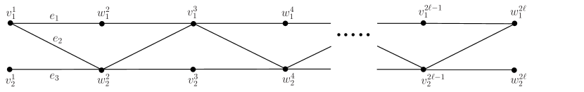
Figure 4: A part of a simple bipartite graph representing a multilayered Smooth Label Cover instance

Figure 5: Some of the resulting (row) vectors in Sparse instance computed from the graph in Figure 4 by our reduction

We repeat this procedure by constructing $\ell$ vectors in the upper level at each step until we finally construct the set $V(1,\ell,d)$. Specifically, for $1\leq k\leq d$ at step $k$, we expand the seed strings that are used in the previous step to get $\ell$ new seed strings of length $\ell^{k}$. Concatenating $\ell^{d-k}$ of these and normalizing the coordinates, we get the set of vectors $V(d-k+1,\ell,d)$. It is clear that the pairwise dot products in such a set are all $0$. Looking at two vectors $u\in V(i,\ell,d)$ and $v\in V(j,\ell,d)$ for $i\neq j$, we also have that their dot product is exactly $1/\ell$ since by construction they have $\ell^{d-2}$ common nonzero coordinates and each nonzero coordinate is $\ell^{(1-d)/2}$. Hence, we have $\ell d$ vectors in total forming the set $V(\ell,d)$ and all the properties of an incoherent vector system are satisfied. ∎

We are ready to describe our reduction. Given the Smooth Label Cover instance $L$, the derived multilayered instance $L^{\ell}$ and an incoherent vector system $V(\ell,d)$ as described above, we first construct $d=2^{u}7^{Tu}$ column vectors for each $w\in X_{2j}$ for $j=1,\ldots,\ell/2$. Specifically, given $w\in X_{2j}$, we define a vector for each one of the $d$ labels, namely the set:

$$\{V_{2j}(1,\ell,d),V_{2j}(2,\ell,d),\ldots,V_{2j}(d,\ell,d)\}.$$

Note that the dot products of any two of these vectors is $1/\ell$. Similar to the reduction presented in the previous section, the actual column vectors of the matrix $\Phi$ are composed of $|E^{\ell}|$ blocks, one for each hyper-edge (Note that $|E^{\ell}|=|E|=O(n^{Tu})$). The column vector $\Phi_{w,i}$ for $1\leq i\leq d$ is defined as follows: The blocks of the vector which correspond to the hyper-edges that contain $w$ is $V_{2j}(i,\ell,d)$ and all the other blocks consist of zeros. This reduction is in fact very similar to the one described for the two-layered Label Cover problem. Figure 4 is an example of a simple instance of a multilayered Label Cover problem, and Figure 5 illustrates the overall structure of the matrix produced by the reduction. For simplicity, we only show the vectors that belong to the vertices of the first four layers.

The column vectors of the odd layers of the instance $L^{\ell}$ are also defined similar to the previous section. Given $v\in X_{2j-1}$ where $1\leq j\leq\ell/2$, $\Phi_{v,i}$ consists of $|E^{\ell}|$ blocks for $i=1,\ldots 7^{(T+1)u}$. The block of $\Phi_{v,i}$ corresponding to hyper-edge $e\in E^{\ell}$ is $V_{2j-1}(\Pi_{e^{\prime}}(i),\ell,d)$ where $e^{\prime}\in E$ is the edge that uniquely determines $e$ and $\Pi$ is the projection function of $L$. We define $y$ to be the vector of all $1$s and $k=\sum_{i=1}^{\ell}|X_{i}|=\frac{\ell}{2}(|V|+|W|)$. We let $u$ and $T$ be constants and $\ell\gg d=2^{u}7^{Tu}$ be a constant. As usual, we extend $\Phi$ with an identity matrix of appropriate size so as to satisfy the condition of the sparse approximation problem. Note that the size of the reduction is polynomial. In particular, $M=\ell^{d}|E|=\ell^{2^{u}7^{Tu}}5^{u}|W|=O(n^{Tu})$ and $N=\frac{\ell}{2}(7^{(T+1)u}|V|+2^{u}7^{Tu}|W|)=O(n^{Tu})$ since $u,T,\ell$ are all constants, and $|V|$ and $|W|$ are both $O(n^{Tu})$.

Proof of Theorem 1.7:

• Completeness: Suppose that there is an assignment which satisfies all the edges of $L$. Consider the same assignment on $L^{\ell}$ on all layers, repeated $\ell/2$ times. As noted before, this assignment also strongly satisfies all the hyper-edges of $L^{\ell}$. Selecting all the $k$ column vectors defined by this assignment, we see that the coordinates of a block reserved for a hyper-edge $e=(x_{1},x_{2},\ldots,x_{\ell})$ can be covered by the column vectors corresponding to the labels assigned to $x_{1},x_{2},\ldots,x_{\ell}$. Because, they form a set

  $$\{V_{1}(\Pi_{e^{\prime}}(i),\ell,d),V_{2}(j,\ell,d),\ldots,V_{\ell-1}(\Pi_{e^{\prime}}(i),\ell,d),V_{\ell}(j,\ell,d)\},$$

  where $e^{\prime}\in E$ is the edge defining $e$, $\Pi_{e^{\prime}}$ is the constraint on $e^{\prime}$ and $i,j$ are the labels assigned to the vertices on alternate layers. But, $\Pi_{e^{\prime}}(i)=j$ since $e$ is strongly satisfied. Hence, by the definition of the incoherent vector system, we have that the aforementioned set exactly covers the coordinates corresponding to $e$. Since this is true for all the hyper-edges, the selected $k$ columns can cover all the $M$ coordinates. In other words there is a vector $x\in\mathbb{R}^{N}$ with $k$ nonzero entries such that $\Phi x=y$.

• Soundness: Suppose that no assignment satisfies more than a fraction $2^{-\gamma u}$ of the edges of $L$. Then, as noted before, no assignment strongly satisfies more than a fraction $2^{-\gamma u}$ of the hyper-edges in $L^{\ell}$. Our argument is similar to that of the two layered case. First, in order to cover all the $M$ coordinates, one needs to select exactly $1$ column vector from each vertex in all the layers. Because, if there is a vertex $v$ from which no column vector is selected, one cannot cover the blocks of hyper-edges incident to $v$ by selecting one vector from each neighbor of $v$ (The coordinates reserved for the layer that $v$ belongs to will never be completely covered). Hence, one needs to select multiple vectors to cover these blocks and it follows that all the coordinates cannot be covered by selecting only $k$ column vectors. It follows that it is sufficient to analyze the case where one selects exactly $1$ column vector from each vertex in the graph. In this case however, if there is a hyper-edge which is not strongly satisfied, by definition of the incoherent vector system, the block corresponding to that edge cannot be covered. Hence, for all choices of $x\in\mathbb{R}^{N}$, we have that $\|y-\Phi x\|_{2}>0$.

It remains to see what the coherence of $\Phi$ is. Similar to the two layered case, the dot product of two column vectors from distinct vertices in a layer is $0$, and the dot product of two column vectors belonging to different layers is smaller than $1/\ell$. Consider now the column vectors defined for the vertices in layers of even index. They are analogous to $W$ in the two layered case; there are $2^{u}7^{Tu}$ of them for one vertex, and any two column vectors corresponding to distinct labels have dot product $1/\ell$ by construction. The same construction goes through for the layers of odd index. However, there are $7^{(T+1)u}$ column vectors for one vertex and hence there are duplicates. Each constraint of a hyper-edge consists of $\ell-1$ constraints of the two layered instance. Recalling that hyper-edges in $E^{\ell}$ are in one to one correspondence the edges in $E$ and that the smoothness property is satisfied for $L$, we conclude that the amount of dot product coming from any two column vectors corresponding to $a_{1},a_{2}\in\Sigma_{V}$ such that $a_{1}\neq a_{2}$ is at most $1/T$. Thus, the coherence of the dictionary is upper bounded by $1/T+1/\ell$. Recalling that $\ell\gg d=2^{u}7^{Tu}$, the dominating term in this expression is $1/T$. By choosing $T$ arbitrarily large, it follows that Sparse is NP-hard under dictionaries with coherence $\epsilon$ for arbitrarily small $\epsilon>0$. $\blacksquare$

4 Reduction from the Multilayered Unique Label Cover

The main hindrance that prevents us from pushing the coherence below a constant is the term $1/T$. No matter how large a function we assign to $\ell$, the coherence remains at $1/T$ due to the construction. Ideally, one would like to avoid possible duplications of vectors in the odd layers of the multilayered instance, thereby completely getting rid of $1/T$ and selecting $\ell$ as large as possible. This is precisely what the constraint satisfaction problem mentioned in the famous Unique Games Conjecture provides. A Unique Label Cover instance $L$ is defined as follows: $L=(G(V,W,E),R,\Pi)$ where

• $G(V,W,E)$ is a regular bipartite graph with vertex sets $V$ and $W$, and the edge set $E$.

• $\Sigma=\{1,2,\ldots,R\}$ is the label sets associated with both $V$ and $W$.

• $\Pi$ is the collection of constraints on the edge set, where the constraint on an edge $e$ is defined as a bijective function $\Pi_{e}\colon\Sigma\rightarrow\Sigma$.

As usual, in the problem associated with a given instance, the goal is to satisfy as many constraints as possible by finding an assignment $A\colon V\rightarrow\Sigma$, $A\colon W\rightarrow\Sigma$. The following is the well-known conjecture by Khot [13]:

Conjecture 4.1.

(Unique Games Conjecture [13]) Let $L$ be defined as above. Given $\epsilon,\delta>0$, there exists a constant $R(\epsilon,\delta)$ such that it is NP-hard to distinguish between the following two cases:

• YES. There is an assignment $A\colon V\rightarrow\Sigma$, $A\colon W\rightarrow\Sigma$ such that at least $(1-\epsilon)$ fraction of the constraints in $\Pi$ are satisfied.

• NO. No assignment can satisfy more than a fraction $\delta$ of the constraints in $\Pi$.

It is possible that the conjecture is false, but the problem Unique Games is still not in P. In fact, this is the version stated in Theorem 1.8. We rule out the existence of a polynomial time algorithm for Sparse under certain conditions given that the problem described above is not in P.

Given a Unique Label Cover instance $L$, one can define an $\ell$-layered Unique Label Cover instance as follows (This is in same spirit to the one defined in previous section, see Figure 3): $L^{\ell}=(G^{\ell}(X_{1},\ldots,X_{\ell},E^{\ell}),R,\Pi^{\ell})$ where $\ell$ is an even positive integer and

• $G^{\ell}(X_{1},\ldots,X_{\ell},E^{\ell})$ is a multipartite hyper-graph with vertex sets $X_{1},X_{2},\ldots,X_{\ell}$ and the hyper-edge set $E$.

• $X_{i}=V$ for odd $i$, and $X_{i}=W$ for even $i$, where $1\leq i\leq\ell$.

• $E^{\ell}$ consists of all hyper-edges of the form $(v,w,v,w,\ldots,v,w)$ on $\ell$ vertices belonging to $X_{1},\ldots,X_{\ell}$, respectively where $v\in V$, $w\in W$ and $(v,w)\in E$.

• $\Pi^{\ell}$ is the collection of constraints on the hyper-edge set, where the constraint on a hyper-edge $e=(x_{1},x_{2},\ldots,x_{\ell-1},x_{\ell})=(v,w,\ldots,v,w)$ is itself defined as a collection of $\ell-1$ constraints of the form $\Pi_{(x_{2i-1},x_{2i})}\colon\Sigma\rightarrow\Sigma$ for $i=1,\ldots,\ell/2$, and $\Pi_{(x_{2i+1},x_{2i})}\colon\Sigma\rightarrow\Sigma$ for $i=1,\ldots,\ell/2-1$, where $x_{i}\in X_{i}$ for $i=1,\ldots,\ell$, and all the constraints are identical to $\Pi_{(v,w)}$.

As usual, one is asked to find an assignment for all the vertices of the instance, i.e. construct functions $A_{i}\colon X_{i}\rightarrow\Sigma$ for $i=1,\ldots,\ell$, where the goal is to satisfy as many hyper-edges as possible. A constraint $\Pi_{e}$ is said to be strongly satisfied if all of the $\ell-1$ constraints defined for $e$ are satisfied. The reduction from $L$ to $L^{\ell}$ is also quite straightforward and is in the same spirit as the one described in the previous section. Again, it is important here to see that each hyper-edge in $E^{\ell}$ is uniquely determined by an edge in $E$. Given the reduction, if there is an assignment for $L$ which satisfies at least $(1-\epsilon)$ fraction of the constraints, then the same assignment satisfies the set of hyper-edges that are uniquely determined by the satisfied edges in $L$, i.e. at least $(1-\epsilon)$ of the constraints in $L^{\ell}$ are strongly satisfied. It is also easy to see that if no assignment satisfies more than a fraction $\delta$ of the constraints in $L$, then no assignment strongly satisfies more than a fraction $\delta$ of the constraints in $L^{\ell}$, since at most $(1-\delta)$ fraction of the constraints can be strongly satisfied by the same reasoning we used for the completeness.

We now describe our reduction. Given the Unique Label Cover instance $L$, the derived multilayered instance $L^{\ell}$ and an incoherent vector system $V(\ell,R)$, we first construct $R$ column vectors for each $w\in X_{2j}$ for $j=1,\ldots,\ell/2$. Specifically, given $w\in X_{2j}$, we define a vector for each one of the $R$ labels, namely the set:

$$\{V_{2j}(1,\ell,R),V_{2j}(2,\ell,R),\ldots,V_{2j}(R,\ell,R)\}.$$

Note that the dot products of any two of these vectors is $1/\ell$. The actual column vectors of the matrix $\Phi$ are composed of $|E^{\ell}|$ blocks, one for each hyper-edge. The column vector $\Phi_{w,i}$ for $1\leq i\leq R$ is defined as follows: The blocks of the vector which correspond to the hyper-edges that contain $w$ is $V_{2j}(i,\ell,R)$ and all the other blocks consist of zeros.

The column vectors of the odd layers of the instance $L^{\ell}$ are defined as follows: Given $v\in X_{2j-1}$ where $1\leq j\leq\ell/2$, $\Phi_{v,i}$ consists of $|E^{\ell}|$ blocks for $i=1,\ldots R$. The block of $\Phi_{v,i}$ corresponding to hyper-edge $e\in E^{\ell}$ is $V_{2j-1}(\Pi_{e^{\prime}}(i),\ell,R)$ where $e^{\prime}\in E$ is the edge that uniquely defines $e$ and $\Pi$ is the projection function of $L$. We define $y$ to the vector of all $1$s, $k=\sum_{i=1}^{\ell}|X_{i}|$, and extend $\Phi$ with an identity matrix as usual. Finally, we let $\ell=n^{C}$ where $C(\epsilon)$ is a large constant depending on $\epsilon>0$ and satisfying

$$\max\left\{|X_{1}|,\ldots,|X_{\ell}|,|E^{\ell}|\right\}\leq n^{C\epsilon}.$$

Note that there exists such a constant since $|X_{i}|$ and $|E^{\ell}|$ are of polynomial size. The size of the reduction is also polynomial as there are $N=\frac{\ell}{2}R(|V|+|W|)=\frac{R}{2}n^{C}(|V|+|W|)$ vectors with $M=\ell^{R}|E|=n^{CR}|E|$ coordinates, where $C$ and $R$ are constants. With this choice of parameters, we attain our goal of pushing the coherence below a constant. Since there are no duplicate vectors for a given vertex in a layer, the coherence stays at $1/\ell$. But, we have that

$$k\leq{\max\left\{|X_{1}|,\ldots,|X_{\ell}|,|E^{\ell}|\right\}}\cdot n^{C}\leq n^{C(1+\epsilon)}=\ell^{1+\epsilon}.$$

Hence, $k^{\frac{1}{1+\epsilon}}\leq\ell<k$, which is to say that $1/k<1/\ell\leq k^{-\frac{1}{1+\epsilon}}=k^{-1+\epsilon^{\prime}}$ for a suitably chosen $\epsilon^{\prime}$. There remains to check the completeness and the soundness of the reduction.

Proof of Theorem 1.8:

• Completeness: Suppose that there is an assignment which satisfies at least $(1-\epsilon)$ fraction of the edges of $L$. Consider the same assignment on $L^{\ell}$ on all layers, repeated $\ell/2$ times. Since each hyper-edge in $E^{\ell}$ is uniquely determined by an edge in $E$, this assignment strongly satisfies at least $(1-\epsilon)$ fraction of the hyper-edges of $L^{\ell}$. Selecting all the $k$ column vectors defined by this assignment, we see that the coordinates of a block reserved for a hyper-edge $e=(x_{1},x_{2},\ldots,x_{\ell})$ can be covered by the column vectors corresponding to the labels assigned to $x_{1},x_{2},\ldots,x_{\ell}$. Because, they form a set

  $$\{V_{1}(\Pi_{e^{\prime}}(i),\ell,d),V_{2}(j,\ell,d),\ldots,V_{\ell-1}(\Pi_{e^{\prime}}(i),\ell,d),V_{\ell}(j,\ell,d)\},$$

  where $e^{\prime}\in E$ is the edge defining $e$, $\Pi_{e^{\prime}}$ is the constraint on $e^{\prime}$ and $i,j$ are the labels assigned to the vertices on alternate layers. But, $\Pi_{e^{\prime}}(i)=j$ since $e$ is strongly satisfied. Thus, at least $(1-\epsilon)$ fraction of the $M$ coordinates of $y$ can be covered upon a suitable choice of $x\in\mathbb{R}^{N}$ with all positive entries. In other words, with such a choice, we have that $\Phi x$ has $1$s on at least $(1-\epsilon)$ fraction of the coordinates and other coordinates are between $0$ and $1$. This implies $\|y-\Phi x\|_{2}\leq\sqrt{\epsilon M}$.

• Soundness: This requires a relatively more elaborate analysis compared to the previous cases. Suppose that no assignment satisfies more than a fraction $\delta$ of the edges of $L$. Take a random hyper-edge $e=(v,w,\ldots,v,w)$ in $L^{\ell}$. Take all the $\ell-1$ constraints forming the constraint function $\Pi_{e}$. Then, the expected number of satisfied constraints among these is at most $\delta(\ell-1)$. For simplicity of the argument, let us first consider the case where all the constraints are not satisfied. In this case, by selecting the same assignment for the vertices in odd layers, we can cover half of the block corresponding to $e$. Similarly, by selecting the same assignment for the vertices in even layers, we can cover another half. Of course, there are overlaps between these two halves. We call this assignment the canonical assignment, which selects exactly one column vector from each vertex. Note that no other assignment selecting one column vector from each vertex can do better than covering half of the coordinates of $y$ by the even and odd layers separately. If different assignments are used in different layers, there will be overlaps in the coordinates of certain hyper-edges by our construction and less than half of the coordinates will be covered in this case. We will argue that it suffices to analyze the canonical assignment. In other words, selecting multiple column vectors from vertices will not increase the number of coordinates that can be covered.

  Consider an assignment where we select multiple column vectors from vertices. It is clear that such an assignment can be attained starting from the canonical assignment and performing an interchange of vectors by excluding a vector from a vertex $v$ and including a new vector to another vertex $w$ thereby increasing the number of vectors we select from $w$ by $1$. Assume without loss of generality that $v$ is in an odd layer and $w$ is in an even layer. As discussed in the previous paragraph, the exclusion of the single vector from $v$ might result in a “loss” of at least $1/\ell-1/(2\ell)=1/(2\ell)$ fraction of the coordinates of the blocks incident to $v$. This is by the fact that the vector can cover $1/\ell$ fraction of the coordinates and there might be at most $1/(2\ell)$ overlaps with vectors in even layers. Take a hyper-edge incident to $w$. Let us analyze the “gain” contributed by the additional vector. We can assume without loss of generality that the vertices of the hyper-edge have at least one vector. Otherwise, we lose a fraction of $1/(2\ell)$ of its coordinates by the absence of a vector at each vertex making the loss already greater than or equal to the gain. Then, the fraction of overlaps between the new vector and the vectors in the even layers is $(1/\ell^{2})\cdot(\ell/2)=1/(2\ell)$. Thus, the contribution of the new vector in $w$ is at most $1/\ell-1/(2\ell)=1/(2\ell)$. Since the gain is not more than the loss, it suffices to analyze the canonical assignment.

  Let us now analyze the canonical assignment. As noted, even with this assignment, there are overlaps between indices covered by the odd layers and even layers since we assumed that no edge is satisfied. We calculate the fraction of overlaps as follows: Take a vertex of even layer, a hyper-edge $e$ incident to this vertex and consider the block corresponding to $e$. The fraction of overlaps of the column vector corresponding to this vertex with all the ones on the odd layers is $(1/\ell^{2})\cdot(\ell/2)=1/(2\ell)$ by the properties of the incoherent vector system we use. More explicitly, there are $\ell/2$ vertices of odd layers in a hyper-edge and $1/\ell^{2}$ fraction of the coordinates overlap with a vertex in one odd layer, assuming that all the $\ell-1$ constraints of the hyper-edge are not satisfied. Now, since there are $\ell/2$ vertices of even layers and vertices in distinct even layers cover distinct coordinates, it follows that the total fraction of overlaps is $1/(2\ell)\cdot(\ell/2)=1/4$. Thus, the fraction of coordinates that can be covered for a hyper-edge is $1/2+1/2-1/4=3/4$. Since the fraction of satisfied constraints of the hyper-edge is $\delta(\ell-1)$ in expectation, this can only make an extra contribution proportional to $\delta$ to the number of coordinates that can be covered. As a result, the coordinates that cannot be covered for a hyper-edge is at least $1/4-\Theta(\delta)$. Since our argument runs for a random hyper-edge, taking all the $M$ coordinates formed by all the hyper-edges, we have that $\|y-\Phi x\|_{2}\geq\sqrt{(1/4-\Theta(\delta))M}$.

The theorem now follows since the ratio of the values in the soundness and the completeness can be arbitrarily large by arbitrarily small values of $\epsilon$ and $\delta$. $\blacksquare$

5 Final Remarks

This article suggests that Sparse is only tractable for very special classes of dictionaries. There remain the following open problems we want to pose:

• Can the result based on Unique Games be strengthened to NP-hardness? For $\mu=k^{-1+\epsilon}$, we can only rule out a constant factor approximation due to the imperfect completeness.

• Can one extend the complexity results in this article by parameterizing with the Restricted Isometry Constant?

• The results about OMP thus far only provide approximations. Is it possible to find an exact solution for the problem by using only the assumption $\mu=O(k^{-1})$? On the other hand, a super constant approximation in the case $\mu=k^{-1+\epsilon}$ might also be possible. Our results do not rule out this.

• UG-hardness of the problem suggests that there may be algorithmic solution using semi-definite programming. Are there semi-definite programming based algorithms for sparse approximation?

Acknowledgment: We thank Anna C. Gilbert for pointing out some algorithmic results on sparse approximation and providing a chart on the complexity of the problem. We also thank the anonymous referees whose comments helped improve the presentation.

References

- [1] S. Arora, L. Babai, J. Stern, and Z. Sweedyk. The hardness of approximate optima in lattices, codes, and systems of linear equations. J. Comput. Syst. Sci., 54(2, part 2):317–331, 1997.
- [2] S. Arora, C. Lund, R. Motwani, M. Sudan, and M. Szegedy. Proof verification and the hardness of approximation problems. J. ACM, 45(3):501–555, 1998.
- [3] S. Arora and S. Safra. Probabilistic checking of proofs: a new characterization of NP. J. ACM, 45(1):70–122, 1998.
- [4] E. J. Candes, C. E. Eldar, D. Needell, and P. Randall. Compressed sensing with coherent and redundant dictionaries. Appl. Comput. Harmon. A., 31:59–73, 2011.
- [5] A. Çivril. Column subset selection problem is UG-hard. J. Comput. Syst. Sci., 80(4):849–859, 2014.
- [6] A. Çivril and M. Magdon-Ismail. Exponential inapproximability of selecting a maximum volume sub-matrix. Algorithmica, 65(1):159–176, 2013.
- [7] M. A. Davenport and M. B. Wakin. Analysis of orthogonal matching pursuit using the restricted isometry property. IEEE T. Inform. Theory, 56(9):4395–4401, 2010.
- [8] G. Davis, S. Mallat, and M. Avellaneda. Adaptive greedy approximations. Constr. Approx., 13:57–98, 1997.
- [9] D. L. Donoho, M. Elad, and V. N. Temlyakov. On lebesgue-type inequalities for greedy approximation. J. Approx. Theory, 147:185–795, 2007.
- [10] U. Feige. A threshold of for approximating set cover. J. ACM, 45(4):634–652, 1998.
- [11] A. C. Gilbert, S. Muthukrishnan, and M. J. Strauss. Approximation of functions over redundant dictionaries using coherence. In Proceedings of the 14th Annual ACM-SIAM Symposium on Discrete Algorithms (SODA), pages 243–252, 2003.
- [12] S. Khot. Hardness results for coloring 3-colorable 3-uniform hypergraphs. In Proceedings of the 43rd Annual IEEE Symposium on Foundations of Computer Science (FOCS), pages 23–32, 2002.
- [13] S. Khot. On the power of unique 2-prover 1-round games. In Proceedings of the 34th Annual ACM Symposium on Theory of Computing (STOC), pages 767–775, 2002.
- [14] S. Khot, G. Kindler, E. Mossel, and R. O’Donnell. Optimal inapproximability results for max-cut and other 2-variable CSPs? SIAM J. Comput., 37:319–357, 2007.
- [15] E. Liu and V. N. Temlyakov. The orthogonal super greedy algorithm and applications in compressed sensing. IEEE T. Inform. Theory, 58(4):2040–2047, 2012.
- [16] E. D. Livshitz. On the optimality of the orthogonal greedy algorithm for -coherent dictionaries. J. Approx. Theory, 164(5):668–681, 2012.
- [17] C. Lund and M. Yannakakis. On the hardness of approximating minimization problems. J. ACM, 41(5):960–981, 1994.
- [18] B. K. Natarajan. Sparse approximate solutions to linear systems. SIAM J. Comput., 24(2):227–234, 1995.
- [19] R. Raz. A parallel repetition theorem. SIAM J. Comput., 27(3):763–803, 1998.
- [20] V. N. Temlyakov. Greedy algorithms and m-term approximation with regard to redundant dictionaries. J. Approx. Theory, 98:117–145, 1999.
- [21] V. N. Temlyakov. Weak greedy algorithms. Adv. Comput. Math., pages 213–227, 2000.
- [22] V. N. Temlyakov and P. Zheltov. On performance of greedy algorithms. J. Approx. Theory, 163(9):1134–1145, 2011.
- [23] J. A. Tropp. Greed is good: Algorithmic results for sparse approximation. IEEE T. Inform. Theory, 50(10):2231–2242, 2004.