Predicting the Evolution of Gene $ura3$ in the Yeast Saccharomyces Cerevisiae

Abstract

Since the late ‘60s, various genome evolutionary models have been proposed to predict the evolution of a DNA sequence as the generations pass. Most of these models are based on nucleotides evolution, so they use a mutation matrix of size $4\times 4$. They encompass for instance the well-known models of Jukes and Cantor, Kimura, and Tamura. By essence, all of these models relate the evolution of DNA sequences to the computation of the successive powers of a mutation matrix. To make this computation possible, particular forms for the mutation matrix are assumed, which are not compatible with mutation rates that have been recently obtained experimentally on gene $ura3$ of the Yeast Saccharomyces cerevisiae. Using this experimental study, authors of this paper have deduced a simple mutation matrice, compute the future evolution of the rate purine/pyrimidine for $ura3$, investigate the particular behavior of cytosines and thymines compared to purines, and simulate the evolution of each nucleotide.

1 Introduction

Codons are not uniformly distributed into the genome. Over time mutations have introduced some variations in their frequency of apparition. Mathematical models allow the prediction of such an evolution, in such a way that statistical values observed into current genomes can be recovered from hypotheses on past DNA sequences.

A first model for genomes evolution has been proposed in 1969 by Thomas Jukes and Charles Cantor [3]. This first model is very simple, as it supposes that each nucleotide $A,C,G,T$ has the probability $m$ to mutate to any other nucleotide, as described in the following mutation matrix,

$$\left(\begin{array}[]{cccc}*&m&m&m\\ m&*&m&m\\ m&m&*&m\\ m&m&m&*\\ \end{array}\right).$$

In that matrix, the coefficient in row 3, column 2 represents the probability that the nucleotide $G$ mutates in $C$ during the next time interval, i.e., $P(G\rightarrow C)$. As diagonal elements can be deduced by the fact that the sum of each row must be equal to 1, they are omitted here.

This first attempt has been followed up by Motoo Kimura [4], who has reasonably considered that transitions ($A\longleftrightarrow G$ and $T\longleftrightarrow C$) should not have the same mutation rate than transversions ($A\longleftrightarrow T$, $A\longleftrightarrow C$, $T\longleftrightarrow G$, and $C\longleftrightarrow G$), leading to the following mutation matrix:

$$\left(\begin{array}[]{cccc}*&b&a&b\\ b&*&b&a\\ a&b&*&b\\ b&a&b&*\\ \end{array}\right).$$

This model has been refined by Kimura in 1981 (three constant parameters, to make a distinction between natural $A\longleftrightarrow T$, $C\longleftrightarrow G$ and unnatural transversions), leading to:

$$\left(\begin{array}[]{cccc}*&c&a&b\\ c&*&b&a\\ a&b&*&c\\ b&a&c&*\\ \end{array}\right).$$

Joseph Felsenstein [1] has then supposed that the nucleotides frequency depends on the kind of nucleotide A,C,T,G. Such a supposition leads to a mutation matrix of the form:

$$\left(\begin{array}[]{cccc}*&\pi_{C}&\pi_{G}&\pi_{T}\\ \pi_{A}&*&\pi_{G}&\pi_{T}\\ \pi_{A}&\pi_{C}&*&\pi_{T}\\ \pi_{A}&\pi_{C}&\pi_{G}&*\\ \end{array}\right)$$

with $3\pi_{A},3\pi_{C},3\pi_{G},$ and $3\pi_{T}$ denoting respectively the frequency of occurrence of each nucleotide. Masami Hasegawa, Hirohisa Kishino, and Taka-Aki Yano [2] have generalized the models of [4] and [1], introducing in 1985 the following mutation matrix:

$$\left(\begin{array}[]{cccc}*&\alpha\pi_{C}&\beta\pi_{G}&\alpha\pi_{T}\\ \alpha\pi_{A}&*&\alpha\pi_{G}&\beta\pi_{T}\\ \beta\pi_{A}&\alpha\pi_{C}&*&\alpha\pi_{T}\\ \alpha\pi_{A}&\beta\pi_{C}&\alpha\pi_{G}&*\\ \end{array}\right).$$

These efforts have been continued by Tamura, who proposed in [6] a simple method to estimate the number of nucleotide substitutions per site between two DNA sequences, by extending the model of Kimura (1980). The idea is to consider a two-parameter method, for the case where a GC bias exists. Let us denote by $\pi_{GC}$ the frequency of this dinucleotide motif. Tamura supposes that $\pi_{G}=\pi_{C}=\dfrac{\pi_{GC}}{2}$ and $\pi_{A}=\pi_{T}=\dfrac{1-\pi_{GC}}{2}$, which leads to the following rate matrix:

$$\begin{pmatrix}{*}&{\kappa(1-\pi_{GC})/2}&{(1-\pi_{GC})/2}&{(1-\pi_{GC})/2}\\ {\kappa\pi_{GC}/2}&{*}&{\pi_{GC}/2}&{\pi_{GC}/2}\\ {(1-\pi_{GC})/2}&{(1-\pi_{GC})/2}&{*}&{\kappa(1-\pi_{GC})/2}\\ {\pi_{GC}/2}&{\pi_{GC}/2}&{\kappa\pi_{GC}/2}&{*}\end{pmatrix}.$$

All these models lead to the so-called GTR model [7], in which the mutation matrix has the form (using obvious notations):

$$\left(\begin{array}[]{cccc}*&f_{AC}\pi_{C}&f_{AG}\pi_{G}&f_{AT}\pi_{T}\\ f_{AC}\pi_{A}&*&f_{CG}\pi_{G}&f_{CT}\pi_{T}\\ f_{AG}\pi_{A}&f_{CG}\pi_{C}&*&\pi_{T}\\ f_{AT}\pi_{A}&f_{CT}\pi_{C}&\pi_{G}&*\\ \end{array}\right).$$

Due to mathematical complexity, matrices investigated to model evolution of DNA sequences are thus limited either by the hypothesis of symmetry or by the desire to reduce the number of parameters under consideration. These hypotheses allow their authors to solve theoretically the DNA evolution problem by computing directly the successive powers of their mutation matrix. However, one can wonder whether such restrictions on the mutation rates are realistic. Focusing on this question, authors of the present paper have used a recent research work in which the per-base-pair mutation rates of the Yeast Saccharomyces cerevisiae have been experimentally measured [5]. Their results are summarized in Table 1.

Mutation	$ura3$
$T\rightarrow C$	4
$T\rightarrow A$	14
$T\rightarrow G$	5
$C\rightarrow T$	16
$C\rightarrow A$	40
$C\rightarrow G$	11
$A\rightarrow T$	8
$A\rightarrow C$	6
$A\rightarrow G$	0
$G\rightarrow T$	28
$G\rightarrow C$	9
$G\rightarrow A$	26
Transitions	46
Transversions	121

Table 1: Summary of sequenced $ura3$ mutations [5]

The mutation matrix of gene $ura3$ can be deduced from this table. It is equal to:

$$\left(\begin{array}[]{cccc}1-m&\dfrac{6m}{14}&0&\dfrac{8m}{14}\\ \dfrac{40m}{67}&1-m&\dfrac{11m}{67}&\dfrac{16m}{67}\\ \dfrac{26m}{63}&\dfrac{9m}{63}&1-m&\dfrac{28m}{63}\\ \dfrac{14m}{23}&\dfrac{4m}{23}&\dfrac{5m}{23}&1-m\end{array}\right),$$

where $m$ is the mutation rate per generation in $ura3$ gene, which is equal to $3.80\times 10^{-10}$/bp/generation, or to $3.0552\times 10^{-7}$/generation for the whole gene [5]. Obviously, none of the existing genomes evolution models can fit such a mutation matrix, leading to the fact that hypotheses must be relaxed, even if this relaxation leads to less ambitious models: current models do not match with what really occurs in concrete genomes, at least in the case of this yeast.

Having these considerations in mind, authors of the present article propose to use the data obtained by Lang and Murray, in order to predict the evolution of the rates or purines and pyrimidines in the two genes studied in [5]. A mathematical proof giving the intended limit for these rates when the generations pass, is reinforced by numerical simulations. The obtained simulations are thus compared with the historical model of Jukes and Cantor, which is still used by current prediction software. A model of size $3\times 3$ with six independent parameters is then proposed and studied in a case that matches with data recorded in [5]. Mathematical investigations and numerical simulations focusing on $ura3$ gene are both given in the case of the yeast Saccharomyces cerevisiae.

The remainder of this research work is organized as follows. In Sections 2 and 3, we focus on the evolution of the gene $ura3$. Section 2 is dedicated to the formulation of a non symmetric discrete model of size $2\times 2$. This model translates a genome evolution taking into account purines and pyrimidines mutations. A simulation is then performed to compare this non symmetric model to the classical symmetric Cantor model. Section 3 deals with a 6-parameters non symmetric model of size $3\times 3$, focusing on the one hand on the evolution of purines and on the other hand of cytosines and thymines. This mathematical model is illustrated throughout simulations of the evolution of the purines, cytosines and thymines of gene $ura3$. We finally conclude this work in Section 4.

2 Non-symmetric Model of size $2\times 2$

In this section, a first general genome evolution model focusing on purines versus pyrimidines is proposed, to illustrate the method and as a pattern for further investigations. This model is applied to the case of the yeast Saccharomyces cerevisiae.

2.1 Theoretical Study

Let $R$ and $Y$ denote respectively the occurrence frequency of purines and pyrimidines in a sequence of nucleotides, and $M=\left(\begin{array}[]{cc}a&b\\ c&d\end{array}\right)$ the associated mutation matrix, with $a=P(R\to R)$, $b=P(R\to Y)$, $c=P(Y\to R)$, and $d=P(Y\to Y)$ satisfying

$$\begin{cases}a+b=1,\\ c+d=1,\\ \end{cases}$$ (1)

and thus $M=\left(\begin{array}[]{cc}a&1-a\\ c&1-c\end{array}\right)$.

The initial probability is denoted by $P_{0}=(R_{0}~{}~{}Y_{0})$, where $R_{0}$ and $Y_{0}$ denote respectively the initial frequency of purines and pyrimidines. So the occurrence probability at generation $n$ is $P_{n}=P_{0}M^{n}$, where $P_{n}=(R(n)~{}~{}Y(n))$ is a probability vector such that $R(n)$ (resp. $Y(n)$) is the rate of purines (resp. pyrimidines) after $n$ generations.

Determination of $M^{n}$

A division algorithm leads to the existence of a polynomial of degree $n-2$, denoted by $Q_{M}\in\mathbb{R}_{n-2}[X]$, and to $a_{n},b_{n}\in\mathbb{R}$ such that

$$X^{n}=Q_{M}(X)\chi_{M}(X)+a_{n}X+b_{n},$$ (2)

when $\chi_{M}$ is the characteristic polynomial of $M$. Using both the Cayley-Hamilton theorem and the equality given above, we thus have

$$M^{n}=a_{n}M+b_{n}I_{2}.$$

In order to determine $a_{n}$ and $b_{n}$, we must find the roots of $\chi_{M}$. As $\chi_{M}(X)=X^{2}-Tr(M)X+\det(M)$ and due to (1), we can conclude that $1$ is a root of $\chi_{M}$, which thus has two real roots: $1$ and $x_{2}$. As the roots sum is equal to -tr(A), we conclude that $x_{2}=a-c$.

If $x_{2}=a-c=1$, then $a=1$ and $c=0$ (as these parameters are in $[0,1]$), so the mutation matrix is the identity and the frequencies of purines and pyrimidines into the DNA sequence does not evolve. If not, evaluating (2) in both $X=1$ and $X=x_{2}$, we thus obtain

$$\begin{cases}1=a_{n}+b_{n},\\ (a-c)^{n}=a_{n}(a-c)+b_{n}.\end{cases}$$

Considering that $a-c\neq 1$, we obtain

$$a_{n}=\frac{(a-c)^{n}-1}{a-c-1},\qquad b_{n}=\frac{a-c-(a-c)^{n}}{a-c-1}.$$

Using these last expressions into the equality linking $M$, $a_{n}$, and $b_{n}$, we thus deduce the value of $P_{n}=P_{0}M^{n}$, where

$$M^{n}=\frac{1}{a-c-1}\left(\begin{array}[]{cc}(a-1)(a-c)^{n}-c&(1-a)((a-c)^{n}-1))\\ c((a-c)^{n}-1)&-c(a-c)^{n}+a-1\end{array}\right).$$ (3)

Figure 1: Prediction of purine/pyrimidine evolution of ura3 gene in symmetric Cantor model.

If $a=0$ and $c=1$, then $M=\left(\begin{array}[]{cc}0&1\\ 1&0\end{array}\right)$, so $M^{2n}$ is the identity $I_{2}$ whereas $M^{2n+1}$ is $M$. Contrarily, if $(a,c)\notin\{(0,1);(1,0)\}$, then the limit of $M^{n}$ can be easily found using (3), leading to the following result.

Theorem 1

Consider a DNA sequence under evolution, whose mutation matrix is $M=\left(\begin{array}[]{cc}a&1-a\\ c&1-c\end{array}\right)$ with $a=P(R\to R)$ and $c=P(Y\to R)$.

• If $a=1,c=0$, then the frequencies of purines and pyrimidines do not change as the generation pass.

• If $a=0,c=1$, then these frequencies oscillate at each generation between $(R_{0}~{}~{}Y_{0})$ (even generations) and $(Y_{0}~{}~{}R_{0})$ (odd generations).

• Else the value $P_{n}=(R(n)~{}~{}Y(n))$ of purines and pyrimidines frequencies at generation $n$ is convergent to the following limit:

  $$\lim_{n\to\infty}P_{n}=\frac{1}{c+1-a}\left(\begin{array}[]{cc}c&1-a\end{array}\right).$$

_□

2.2 Numerical Application

For numerical application, we will consider mutations rates in the ura3 gene of the Yeast Saccharomyces cerevisiae, as obtained by Gregory I. Lang and Andrew W. Murray [5]. As stated before, they have measured phenotypic mutation rates, indicating that the per-base pair mutation rate at ura3 is equal to $m=3.0552\times 10^{-7}$/generation. For the majority of Yeasts they studied, ura3 is constituted by 804 bp: 133 cytosines, 211 thymines, 246 adenines, and 214 guanines. So $R_{0}=\dfrac{246+214}{804}\approx 0.572$, and $Y_{0}=\dfrac{133+211}{804}\approx 0.428$. Using these values in the historical model of Jukes and Cantor [3], we obtain the evolution depicted in Figure 1.

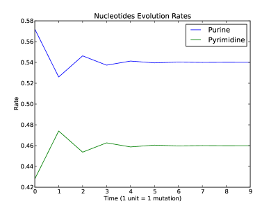
Figure 2: Prediction of purine/pyrimidine evolution of ura3 gene in non-symmetric Model of size $2\times 2$.

Theorem 1 allow us to compute the limit of the rates of purines and pyrimidines:

Computation of probability $a$.

$a=P(R\rightarrow R)=(1-m)+P(A\rightarrow G)+P(G\rightarrow A)$. The use of Table 1 implies that $a=(1-m)+m\left(\dfrac{0+26}{x}\right)$, where $x$ is such that $1-a=P(R\rightarrow Y)=m\left(\dfrac{6+8+28+9}{x}\right)$, i.e., $x=77$, and so $a=1-\dfrac{51m}{77}$.

Computation of probability $c$.

Similarly, $c=P(Y\rightarrow R)=P(C\rightarrow A)+P(C\rightarrow G)+P(T\rightarrow A)+P(T\rightarrow G)=\dfrac{70m}{y}$, whereas $1-c=1-m+\dfrac{20m}{y}$. So $c=\dfrac{7m}{9}$.

The purine/pyrimidine mutation matrix that corresponds to the data of [5] is thus equal to:

$$M=\left(\begin{array}[]{cc}1-\dfrac{51m}{77}&\dfrac{51m}{77}\\ \dfrac{7m}{9}&1-\dfrac{7m}{9}\end{array}\right).$$

Using the value of $m$ for the $ura3$ gene leads to $1-a=2.02357\times 10^{-7}$ and $c=2.37627\times 10^{-7}$, which can be used in Theorem 1 to conclude that the rate of pyrimidines is convergent to $45.992\%$ whereas the rate of purines converge to $54.008\%$. Numerical simulations using data published in [5] are given in Figure 2, leading to a similar conclusion.

3 A First Non-Symmetric Genomes Evolution Model of size $3\times 3$ having 6 Parameters

In order to investigate the evolution of the frequencies of cytosines and thymines in the gene $ura3$, a model of size $3\times 3$ compatible with real mutation rates of the yeast Saccharomyces cerevisiae is now presented.

3.1 Formalization

Let us consider a line of yeasts where a given gene is sequenced at each generation, in order to clarify explanations. The $n-$th generation is obtained at time $n$, and the rates of purines, cytosines, and tymines at time $n$ are respectively denoted by $P_{R}(n),P_{C}(n)$, and $P_{T}(n)$.

Let $a$ be the probability that a purine is changed into a cytosine between two generations, that is: $a=P(R\rightarrow C)$. Similarly, denote by $b,c,d,e,f$ the respective probabilities: $P(R\rightarrow T)$, $P(C\rightarrow R)$, $P(C\rightarrow T)$, $P(T\rightarrow R)$, and $P(T\rightarrow C)$. Contrary to existing approaches, $P(R\rightarrow C)$ is not supposed to be equal to $P(C\rightarrow R)$, and the same statement holds for the other probabilities. For the sake of simplicity, we will consider in this first research work that $a,b,c,d,e,f$ are not time dependent.

Let

$$M=\left(\begin{array}[]{ccc}1-a-b&a&b\\ c&1-c-d&d\\ e&f&1-e-f\end{array}\right)$$

be the mutation matrix associated to the probabilities mentioned above, and $P_{n}$ the vector of occurrence, at time $n$, of each of the three kind of nucleotides. In other words, $P_{n}=(P_{R}(n)~{}~{}P_{C}(n)~{}~{}P_{T}(n))$. Under that hypothesis, $P_{n}$ is a probability vector: $\forall n\in\mathbb{N},$

• $P_{R}(n),P_{C}(n),P_{T}(n)\in[0,1]$,

• $P_{R}(n)+P_{C}(n)+P_{T}(n)=1$,

Let $P_{0}=(P_{R}(0)~{}~{}P_{C}(0)~{}~{}P_{T}(0))\in[0,1]^{3}$ be the initial probability vector. We have obviously:

$$P_{R}(n+1)=P_{R}(n)P(R\rightarrow R)+P_{C}(n)P(C\rightarrow R)+P_{T}(n)P(T\rightarrow R).$$

Similarly, $P_{C}(n+1)=P_{R}(n)P(R\rightarrow C)+P_{C}(n)P(C\rightarrow C)+P_{T}(n)P(T\rightarrow C)$ and $P_{T}(n+1)=P_{R}(n)P(R\rightarrow T)+P_{C}(n)P(C\rightarrow T)+P_{T}(n)P(T\rightarrow T)$. This equality yields the following one,

$$P_{n}=P_{n-1}M=P_{0}M^{n}.$$ (4)

In all that follows we wonder if, given the parameters $a,b,c,d,e,f$ as in [5], one can determine the frequency of occurrence of any of the three kind of nucleotides when $n$ is sufficiently large, in other words if the limit of $P_{n}$ is accessible by computations.

3.2 Resolution

The characteristic polynomial of $M$ is equal to

$$\begin{array}[]{cl}\chi_{M}(x)&=x^{3}+(s-3)x^{2}+(p-2s+3)x-1+s-p\\ &=(x-1)\left(x^{2}+(s-2)x+(1-s+p)\right),\end{array}$$

where

$$s=a+b+c+d+e+f,$$

$$p=ad+ae+af+bc+bd+bf+ce+cf+de,$$

$$det(M)=1-s+p.$$

The discriminant of the polynomial of degree 2 in the factorization of $\chi_{M}$ is equal to $\Delta=(s-2)^{2}-4(1-s-p)=s^{2}-4p$. Let $x_{1}$ and $x_{2}$ the two roots (potentially complex or equal) of $\chi_{M}$, given by

$$x_{1}=\dfrac{-s+2-\sqrt{s^{2}-4p}}{2}\textrm{ and }x_{2}=\dfrac{-s+2+\sqrt{s^{2}-4p}}{2}.$$ (5)

Let $n\in\mathbb{N},n\geqslant 2$. As $\chi_{M}$ is a polynomial of degree 3, a division algorithm of $X^{n}$ by $\chi_{M}(X)$ leads to the existence and uniqueness of two polynomials $Q_{n}$ and $R_{n}$, such that

$$X^{n}=Q_{n}(X)\chi_{2}(X)+R_{n}(X),$$ (6)

where the degree of $R_{n}$ is lower than or equal to the degree of $\chi_{M}$, i.e., $R_{n}(X)=a_{n}X^{2}+b_{n}X+c_{n}$ with $a_{n},b_{n},c_{n}\in\mathbb{R}$ for every $n\in\mathbb{N}$. By evaluating (6) in the three roots of $\chi_{M}$, we find the system

$$\left\{\begin{array}[]{cl}1&=a_{n}+b_{n}+c_{n}\\ x_{1}^{n}&=a_{n}x_{1}^{2}+b_{n}x_{1}+c_{n}\\ x_{2}^{n}&=a_{n}x_{2}^{2}+b_{n}x_{2}+c_{n}\\ \end{array}\right.$$

This system is equivalent to

$$\left\{\begin{array}[]{cccccl}c_{n}&+&b_{n}&+&a_{n}&=1\\ &&b_{n}(x_{1}-1)&+&a_{n}(x_{1}^{2}-1)&=x_{1}^{n}-1\\ &&b_{n}(x_{2}-1)&+&a_{n}(x_{2}^{2}-1)&=x_{2}^{n}-1\\ \end{array}\right.$$

For the $ura3$ gene, it is easy to check that $x_{1}\neq 1$, $x_{2}\neq 1$, and $x_{1}\neq x_{2}$ (see numerical applications of Section 3.4). Then standard algebraic computations give

$$\left\{\begin{array}[]{l}a_{n}=\dfrac{1}{x_{2}-x_{1}}\left[\dfrac{x_{2}^{n}-1}{x_{2}-1}-\dfrac{x_{1}^{n}-1}{x_{1}-1}\right],\\ \\ b_{n}=\dfrac{x_{1}+1}{x_{1}-x_{2}}\dfrac{x_{2}^{n}-1}{x_{2}-1}+\dfrac{x_{2}+1}{x_{2}-x_{1}}\dfrac{x_{1}^{n}-1}{x_{1}-1},\\ \\ c_{n}=1-a_{n}-b_{n}.\end{array}\right.$$

Using for $i=1,2$ and $n\in\mathbb{N}$ the following notation,

$$X_{i}(n)=\dfrac{x_{i}^{n}-1}{x_{i}-1},$$ (7)

and since $x_{2}-x_{1}=\sqrt{\Delta}$, the system above can be rewritten as

$$\left\{\begin{array}[]{l}a_{n}=\dfrac{X_{2}(n)-X_{1}(n)}{\sqrt{\Delta}},\\ \\ b_{n}=\dfrac{(x_{2}+1)X_{1}(n)-(x_{1}+1)X_{2}(n)}{\sqrt{\Delta}},\\ \\ c_{n}=1+\dfrac{x_{1}X_{2}(n)-x_{2}X_{1}(n)}{\sqrt{\Delta}}.\end{array}\right.$$ (8)

By evaluating (6) in $M$ and due to the theorem of Cayley-Hamilton, we finally have for every integer $n\geqslant 1$,

$$M^{n}=a_{n}M^{2}+b_{n}M+c_{n}I_{3},$$ (9)

where $I_{3}$ is the identity matrix of size 3, $a_{n},b_{n},$ and $c_{n}$ are given by (8), and $M^{2}$ is given by

$$M^{2}=\left(\begin{array}[]{c|c|c}a^{2}+2ab+ac-2a&-a^{2}-ab-ac&-ab+ad-b^{2}\\ +b^{2}+be-2b+1&-ad+2a+bf&-be-bf+2b\\ \hline\cr-ac-bc-c^{2}&ac+c^{2}+2cd-2c&bc-cd-d^{2}\\ -cd+2c+de&+d^{2}+df-2d+1&-de-df+2d\\ \hline\cr-ae-be+cf&ae-cf-df&be+df+e^{2}+2ef\\ -e^{2}-ef+2e&-ef-f^{2}+2f&-2e+f^{2}-2f+1\end{array}\right).$$

3.3 Convergence study

In the case of $ura3$, $|x_{1}|<1$ and $|x_{2}|<1$ (see the next section). Then $X_{i}(n)\longrightarrow\dfrac{1}{1-x_{i}}$ for $i=1,2$ and so

$$a_{n}\longrightarrow\dfrac{1}{\sqrt{\Delta}}\left(\dfrac{1}{1-x_{2}}-\dfrac{1}{1-x_{1}}\right).$$

Denote by $a_{\infty}$ this limit. We have

$$a_{\infty}=\dfrac{x_{2}-x_{1}}{\sqrt{\Delta}(1-x_{2})(1-x_{1})}=\dfrac{1}{(1-x_{2})(1-x_{1})}=\dfrac{1}{\dfrac{s+\sqrt{\Delta}}{2}\dfrac{s-\sqrt{\Delta}}{2}},$$

and finally

$$a_{\infty}=\dfrac{4}{s^{2}-\Delta}=\dfrac{1}{p}.$$

Similarly, $b_{n}=X_{1}(n)-a_{n}(x_{1}+1)$ satisfies

$$b_{n}\longrightarrow\dfrac{1}{1-x_{1}}-\dfrac{x_{1}+1}{p}.$$

The following computations

$$\dfrac{1}{1-x_{1}}=\dfrac{2}{s+\sqrt{\Delta}}=\dfrac{2(s-\sqrt{\Delta})}{s^{2}-\Delta}=\dfrac{s-\sqrt{\Delta}}{2p},$$

$$\dfrac{x_{1}+1}{p}=\dfrac{-s+4-\sqrt{\Delta}}{2p},$$

finally yield

$$b_{\infty}=\dfrac{s-2}{p}.$$

So

$$c_{n}\longrightarrow 1-a_{\infty}-b_{\infty}=\dfrac{p-s+1}{p},$$

and to sum up, the distribution limit is given by

$$\left\{\begin{array}[]{l}a_{\infty}=\dfrac{1}{p}\\ \\ b_{\infty}=\dfrac{s-2}{p}\\ \\ c_{\infty}=\dfrac{p-s+1}{p}\end{array}\right.$$ (10)

Using the latter values in (9), we can determine the limit of $M^{n}$, which is $a_{\infty}M^{2}+b_{\infty}M+c_{\infty}I_{3}$. All computations done, we find the following limit for $M^{n}$,

$$\dfrac{1}{p-bf+df}\left(\begin{array}[]{ccc}ce+cf+de-bf+df&ae+af+bf&ad+bc+bd\\ ce+cf+de&ae+af+df&ad+bc+bd\\ ce+cf+de&ae+af+bf&ad+bc+bd-bf+df\\ \end{array}\right).$$

Using (4), we can thus finally determine the limit of $P_{n}=P_{0}M^{n}$ $=(P_{R}(0)~{}~{}P_{C}(0)~{}~{}P_{T}(0))M^{n}$, which leads to the following result.

Theorem 2

The frequencies $P_{R}(n),P_{C}(n)$, and $P_{T}(n)$ of occurrence at time $n$ of purines, cytosines, and thymines in the considered gene $ura3$ of the yeast Saccharomyces cerevisiae converge to the following values:

• $P_{R}(n)\longrightarrow\dfrac{ce+cf+de+(df-bf)P_{R}(0)}{p-bf+df}$

• $P_{C}(n)\longrightarrow\dfrac{ae+af+df+(df-bf)P_{C}(0)}{p-bf+df}$

• $P_{T}(n)\longrightarrow\dfrac{ad+bc+bd+(df-bf)P_{T}(0)}{p-bf+df}$

_□

3.4 Numerical Application and Simulations

We consider another time the numerical values for mutations published in [5]. Gene ura3 of the Yeast Saccharomyces cerevisiae has a mutation rate of $3.80\times 10^{-10}$/bp/generation [5]. As this gene is constituted by 804 nucleotides, we can deduce that its global mutation rate per generation is equal to $m=3.80\times 10^{-10}\times 804=3.0552\times 10^{-7}$. Let us compute the values of $a,b,c,d,e,$ and $f$. The first line of the mutation matrix is constituted by $1-a-b=P(R\rightarrow R)$, $a=P(R\rightarrow T)$, and $b=P(R\rightarrow C)$. $P(R\rightarrow R)$ takes into account the fact that a purine can either be preserved (no mutation, probability $1-m$), or mutate into another purine ($A\rightarrow G$, $G\rightarrow A$). As the generations pass, authors of [5] have counted 0 mutations of kind $A\rightarrow G$, and 26 mutations of kind $G\rightarrow A$. Similarly, there were 28 mutations $G\rightarrow T$ and 8: $A\rightarrow T$, so 36: $R\rightarrow T$. Finally, 6: $A\rightarrow C$ and 9: $G\rightarrow C$ lead to 15: $R\rightarrow C$ mutations. The total of mutations to consider when evaluating the first line is so equal to 77. All these considerations lead to the fact that $1-a-b=(1-m)+m\dfrac{26}{77}$, $a=\dfrac{36m}{77}$, and $b=\dfrac{15m}{77}$. A similar reasoning leads to $c=\dfrac{19m}{23}$, $d=\dfrac{4m}{23}$, $e=\dfrac{51m}{67}$, and $f=\dfrac{16m}{67}$.

In that situation, $s=a+b+c+d+e+f=\dfrac{205m}{77}\approx 8.134\times 10^{-7}$, and $p=\dfrac{207488m^{2}}{118657}\approx 1.632\times 10^{-13}.$ So $\Delta=s^{2}-4p=\dfrac{854221m^{2}}{9136589}>0$, $x_{1}=1-\dfrac{m}{2}\left(\dfrac{205}{77}+\sqrt{\dfrac{854221}{9136589}}\right)$, and $x_{2}=1-\dfrac{m}{2}\left(\dfrac{205}{77}-\sqrt{\dfrac{854221}{9136589}}\right)$. As $x_{1}\approx 0.9999685\in[0,1]$ and $x_{2}\approx 0.9999686\in[0,1]$, we have, due to Theorem 2:

• $P_{R}(n)\longrightarrow\dfrac{ce+cf+de+(df-bf)P_{R}(0)}{p-bf+df}$

• $P_{C}(n)\longrightarrow\dfrac{ae+af+df+(df-bf)P_{C}(0)}{p-bf+df}$

• $P_{T}(n)\longrightarrow\dfrac{ad+bc+bd+(df-bf)P_{T}(0)}{p-bf+df}$

Using the data of [5], we find that $P_{R}(0)=\dfrac{460}{804}\approx 0.572$, $P_{C}(0)=\dfrac{133}{804}\approx 0.165$, and $P_{T}(0)=\dfrac{211}{804}\approx 0.263$. So $P_{R}(n)\longrightarrow 0.549$, $P_{C}(n)\longrightarrow 0.292$, and $P_{T}(n)\longrightarrow 0.159$. Simulations corresponding to this example are given in Fig. 3.

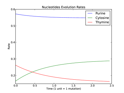
Figure 3: Prediction of evolution concerning the purine, thymine, and cytosine rates in ura3. Non-symmetric Model of size $3\times 3$.

4 Conclusion

In this document, the possible evolution of gene $ura3$ of the yeast Saccharomyces cerevisiae has been studied. As current models of nucleotides cannot fit the mutations obtained experimentally by Lang and Murray [5], authors of this paper have introduced two new simple models to predict the evolution of this gene. On the one hand, a formulation of a non symmetric discrete model of size $2\times 2$ has been proposed, which studies a DNA evolution taking into account purines and pyrimidines mutation rates. A simulation has been performed, to compare the proposal to the well known Jukes and Cantor model. On the other hand, a 6-parameters non symmetric model of size $3\times 3$ has been introduced and tested with numerical simulations, to make a distinction between cytosines and thymines in the former proposal. These two models still remain generic, and can be adapted to a large panel of applications, replacing either the couple (purines, pyrimidines) or the tuple (purines, cytosines, thymines) by any categories of interest.

The $ura3$ gene is not the unique example of a DNA sequence of interest such that none of the existing nucleotides evolution models cannot be applied due to a complex mutation matrix. For instance, a second gene called $can1$ has been studied too by the authors of [5]. Similarly to gene $ura3$, usual models cannot be used to predict the evolution of $can1$, whereas a study following a same canvas than what has been proposed in this research work can be realized. In future work, the authors’ intention is to make a complete mathematical study of the 6-parameters non symmetric model of size $3\times 3$ proposed in this document, and to apply it to various case studies. Biological consequences of the results produces by this model will be systematically investigated. Then, the most general non symmetric model of size $4$ will be regarded in some particular cases taken from biological case studies, and the possibility of mutations non uniformly distributed will then be investigated.

References

- [1] J. Felsenstein. A view of population genetics. Science, 208(4449):1253, Jun 1980.
- [2] M. Hasegawa, H. Kishino, and T. Yano. Dating of the human-ape splitting by a molecular clock of mitochondrial dna. J Mol Evol, 22(2):160–174, 1985.
- [3] T. H. Jukes and C. R. Cantor. Evolution of Protein Molecules. Academy Press, 1969.
- [4] Motoo Kimura. A simple method for estimating evolutionary rates of base substitutions through comparative studies of nucleotide sequences. Journal of Molecular Evolution, 16:111–120, 1980. 10.1007/BF01731581.
- [5] Gregory I. Lang and Andrew W. Murray. Estimating the per-base-pair mutation rate in the yeast saccharomyces cerevisiae. Genetics, 178(1):67–82, January 2008.
- [6] K Tamura. Estimation of the number of nucleotide substitutions when there are strong transition-transversion and g+c-content biases. Molecular Biology and Evolution, 9(4):678–687, 1992.
- [7] Z. Yang. Estimating the pattern of nucleotide substitution. Journal of Molecular Evolution, 10:105–111, 1994.