Bézier developable surfaces

Abstract

In this paper we address the issue of designing developable surfaces with Bézier patches. We show that developable surfaces with a polynomial edge of regression are the set of developable surfaces which can be constructed with Aumann’s algorithm. We also obtain the set of polynomial developable surfaces which can be constructed using general polynomial curves. The conclusions can be extended to spline surfaces as well.

1 Introduction

Developable surfaces are intrinsically plane surfaces, that is, they are isometric to regions of the plane [1]. Hence, lenghts, angles and areas of the plane are preserved on transforming them into developable surfaces. For this reason, they are much appreciated in the industry. Naval industry, for instance, uses plane sheets of steel and it is less expensive to fold them than to modify their curvature by other procedures involving application of heat. Textile industry uses plane sheets of cloth. And in architecture there are constructions based on developable surfaces [2]. In fact, small deviations from developability can be accepted depending on the material [3], allowing the normal to a ruled surface to vary slightly along each ruling.

However, it is not easy to deal with developable surfaces within the framework of CAGD, since the developability condition for a NURBS surface is non-linear in the vertices of its control net.

There have been several attempts to cope with this problem from different points of view.

One approach consists in restricting to classes of surfaces and their boundary curves. For instance, in [4] the developability condition is solved for low degrees of rational curves. In [5] the boundary curves are taken to be parallel and of degree three and four. Interpolating developable surfaces are constructed for them which are free of singularities. This procedure is extended to other degrees in [6]. In [7] Bézier such developable surfaces are linked with class of differentiability $C^{2}$.

Projective geometry provides an elegant approach to this problem [8]. The dual space is the set of planes in space and one can view a developable surface as the one-parameter family of the tangent planes to its rulings. The developability condition is simple in this framework [9]. This has motivated algorithms for constructing developable surfaces based on their tangent planes [10].

Another approach is the contruction of approximately developable surfaces which may be useful for the industry [11]. One way to accomplish this is the use of spline cones [12]. In [3] nearly developable spline surfaces are used for naval architecture.

Another approach is based on the de Casteljau algorithm. In [13] conditions are provided for control points of a Bézier surface to be developable, restricting its application to degrees two and three and to cylindrical and conical surfaces of arbitrary degree. Also grounded on the de Casteljau algorithm, [14] constructs generic Bézier developable surfaces through a given curve. In order to solve interpolation problems, degree-elevation is applied to the previous family of developable surfaces in [15]. The extension to spline developable surfaces, based on the De Boor algorithm, is provided in [16, 17].

In this paper we would like to show to what extent Aumann’s family of Bézier developable surfaces is general. We show that developable surfaces with a polynomial edge of regression are the ones which can be constructed with Aumann’s algorithm. Furthermore, we would like to know if there are other constructions of Bézier developable surfaces, based on general Bézier curves, which allow free parameters for design. We find a family of surfaces in addition to the ones available with Aumann’s algorithm.

The paper is organised in the following way: In Section 2 we review the main properties of developable surfaces in differential geometry. In Section 3 we interpret the developability condition for Bézier surfaces, producing an straightforward method for exporting results from differential geometry to CAGD. An algebraic parametric equation for the edge of regression of a Bézier developable surface is obtained. In Section 4 we review transformations which can be performed on patches of developable surfaces. Several families of Bézier developable surfaces are studied in Section 5. In particular, we characterise Aumann’s family in terms of their edge of regression. Finally, we study polynomial developable surfaces using differential equations in order to produce families of surfaces with free parameters based on general polynomial curves.

The results in this paper are obtained for polynomial developable surfaces. Since spline developable surfaces are characterised in a similar fashion [16], the results are valid for the spline case too.

2 Developable surfaces

A ruled surface bounded by two curves parametrised by $c(u)$, $d(u)$ is the surface formed by the segments, named rulings, linking points with the same parameter $u$ on both curves. They can be parametrised as

$$b(u,v)=(1-v)c(u)+vd(u),\quad u,v\in[0,1].$$ (1)

Reparametrisation of the curves allows for different ruled surfaces. Hence our starting point are the parametrised curves, fixing the parametrisation from the beginning. A non-polynomial reparametrisation would cast the parametrised surface out of the Bézier formalism.

The tangent plane to the ruled surface usually varies from one point to another along a ruling. Developable surfaces [1] are ruled surfaces for which the tangent plane is constant along each ruling. This is accomplished if the vectors $c^{\prime}(u)$, $d^{\prime}(u)$ and $\mathbf{v}(u):=d(u)-c(u)$ are coplanary for all values of $u$.

This is easily seen, since at $v=0$ the tangent plane is spanned by $\mathbf{v}(u)$ and $c^{\prime}(u)$ and at $v=1$ it is spanned by $\mathbf{v}(u)$ and $d^{\prime}(u)$. If these tangent planes are the same, it is the same for all points on a ruling.

Hence, for developable surfaces, the vectors $c^{\prime}(u)$, $\mathbf{v}(u)$ and $\mathbf{v}^{\prime}(u)$ are linearly dependent. For non-cylindrical surfaces we get

$$c^{\prime}(u)=\lambda(u)\mathbf{v}(u)+\mu(u)\mathbf{v}^{\prime}(u).$$ (2)

Accordingly, there are several types of developable surfaces:

1. Planar surfaces: Plane regions.

2. Cylinders: Developable surfaces with parallel rulings.

3. Cones: Developable surfaces for which all rulings intersect at a point named vertex.

4. Tangent surfaces: Developable surfaces spanned by the tangent lines to a curve, named edge of regression.

Equation (2) can be simplified by choosing a different curve on the developable surface, $r(u)=c(u)-\mu(u)\mathbf{v}(u)$,

$$r^{\prime}(u)=\left(\lambda(u)-\mu^{\prime}(u)\right)\mathbf{v}(u).$$ (3)

Except for the case $\lambda(u)\equiv\mu^{\prime}(u)$ or $r^{\prime}(u)\equiv 0$, i.e., except for the case that $r(u)$ describes the vertex of a cone, Equation (3) describes the tangent surface to $r(u)$, which is the edge of regression of the developable surface. We see that tangent surfaces are the general case of developable surfaces. In most of this paper it will be the only case that we consider.

3 Bézier developable patches

The parametrisation $c(u)$ of a Bézier curve of degree $n$ and control polygon $\{c_{0},\ldots,c_{n}\}$ can be contructed using the de Casteljau algorithm [18] in $n$ iterations,

$$c^{1)}_{i}(u) = (1-u)c_{i}+uc_{i+1},\ i=0,\ldots,n-1,$$

$$c^{r)}_{i}(u) = (1-u)c^{r-1)}_{i}(u)+uc^{r-1)}_{i+1}(u)\ i=0,\ldots,n-r,$$

$$c(u) := c^{n)}_{0}(u)=(1-u)c^{n-1)}_{0}(u)+uc^{n-1)}_{1}(u).$$ (4)

The algorithm also provides the derivative of the curve as the difference of the two points in the last-but-one iteration,

$$c^{\prime}(u)=n\left(c_{1}^{n-1)}(u)-c_{0}^{n-1)}(u)\right).$$ (5)

If we consider now two Bézier curves $c(u)$ and $d(u)$ of degree $n$ as boundary curves of a ruled surface patch, the developability condition of coplanarity of vectors $c^{\prime}(u)$, $d^{\prime}(u)$, $d(u)-c(u)$ is equivalent to the condition of coplanarity of points $c^{n-1)}_{0}(u)$, $c^{n-1)}_{1}(u)$, $d^{n-1)}_{0}(u)$, $d^{n-1)}_{1}(u)$. See Fig 1.

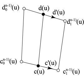
Figure 1: Coplanarity condition and developability

This coplanarity condition can be written in terms of two functions $\Lambda(u)$, $M(u)$, such that

$$\left(1-\Lambda(u)\right)c_{0}^{n-1)}(u)+\Lambda(u)c_{1}^{n-1)}(u)=\left(1-M(u)\right)d_{0}^{n-1)}(u)+M(u)d_{1}^{n-1)}(u),$$

except for some cases of cones.

The use of blossoms

$$c^{1)}_{i}[u_{1}] := c^{1)}_{i}(u_{1})=(1-u_{1})c_{i}+u_{1}c_{i+1},\quad i=0,\ldots,n-1,$$

$$c^{r)}_{i}[u_{1},\ldots,u_{r}] := (1-u_{r})c_{i}^{r-1)}[u_{1},\ldots,u_{r-1}]+u_{r}c_{i+1}^{r-1)}[u_{1},\ldots,u_{r-1}],$$

$$c[u_{1},\ldots,u_{n}] := c^{n)}_{0}[u_{1},\ldots,u_{n}]\ ,\quad i=0,\ldots,n-r,\quad r=1,\ldots,n,$$ (6)

to write the last-but-one vertices of the de Casteljau algorithm,

$$c_{0}^{n-1)}(u)=c[u^{<n-1>},0]\ ,\qquad c_{1}^{n-1)}(u)=c[u^{<n-1>},1]\ ,$$

allow a simpler expression for the coplanarity condition [19]:

Theorem 1

Two Bézier curves $c(u)$, $d(u)$ of degree $n$ and vertices $\{c_{0},\ldots,c_{n}\}$, $\{d_{0},\ldots,d_{n}\}$ are the boundary curves of a generic developable surface patch if and only if their respective blossoms are related by

$$c[u^{<n-1>},\Lambda(u)]=d[u^{<n-1>},M(u)].$$

This construction of developable surfaces has nice features, which are based on the use of blossoms. Algorithms grounded on blossoms are compatible with this construction.

These functions $\Lambda(u)$, $M(u)$ are closely related to the ones in (2). If we write that equation in terms of blossoms for curves of degree $n$,

$$0 = c^{\prime}(u)-\lambda(u)\mathbf{v}(u)-\mu(u)\mathbf{v}^{\prime}(u)$$

$$= n\left(c[u^{<n-1>},1]-c[u^{<n-1>},0]\right)$$

$$- \lambda(u)\left(d[u^{<n>}]-c[u^{<n>}]\right)$$

$$- n\mu(u)\left(d[u^{<n-1>},1]-d[u^{<n-1>},0]\right.$$

$$- \left.c[u^{<n-1>},1]+c[u^{<n-1>},0]\right),$$

and using the de Casteljau algorithm (3) for expanding the expressions for $c(u)$ and $d(u)$, we may collect the terms,

$$c[u^{<n-1>},1]\left(n+u\lambda(u)+n\mu(u)\right)$$

$$+ c[u^{<n-1>},0]\left((1-u)\lambda(u)-n-n\mu(u)\right)$$

$$= d[u^{<n-1>},1]\left(n\mu(u)+u\lambda(u)\right)$$

$$+ d[u^{<n-1>},0]\left((1-u)\lambda(u)-n\mu(u)\right),$$

so that we may simplify the blossoms using affine combinations,

$$c\left[u^{<n-1>},\frac{n+n\mu(u)+u\lambda(u)}{\lambda(u)}\right]=d\left[u^{<n-1>},\frac{n\mu(u)+u\lambda(u)}{\lambda(u)}\right].$$

If we compare this expression with Theorem 1, we get:

Proposition 1

A developable surface parametrised as $b(u,v)=c(u)+v\mathbf{v}(u)$, with $\mathbf{v}(u)=d(u)-c(u)$, where $c(u)$, $d(u)$ are curves of degree $n$, satisfying Theorem 1 for some rational functions $\Lambda(u)$, $M(u)$ has functions $\lambda(u)$, $\mu(u)$ in (2) related by

$$\Lambda(u)=\frac{n(\mu(u)+1)+u\lambda(u)}{\lambda(u)},\ M(u)=\frac{n\mu(u)+u\lambda(u)}{\lambda(u)},$$ (7)

$$\lambda(u)=\frac{n}{\Lambda(u)-M(u)},\quad\mu(u)=\frac{M(u)-u}{\Lambda(u)-M(u)}.$$ (8)

In this sense we may view Theorem 1 as a way of writing the differential equation (2) for polynomial curves in an algebraic fashion. This provides an interpretation for $\Lambda(u)$, $M(u)$ and it is useful to exchange results between the general and the polynomial case.

We may also characterise the edge of regression of a Bézier developable surface in terms of the functions $\Lambda(u)$, $M(u)$.

The edge of regression of a developable surface is formed by the set of points where the surface is singular, two-sheeted more precisely, as we see in Fig. 2. It is therefore of great importance for design to keep it under control in order to produce smooth surfaces.

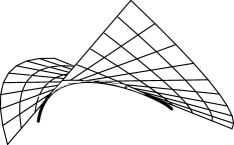
Figure 2: Edge of regression and two sheets of a developable surface

We may locate it by searching the points where the parametrisation $b(u,v)$ of the developable surface is degenerate because its partial derivatives are parallel,

$$b_{u}(u,v)=(1-v)c^{\prime}(u)+vd^{\prime}(u)\ ,\quad b_{v}(u,v)=d(u)-c(u)\ .$$

Since

$$b_{u}(u,v) = n(1-v)\left(c^{n-1)}_{1}(u)-c^{n-1)}_{0}(u)\right)$$

$$+ nv\left(d^{n-1)}_{1}(u)-d^{n-1)}_{0}(u)\right),$$

$$b_{v}(u,v) = (1-u)\left\{d^{n-1)}_{0}(u)-c^{n-1)}_{0}(u)\right\}$$

$$+ u\left\{d^{n-1)}_{1}(u)-c^{n-1)}_{1}(u)\right\},$$

parallelism between these two vectors implies the existence of a factor $\alpha(u,v)$ such that $\alpha nb_{v}=b_{u}$,

$$\left(1-u+\frac{v-1}{\alpha}\right)c^{n-1)}_{0}(u)+\left(\frac{1-v}{\alpha}+u\right)c^{n-1)}_{1}(u)$$

$$= \left(1-u+\frac{v}{\alpha}\right)d^{n-1)}_{0}(u)+\left(u-\frac{v}{\alpha}\right)d^{n-1)}_{1}(u)$$

On the other hand the developability condition imposes another barycentric combination,

$$(1-\Lambda(u))c^{n-1)}_{0}(u)+\Lambda(u)c^{n-1)}_{1}(u)=(1-M(u))d^{n-1)}_{0}(u)+M(u)d^{n-1)}_{1}(u),$$

which allows us to read the unknown $\alpha$

$$\Lambda(u)=\frac{1-v}{\alpha(u,v)}+u,\quad M(u)=u-\frac{v}{\alpha(u,v)},$$

and write down the parametric equations for the edge of regression:

Proposition 2

A developable surface parametrised by $b(u,v)=(1-v)c(u)+vd(u)$ where $c(u)$, $d(u)$ are polynomial curves of degree $n$ with blossoms related by $c[u^{<n-1>},\Lambda(u)]=d[u^{<n-1>},M(u)]$ for some functions $\Lambda$, $M$ has as edge of regression the line given by the parametric equation

$$v=\frac{u-M(u)}{\Lambda(u)-M(u)}.$$ (9)

This is interesting, since it allows control of the position of the edge of regression in order to keep our patch away from it, preventing the rulings from intersecting it and ruining the surface patch.

In the constant case [14] it implies that the edge of regression is a line of degree $n+1$ on the developable surface, unless $\Lambda$ equals $M$.

The equation for the edge of regression is algebraic and simple enough to simplify the task of avoiding this singular line when designing with developable surfaces.

4 Operations with Bézier developable surfaces

The functions $\Lambda(u)$ and $M(u)$ depend on the patch for the developable surface. A developable surface has different functions $\Lambda(u)$ and $M(u)$ when considering patches with different boundary curves.

There are a number of simple operations that we may perform on developable surfaces in order to modify the coordinate patch:

• Restriction of parameter $v$ to $[a,b]\subset[0,1]$: If we restrict the parametrisation of the developable surface through $v\in[a,b]$ (Fig. 3), the new boundary curves are

  $$\tilde{c}(u)=(1-a)c(u)+ad(u),\quad\tilde{d}(u)=(1-b)c(u)+bd(u),$$

  and their blossoms are related by Theorem 1 with new functions $\tilde{\Lambda}(u)$, $\tilde{M}(u)$,

  $$\tilde{c}[u^{<n-1>},\tilde{\Lambda}(u)]=\tilde{d}[u^{<n-1>},\tilde{M}(u)],$$

  which in terms of the blossoms of $c(u)$ and $d(u)$,

  $$c\left[u^{<n-1>},\frac{(1-a)\tilde{\Lambda}(u)+(b-1)\tilde{M}(u)}{b-a}\right]=d\left[u^{<n-1>},\frac{b\tilde{M}(u)-a\tilde{\Lambda}(u)}{b-a}\right],$$

  allows reading the functions $\Lambda(u)$, $M(u)$ after comparing with the developability condition in Theorem 1,

  $$\Lambda(u)=\frac{(1-a)\tilde{\Lambda}(u)+(b-1)\tilde{M}(u)}{b-a},\quad M(u)=\frac{b\tilde{M}(u)-a\tilde{\Lambda}(u)}{b-a},$$

  which provide the new functions $\tilde{\Lambda}(u)$, $\tilde{M}(u)$,

  $$\tilde{\Lambda}(u)=b\Lambda(u)+(1-b)M(u),\qquad\tilde{M}(u)=a\Lambda(u)+(1-a)M(u).$$ (10)

  

  Figure 3: Restriction of parameter $v$ on a developable surface

• Restriction of parameter $u$ to $[a,b]\subset[0,1]$: This is equivalent to an affine change of parameter $u=(1-\tilde{u})a+\tilde{u}b$, $\tilde{u}\in[0,1]$ (Fig. 4). Since blossoms are multi-affine, this applies directly to the relation between the functions $\Lambda(u)$, $M(u)$ and the new ones,

  $$\Lambda(u)=\left(1-\tilde{\Lambda}(u)\right)a+\tilde{\Lambda}(u)b\ ,\qquad M(u)=\left(1-\tilde{M}(u)\right)a+\tilde{M}(u)b,$$

  $$\tilde{\Lambda}(u)=\frac{\Lambda(u)-a}{b-a}\ ,\quad\tilde{M}(u)=\frac{M(u)-a}{b-a}\ .$$ (11)

  

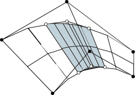
  Figure 4: Restriction of parameter $u$ on a developable surface

• Degree elevation: We know [18] that if we elevate the degree of a curve $c(u)$ from $n$ to $n+1$, the degree-elevated blossom of degree $n$ can be written in terms of the original blossom,

  $$c^{1}[u_{1},\ldots,u_{n+1}]=\frac{c[u_{1},\ldots,u_{n}]+\cdots+c[u_{2},\ldots,u_{n+1}]}{n+1}.$$

  If we consider a developable surface spanned by two curves of degree $n$ $c(u)$, $d(u)$ with functions $\Lambda(u)$, $M(u)$ and elevate the degree of both curves to $n+1$ (See Fig. 5), their blossoms have to satisfy the developability condition with new functions $\Lambda^{1}(u)$, $M^{1}(u)$,

  $$c^{1}[u^{<n>},\Lambda^{1}(u)]=d^{1}[u^{<n>},M^{1}(u)],$$

  which may be written again in terms of the original blossoms using barycentric combinations,

  $$c^{1}[u^{<n>},\Lambda^{1}(u)] = \frac{nc[u^{<n-1>},\Lambda^{1}(u)]+c[u^{<n>}]}{n+1}$$

  $$= c\left[u^{<n-1>},\frac{n\Lambda^{1}(u)+u}{n+1}\right].$$

  

  Figure 5: Degree elevation of a developable surface

  The degree-elevated developability condition just states then

  $$c\left[u^{<n-1>},\frac{n\Lambda^{1}(u)+u}{n+1}\right]=d\left[u^{<n-1>},\frac{nM^{1}(u)+u}{n+1}\right]\ ,$$

  and, compared with the former condition in Theorem 1, allows us to express the new functions $\Lambda^{1}(u)$, $M^{1}(u)$ in terms of the previous $\Lambda(u)$, $M(u)$,

  $$\Lambda^{1}(u)=\frac{(n+1)\Lambda(u)-u}{n},\qquad M^{1}(u) = \frac{(n+1)M(u)-u}{n}.$$ (12)

  This result could be derived in a different fashion. Since in equation (2) coefficients $\lambda(u)$, $\mu(u)$ are not altered by formal degree elevation,

  $$\lambda(u) = \frac{n+1}{\Lambda^{1}(u)-M^{1}(u)}=\frac{n}{\Lambda(u)-M(u)},$$

  $$\mu(u) = \frac{M^{1}(u)-u}{\Lambda^{1}(u)-M^{1}(u)}=\frac{M(u)-u}{\Lambda(u)-M(u)},$$

  we can obtain from them the expressions for $\Lambda^{1}(u)$ and $M^{1}(u)$.

  Repeated degree elevation can be also performed:

  Proposition 3

  A developable surface spanned by two curves $c(u)$, $d(u)$ of degree $n$ with functions $\Lambda(u)$ and $M(u)$ has functions

  $$\Lambda^{m}(u) = \frac{(n+m)\Lambda(u)-mu}{n},$$

  $$M^{m}(u) = \frac{(n+m)M(u)-mu}{n},$$ (13)

  after formally elevating the degree of the curves to $n+m$.

• Modification of the length of the rulings: If we rewrite the parametrisation of a ruled surface interpolating two curves $c(u)$, $d(u)$ in terms of the direction of the rulings, $\mathbf{v}(u)=d(u)-c(u)$, we may modify the surface patch (See Fig. 6) by changing the length of the vector $\mathbf{v}(u)$ through a factor $h(u)$ depending on the ruling, $\tilde{\mathbf{v}}(u)=h(u)\mathbf{v}(u)$,

  $$\tilde{b}(u,v)=c(u)+v\,h(u)\mathbf{v}(u),$$

  and the edge of the surface patch moves to the curve

  $$\tilde{d}(u)=h(u)d(u)+\left(1-h(u)\right)c(u)\ .$$

  $$\tilde{\Lambda}(u)=b\Lambda(u)+(1-b)M(u),\qquad\tilde{M}(u)=a\Lambda(u)+(1-a)M(u).$$ (14)

  

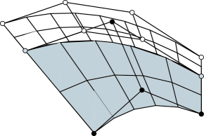
  Figure 6: Modification of the length of the rulings of a developable surface

  This procedure is useful, not only for developable surfaces, but for ruled surfaces in general.

  We compare the linear differential equation for the new patch with the original one,

  $$\lambda\mathbf{v}+\mu\mathbf{v}^{\prime}=c^{\prime}=\tilde{\lambda}\tilde{\mathbf{v}}+\tilde{\mu}\tilde{\mathbf{v}}^{\prime}=\left(\tilde{\lambda}h+\tilde{\mu}h^{\prime}\right)\mathbf{v}+\tilde{\mu}h\mathbf{v}^{\prime},$$

  in order to relate the old coefficients with the new ones,

  $$\lambda=\tilde{\lambda}h+\tilde{\mu}h^{\prime}=\frac{n}{\Lambda-M},\quad\mu=\tilde{\mu}h=\frac{M-u}{\Lambda-M},$$

  $$\tilde{\lambda}=\frac{h\lambda-h^{\prime}\mu}{h^{2}}=\frac{n+m}{\tilde{\Lambda}-\tilde{M}},\qquad\tilde{\mu}=\frac{\mu}{h}=\frac{\tilde{M}-u}{\tilde{\Lambda}-\tilde{M}},$$

  where we have assumed that $h$ is a polynomial factor of degree $m$.

  This leads to relations between the functions $\Lambda$, $M$ of both patches,

  $$\tilde{\Lambda}(u)=u+\frac{(n+m)h^{2}(u)(\Lambda(u)-M(u))+(n+m)h(u)(M(u)-u)}{nh(u)-h^{\prime}(u)(M(u)-u)},$$

  $$\tilde{M}(u)=u+\frac{(n+m)h(u)(M(u)-u)}{nh(u)-h^{\prime}(u)(M(u)-u)},$$

  Obviously, in the case of no enlargement, $h(u)\equiv 1$, the degree elevation formula (12) is recovered. This operation has been used in [15] for modifying developable patches.

• Change of parameter: If we carry out the change of parameter $u=h(U)$, where $h$ is a polynomial function of degree $m$, the degree of a polynomial developable surface through a curve $c(u)$ of degree $n$ changes from $(n,1)$ to $(mn,1)$. The new differential equation for $\hat{c}(U)=c\left(h(U)\right)$, $\hat{\mathbf{v}}(U)=\mathbf{v}\left(h(U)\right)$,

  $$\frac{d\hat{c}(U)}{dU} = h^{\prime}(U)\left.\frac{dc(u)}{du}\right|_{h(U)}=h^{\prime}(U)\left.\left(\lambda\mathbf{v}+\mu\frac{d\mathbf{v}}{du}\right)\right|_{u=h(U)}$$

  $$= h^{\prime}(U)\lambda(h(U))\hat{\mathbf{v}}(U)+\mu(h(U))\frac{d\hat{\mathbf{v}}(U)}{dU}$$

  $$= \hat{\lambda}(U)\hat{\mathbf{v}}(U)+\hat{\mu}(U)\frac{d\hat{\mathbf{v}}(U)}{dU},$$

  allows us a relation between the coefficients,

  $$\hat{\lambda}(U)=h^{\prime}(U)\lambda\left(h(U)\right),\qquad\hat{\mu}(U)=\mu\left(h(U)\right),$$

  which is translated to the functions $\Lambda$, $M$,

  $$\hat{\Lambda}(U)=\frac{m\left(\Lambda(h(U))-h(U)\right)}{h^{\prime}(U)}+U,$$

  $$\hat{M}(U)=\frac{m\left(M(h(U))-h(U)\right)}{h^{\prime}(U)}+U.$$

  For instance, in the simple case $h(U)=U^{m}$,

  $$\hat{\Lambda}(U)=\frac{\Lambda(U^{m})}{U^{m-1}},\qquad\hat{M}(U)=\frac{M(U^{m})}{U^{m-1}}.$$

5 Some Bézier developable surfaces

5.1 Bézier cylinders

The simplest example of developable surfaces are cylinders, for which all the rulings are parallel to a constant vector $\mathbf{v}$.

In the Bézier case, if $\{c_{0},\ldots,c_{n}\}$, $\{d_{0},\ldots,d_{n}\}$ are the control polygons of the boundary curves, this implies that all vectors $d_{i}-c_{i}$, $i=0,\ldots,n$ are parallel to $\mathbf{v}$ (See Fig. 7).

This implies that the differences $d^{n-1)}_{1}(u)-c^{n-1)}_{1}(u)$, $d^{n-1)}_{0}(u)-c^{n-1)}_{0}(u)$ must be parallel for all $u$,

$$d^{n-1)}_{1}(u)-c^{n-1)}_{1}(u)=\alpha(u)\left(d^{n-1)}_{0}(u)-c^{n-1)}_{0}(u)\right).$$

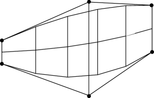
Figure 7: Bézier cylinder

In terms of blossoms,

$$c[u^{<n-1>},1]-\alpha(u)c[u^{<n-1>},0]=d[u^{<n-1>},1]-\alpha(u)d[u^{<n-1>},0],$$

the property of multi-affinity allows writing it in a compact fashion,

$$c[u^{<n-1>},\Lambda(u)]=d[u^{<n-1>},\Lambda(u)],\qquad\Lambda(u)=\frac{\alpha(u)}{\alpha(u)-1},$$

except for the simplest case $\alpha(u)\equiv 1$, that is, constant $d_{i}-c_{i}=\mathbf{v}$, $i=0,\ldots,n$.

Hence, Bézier cylinders are developable surfaces with $\Lambda\equiv M$.

Constructing a cylinder with direction $\mathbf{v}$ is easy, $d(u)=c(u)+f(u)\mathbf{v}$, where $f(u)$ can be any function. If we require the parametrisation to be polynomial of degree $n$ in $u$, $f(u)$ is a polynomial of degree equal or lower than $n$. We may relate $f(u)$ with the function $\Lambda(u)$ defining the developable surface. Comparing

$$d(u)-c(u)=f(u)\,\mathbf{v},\qquad d[u^{<n-1>},\Lambda(u)]=c[u^{<n-1>},\Lambda(u)],$$

we learn that the polar form of $f$ is to fullfil

$$f[u^{<n-1>},\Lambda(u)]\equiv 0.$$

For $f(u)=\displaystyle\sum_{i=0}^{n}a_{i}u^{i}$, the previous condition on the polarisation of $f$ reads

$$0=f[u^{<n-1>},\Lambda(u)]=a_{0}+\sum_{i=1}^{n}\frac{a_{i}}{n}\left((n-i)u^{i}+i\Lambda(u)u^{i-1}\right),$$

from which we can read the expression for $\Lambda(u)$,

$$\Lambda(u)=-\frac{\displaystyle\sum_{i=0}^{n-1}(n-i)a_{i}u^{i}}{\displaystyle\sum_{i=1}^{n}ia_{i}u^{i-1}}.$$

In particular, for $f(u)=(au+b)^{n}$, we get the constant case $\Lambda=-b/a$.

5.2 Bézier cones

As we have seen, cones are the subcase of developable surfaces with coefficients $\lambda(u)$, $\mu(u)$ related by $\lambda(u)=\mu^{\prime}(u)$. That is, $c^{\prime}(u)=\left(\mu(u)\mathbf{v}(u)\right)^{\prime}$.

The simplest cone patch is the one bounded by a curve $c(u)$ with vertex at a point $V$. The rulings have $\mathbf{v}(u)=c(u)-V$ as tangent vector, but we can construct more general patches using $\mathbf{v}(u)=(c(u)-V)f(u)$, for which

$$\lambda(u)=-\frac{f^{\prime}(u)}{f(u)},\qquad\mu(u)=\frac{1}{f(u)}.$$

If $c(u)$ is a curve of degree $n$, $c(u)-V$ is also of degree $n$ and except for constant $f$, modification of the patch implies raising its degree,

$$\Lambda(u)=\frac{f^{\prime}(u)u-(n+m)(f(u)+f^{2}(u))}{f^{\prime}(u)},\quad M(u)=\frac{f^{\prime}(u)u-(n+m)f(u)}{f^{\prime}(u)},$$

if $f(u)$ is of degree $m$.

The simple case of constant $f$, for which $d(u)$ is a scaled copy of $c(u)$ is out of this framework.

In the linear case, $f(u)=au+b$,

$$\Lambda(u)=-\frac{(n+1)^{2}(au+b)^{2}+nau+(n+1)b}{a},\qquad M(u)=-\frac{nau+(n+1)b}{a}.$$

5.3 Tangent surfaces

We start with the simple case of the tangent surface to a curve $c(u)$ of degree $n$,

$$b(u,v)=c(u)+vf(u)c^{\prime}(u),$$

which is a surface of degree $(n,1)$ provided that the factor in $\mathbf{v}(u)$ is linear: $f(u)=au+b$.

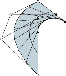
Figure 8: Tangent surface to a curve

In this case, $c^{\prime}(u)=\mathbf{v}(u)/f(u)$ and we can read directly the functions $\lambda(u)=1/f(u)$, $\mu(u)=0$, and hence

$$\Lambda(u)=u+nf(u),\qquad M(u)=u.$$

For the simplest case of $f(u)\equiv 1$ we have $\Lambda(u)=u+n$, $M(u)=u$. (See Fig. 8).

5.4 Case of constant $\Lambda$ and $M$

This is the simple case that has been explored in [14] and extended to spline surfaces in [16]. This family has the remarkable property of having linear constraints between the vertices of the cells of the control net for the surface. If $\{c_{0},\ldots,c_{n}\}$, $\{d_{0},\ldots,d_{n}\}$ are the control polygons for curves $c(u)$ and $d(u)$, Theorem 1

$$c[u^{<n-1>},\Lambda]=d[u^{<n-1>},M]$$

implies we have a set of $n$ conditions,

$$(1-\Lambda)c_{i}+\Lambda c_{i+1}=(1-M)d_{i}+Md_{i+1},\ i=0,\ldots,n-1,$$

which require that the cells of the surface are planar and that the coefficients for the combinations of the vertices are the same for all cells (See Fig. 9 for an example).

Figure 9: Developable surface with constant $\Lambda$, $M$ of degree two

The general solution to the linear differential equation (2) for these developable surfaces,

$$c^{\prime}(u)=\frac{n}{\Lambda-M}\mathbf{v}(u)+\frac{M-u}{\Lambda-M}\mathbf{v}^{\prime}(u),$$

can be split into the general solution to the homogeneous equation

$$n\mathbf{v}_{\mathrm{h}}(u)+(M-u)\mathbf{v}_{\mathrm{h}}^{\prime}(u)=0\Rightarrow\mathbf{v}_{\mathrm{h}}(u)=(M-u)^{n}\mathbf{w},$$

where $\mathbf{w}$ is an arbitrary constant vector,

$$\mathbf{v}(u)=(M-u)^{n}\mathbf{w}+\mathbf{v}_{\mathrm{p}}(u),$$

and a particular solution of the whole inhomogeneous equation, $\mathbf{v}_{\mathrm{p}}(u)$, which we may choose of degree lower than $n$. Hence, the general case is that of $\mathbf{v}$ of degree $n$, except for the specific case with $\mathbf{w}=0$.

The edge of regression for such developable surfaces,

$$r(u)=c(u)+\frac{u-M}{\Lambda-M}(d(u)-c(u)),$$

is a polynomial curve with velocity

$$r^{\prime}(u)=\frac{n+1}{\Lambda-M}(d(u)-c(u)),$$

according to (3).

If $\mathbf{v}(u)$ is of degree $n$, the edge of regression is of degree $n+1$. This poses a paradoxical question, since the developable surface of degree $n$ in $u$ is of degree $(n+1,1)$ in $u$ as tangent surface to its edge of regression.

In order to explain this issue, we show next that the tangent surface to a polynomial curve of degree $n+1$ can always be parametrised as a surface patch of degree $(n,1)$:

We start then with the tangent surface to a curve $r(u)$ of degree $n+1$ and define a surface patch on it, limited by two curves,

$$c(u)=r(u)+(au+b_{1})r^{\prime}(u),\quad d(u)=r(u)+(au+b_{2})r^{\prime}(u),$$

so that we do not change the degree of the generator of the rulings,

$$\mathbf{v}(u)=d(u)-c(u)=(b_{2}-b_{1})r^{\prime}(u).$$

It is clear that we must have $a=-1/(n+1)$ in order to lower the degree of $c(u)$ and $d(u)$.

From the differential equation governing this patch,

$$c^{\prime}(u)=\lambda(u)\mathbf{v}(u)+\mu(u)\mathbf{v}^{\prime}(u)=(1+a)r^{\prime}(u)+(au+b_{1})r^{\prime\prime}(u),$$

we may read the coefficients $\lambda$, $\mu$,

$$\lambda(u)=\frac{1+a}{b_{2}-b_{1}},\qquad\mu(u)=\frac{au+b_{1}}{b_{2}-b_{1}},$$

and hence the functions for the discrete version of it,

$$\Lambda^{1}(u)=\frac{\left(a(n+2)+1\right)u+(n+1)b_{2}}{a+1},$$

$$M^{1}(u)=\frac{\left(a(n+2)+1\right)u+(n+1)b_{1}}{a+1},$$ (15)

considering that $c(u)$ and $d(u)$ are formally of degree $n+1$.

Since we want a surface patch of degree $(n,1)$, that is, with boundary curves of degree $n$, functions $\Lambda^{1}(u)$, $M^{1}(u)$ should correspond to a degree elevation (12). This is accomplished if $a=-1/(n+1)$,

$$\Lambda^{1}(u)=\frac{(n+1)^{2}b_{2}-u}{n},\qquad M^{1}(u)=\frac{(n+1)^{2}b_{1}-u}{n},$$

which corresponds to a surface patch bounded by two curves $c(u)$, $d(u)$ of degree $n$ and constant functions

$$\Lambda=(n+1)b_{2},\qquad M=(n+1)b_{1}.$$

Hence we have proven that any tangent surface to a polynomial curve of degree $n+1$ can be put in the form of a surface patch of degree $(n,1)$ with constant values of $\Lambda$, $M$.

Since, on the other hand, developable patches with constant $\Lambda$, $M$ have polynomial edges of regression, we have:

Theorem 2

The set of developable surfaces with patches generated by two curves $c(u)$, $d(u)$ of degree $n$, with ruling generators $\mathbf{v}(u)=d(u)-c(u)$ also of degree $n$ and blossoms related by

$$c[u^{<n-1>},\Lambda]=d[u^{<n-1>},M],$$

with constant $\Lambda$, $M$ is the set of tangent surfaces to polynomial curves of degree $n+1$.

That is, Aumann’s algorithm allows construction of every developable surface with polynomial edge of regression (See Fig. 10).

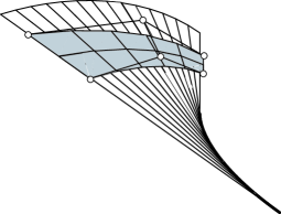
Figure 10: Constant $\Lambda$, $M$ surface as a patch of the tangent surface to a polynomial curve

Besides the previous case, there are other patches with constant functions $\Lambda$, $M$, but these are of degree $(n+1,1)$.

For instance, for $a=-1/(n+2)$ in (15), we get

$$\Lambda=(n+2)b_{2},\qquad M=(n+2)b_{1},$$

without invoking degree elevation of curves $c(u)$, $d(u)$.

This is a degenerated case for which $c(u)$, $d(u)$ are of degree $n+1$ whereas $\mathbf{v}(u)$ is of degree $n$.

Furthermore, for $a=-1/(n+m)$, we get

$$\Lambda^{2-m}(u)=\frac{(n+1)(n+m)b_{2}+(m-2)u}{n+m-1},$$

$$M^{2-m}(u)=\frac{(n+1)(n+m)b_{1}+(m-2)u}{n+m-1},$$

which correspond, after degree elevation from $n+1$ to $n+m-1$, to

$$\Lambda=(n+m)b_{2},\qquad M=(n+m)b_{1}.$$

That is, this surface patch is bounded by two curves of degree $n+1$, with blossoms related by constant values of $\Lambda$ and $M$, after formally raising their degree $m-2$ times. Since the generator of the rulings $\mathbf{v}(u)$ is of degree $n$, this is again a degenerated case.

6 General polynomial developable surfaces

According to Equation (9), Bézier developable surfaces have in principle a rational edge of regression.

We have seen that we can use for design Bézier developable surfaces with a polynomial edge of regression. First, we define the surface resorting to Aumann’s construction. Second, we modify the resulting surface patch with the operations described in Section 4. Since Theorem 1 imposes $n$ conditions on the control points of the boundary curves, this means that we can prescribe [14], for instance, just the control polygon of one of the curves, $c_{0},\ldots,c_{n}$, and one control point of the other curve, $d_{0}$. Prescribing the values of $\Lambda$ and $M$ is equivalent to prescribe $d_{1}$ in the plane defined by $c_{0},c_{1},d_{0}$.

However, Bézier developable surfaces with a rational edge of regression fall out of this construction.

It would be interesting to check if there are other constructions of polynomial developable surfaces which can be applied to Bézier curves without imposing restrictions on them and that they leave enough degrees of freedom for design.

With this aim in mind, we write the general solution of the linear differential equation (2) in a convenient form. Since it is linear, we may split it as

$$\mathbf{v}(u)=\mathbf{v}_{\mathrm{h}}(u)+\mathbf{v}_{\mathrm{p}}(u),$$ (16)

where $\mathbf{v}_{\mathrm{h}}(u)$ is the general solution of the homogeneous equation and $\mathbf{v}_{\mathrm{p}}(u)$ is one particular solution of the inhomogeneous equation.

The general solution of the homogeneous equation $0=\lambda\mathbf{v}_{\mathrm{h}}(u)+\mu\mathbf{v}_{\mathrm{h}}^{\prime}(u)$ is written in the form

$$\mathbf{v}_{\mathrm{h}}(u)=f(u)\,\mathbf{w},$$

in terms of an arbitrary constant vector $\mathbf{w}$ and a function $f(u)=1/F(u)$ such that

$$-\frac{F^{\prime}(u)}{F(u)}=\frac{f^{\prime}(u)}{f(u)}=\frac{\mathbf{v}_{\mathrm{h}}^{\prime}(u)}{\mathbf{v}_{h}(u)}=-\frac{\lambda(u)}{\mu(u)},$$

and we may factor $\lambda(u)$, $\mu(u)$ by introducing another function $g$,

$$\lambda(u)=g(u)F^{\prime}(u),\qquad\mu(u)=g(u)F(u).$$

The method of variation of constants suggests looking for a particular solution $\mathbf{v}_{p}(u)=f(u)\mathbf{w}(u)$, for which the differential equation determines $\mathbf{w^{\prime}}(u)=c^{\prime}(u)/g(u)$, so that the general solution (16) is written as

$$\mathbf{v}(u)=f(u)\mathbf{w}+f(u)\int\frac{c^{\prime}(u)\,du}{g(u)}.$$ (17)

The main advantage of this form of writing the general solution is that we can separate the influence of $f(u)$ and $g(u)$.

Our goal is to construct a parametrisation of degree $n$ in $u$ for a Bézier developable surface with a procedure that is valid for any Bézier curve of degree equal or lower than $n$, allowing for degrees of freedom. That is, we neglect procedures that just provide one developable surface for a given curve $c(u)$ and procedures that are valid only for a restricted family of curves $c(u)$.

In order to accomplish this goal, we first note that $f(u)$ must be a polynomial of degree $\partial f\leq n$. Otherwise, we would need $\mathbf{w}=0$ and we would get only one solution. Since $\lambda(u)$ and $\mu(u)$ are rational functions, this implies that $g(u)$ is also rational. We define the degree $\partial g$ of a rational function $g(u)$ as the degree of its numerator minus the degree of its denominator.

Since the degree of $\mathbf{v}(u)$ must be equal or lower than $n$, we must have

$$\partial f+\partial c-\partial g\leq n.$$ (18)

The integrand $c^{\prime}(u)/g(u)$ can be expanded in terms of a polynomial plus several simple rational terms of the form $(u-a_{i})^{-m_{i}}$, $m_{i}>0$. Terms with power $m_{i}=1$ are to be avoided, since they provide logarithmic terms after integration and we require polynomial parametrisations.

This means that the polynomial terms must be also avoided, since they appear after dividing $c^{\prime}(u)$ and $g(u)$. Depending on the form of $c^{\prime}(u)$, the rational terms $(u-a_{i})^{-m_{i}}$, could start on $m_{i}=1$ or not and we want a procedure for every curve $c(u)$.

For the same reason, we cannot have powers of $(u-a_{i})$ and $(u-a_{j})$, $i\neq j$, since depending on the form of $c^{\prime}(u)$ the expansion could have powers $m_{i}=1$. Hence, in the expansion we are to have just negative powers of just one term $(u-a)$.

But again this does not prevent terms of the form $1/(u-a)$, depending on the form of $c^{\prime}(u)$. If we want the expansion to start at least with $(u-a)^{-2}$, we need $\partial g\geq\partial c^{\prime}+2$, that is, in terms of a polynomial $P_{q}(u)$ of degree $q$,

$$g(u)=\frac{(u-a)^{m}}{P_{q}(u)},\quad m\geq 1+q+\partial c.$$

On integrating $c^{\prime}(u)/g(u)$, a term $(u-a)^{1-m}$ arises which is to be cancelled by $f(u)$ in the expression of $\mathbf{v}(u)$ in order to be polynomial. Since $\partial f\leq n$, we have another bound for $m$,

$$\partial c+q+1\leq m\leq n+1.$$ (19)

This allows for several cases:

• $\partial c=n$: In this case $q=0$ and $g(u)=A(u-a)^{n+1}$, $f(u)=(u-a)^{n}$,

  $$\mathbf{v}(u)=(u-a)^{n}\mathbf{w}+(u-a)^{n}\int\frac{c^{\prime}(u)\,du}{A(u-a)^{n+1}}.$$

  This parametrisation has $\lambda=-An$, $\mu(u)=A(u-a)$ and corresponds to a patch with constant $\Lambda$, $M$,

  $$\Lambda=a-\frac{1}{A},\qquad M=a.$$

  The first conclusion is that the only general construction for curves of degree $n$ is Aumann’s [14].

• $\partial c=n-1$, $q=0$, $m=n+1$: It is like the previous case, but with a curve $c(u)$ of degree $n-1$. It is hence the same case if we formally raise the degree of $c(u)$ to $n$.

• $\partial c=n-1$, $q=0$, $m=n$: In this case $g(u)=A(u-a)^{n}$, $f(u)=(u-a)^{n-1}(u-b)$. The parametrisation

  $$\mathbf{v}(u)=(u-a)^{n-1}(u-b)\mathbf{w}+(u-a)^{n-1}(u-b)\int\frac{c^{\prime}(u)\,du}{A(u-a)^{n}}$$

  shows clearly that it is just a patch of degree $n-1$ which has been modified by changing the length of the vector $\mathbf{v}(u)$ by a factor $(u-b)$.

  Accordingly, the coefficients

  $$\lambda(u)=A\frac{(n-1)b+a-nu}{(u-b)^{2}},\qquad\mu(u)=\frac{A(u-a)}{u-b},$$

  correspond to such deformation applied to an original patch with $\hat{\lambda}=-A(n-1)$, $\hat{\mu}(u)=A(u-a)$.

  This is the degree-elevated patch described by Aumann in [15].

• $\partial c=n-1$, $q=1$: Again $m=n+1$ and $g(u)=A(u-a)^{n+1}/(u-b)$, $f(u)=(u-a)^{n}$,

  $$\mathbf{v}(u)=(u-a)^{n}\mathbf{w}+(u-a)^{n}\int\frac{(u-b)c^{\prime}(u)\,du}{A(u-a)^{n+1}}.$$

  The parametrisation is similar to the one in the first case, except for the factor $(u-b)$. Whereas in the previous case the length of the rulings is modified, in this case it is modified the length of the velocity of the curve. It is equivalent to replace the original curve by a new one with velocity $c^{\prime}(u)(u-b)$.

  The edge of regression is rational in this case,

  $$r(u)=c(u)-\frac{A(u-a)}{(u-b)}\mathbf{v}(u).$$

  In principle, it could be used for design, but it has a disadvantage compared to the previous case. Modifying the length of the rulings does not change the global developable surface we start with. But in this case the new developable surface patch is not part of the original surface.

Hence, we have shown that the polynomial developable surfaces which can be constructed from general Bézier curves allowing for degrees of freedom for design belong to either Aumann’s family of Bézier developable surfaces or to the latter family.

References

- [1] D. J. Struik, Lectures on classical differential geometry, 2nd Edition, Dover Publications Inc., New York, 1988.
- [2] H. Pottmann, A. Asperl, M. Hofer, A. Kilian, Architectural geometry, Bentley Institute Press, Exton, 2007.
- [3] F. Pérez, J. Suárez, Quasi-developable B-spline surfaces in ship hull design, Computer-Aided Design 39 (10) (2007) 853–862. doi:DOI:10.1016/j.cad.2007.04.004.
- [4] J. Lang, O. Röschel, Developable -Bézier surfaces, Comput. Aided Geom. Design 9 (4) (1992) 291–298. doi:10.1016/0167-8396(92)90036-O.
- [5] G. Aumann, Interpolation with developable Bézier patches, Comput. Aided Geom. Design 8 (5) (1991) 409–420.
- [6] W. H. Frey, D. Bindschadler, Computer aided design of a class of developable Bézier surfaces, Tech. rep., GM Research Publication R&D-8057 (1993).
- [7] T. Maekawa, Design and tessellation of B-spline developable surfaces, ASME Transactions Journal of Mechanical Design 120 (1998) 453–461.
- [8] R. M. C. Bodduluri, B. Ravani, Design of developable surfaces using duality between plane and point geometries., Computer Aided Design 25 (10) (1993) 621–632.
- [9] H. Pottmann, G. Farin, Developable rational Bézier and -spline surfaces, Comput. Aided Geom. Design 12 (5) (1995) 513–531.
- [10] H. Pottmann, J. Wallner, Approximation algorithms for developable surfaces, Comput. Aided Geom. Design 16 (6) (1999) 539–556.
- [11] J. S. Chalfant, T. Maekawa, Design for manufacturing using B-spline developable surfaces., J. Ship Research 42 (3) (1998) 207–215.
- [12] S. Leopoldseder, Algorithms on cone spline surfaces and spatial osculating arc splines, Comput. Aided Geom. Des. 18 (6) (2001) 505–530. doi:http://dx.doi.org/10.1016/S0167-8396(01)00047-4.
- [13] C.-H. Chu, C. H. Séquin, Developable Bézier patches: properties and design, Computer Aided Design 34 (7) (2002) 511–527.
- [14] G. Aumann, A simple algorithm for designing developable Bézier surfaces, Comput. Aided Geom. Design 20 (8-9) (2003) 601–619, in memory of Professor J. Hoschek.
- [15] G. Aumann, Degree elevation and developable Bézier surfaces, Comput. Aided Geom. Design 21 (7) (2004) 661–670.
- [16] L. Fernández-Jambrina, B-spline control nets for developable surfaces, Comput. Aided Geom. Design 24 (4) (2007) 189–199. doi:10.1016/j.cagd.2007.03.001.
- [17] A. Cantón, Fernández-Jambrina, Interpolation of a spline developable surface between a curve and two rulings, Frontiers of Information Technology & Electronic Engineering 16 (2015) 173–190.
- [18] G. Farin, Curves and surfaces for CAGD: a practical guide, 5th Edition, Morgan Kaufmann Publishers Inc., San Francisco, CA, USA, 2002.
- [19] A. Cantón, L. Fernández-Jambrina, Non-degenerate developable triangular Bézier patches, in: J.-D. Boissonnat, P. Chenin, A. Cohen, C. Gout, T. Lyche, M.-L. Mazure, L. Schumaker (Eds.), Curves and Surfaces, Vol. 6920 of Lecture Notes in Computer Science, Springer Berlin / Heidelberg, 2012, pp. 207–219.