Majorana qubits in topological insulator nanoribbon architecture

Abstract

We describe designs for the realization of topological Majorana qubits in terms of proximitized topological insulator nanoribbons pierced by a uniform axial magnetic field. This platform holds promise for particularly robust Majorana bound states, with easily manipulable inter-state couplings. We propose proof-of-principle experiments for initializing, manipulating, and reading out Majorana box qubits defined in floating devices dominated by charging effects. We argue that the platform offers design advantages which make it particularly suitable for extension to qubit network structures realizing a Majorana surface code.

I Introduction

Majorana fermions are currently becoming a reality as emergent quasiparticles in topological superconductors, see Refs. Hasan2010 ; Zhang2011 ; Alicea2012 ; Leijnse2012 ; Tanaka2012 ; Beenakker2013 ; Ando2015 ; Sato2016 for reviews. In topological superconductors, the pairing of effectively spinless fermions implies that quasiparticles at positive and negative energies are related by Hermitean conjugation and, as a consequence, Majorana fermions emerge at zero energy. If the ensuing states are localized in space, they define Majorana bound states (MBSs). The operators corresponding to MBSs are self-adjoint, $\gamma=\gamma^{\dagger}$, i.e., particle and antiparticle are identical, and anticommute with all other fermion operators. Two Majoranas $\gamma_{1}$ and $\gamma_{2}$ may be combined to an ordinary fermion, $c=(\gamma_{1}+i\gamma_{2})/2$. For spatially well separated MBSs, $c$ describes a zero-energy fermion state and the ground state of the topological superconductor will be degenerate with respect to even/odd fermion parity. The extension to $2N$ separated MBSs gives rise to a $2^{N}$-fold degenerate ground-state manifold. These ground states are candidates for applications in quantum information processing (QIP), where the spatial separation between MBSs provides a topological protection mechanism against decoherence Nayak2008 .

Most proposals for implementing Majorana-based QIP rely on non-Abelian braiding operations in the degenerate ground-state manifold  Nayak2008 ; Fu2008 ; Sau2010 ; Alicea2011 ; Clarke2011 ; Hyart2013 ; Vijay2016 ; Aasen2016 . A recent alternative approach suggests the engineering of patterns of low-capacitance mesoscopic superconducting islands harboring MBSs Beri2012 ; Altland2013 ; Beri2013 ; Plugge2017 ; Karzig2017 , where the ensuing two-dimensional (2D) Majorana surface code Terhal2012 ; Vijay2015 ; Landau2016 ; Plugge2016 defines a topologically ordered Abelian state of matter. The fundamental design advantage of the surface code is that only modest fidelities $\approx 0.99$ are required for elementary gate operations Terhal2015 . However, all approaches to Majorana-based QIP have in common that they rely on the realizability of robust and easily manipulable MBSs, which in turn define the hardware qubits of the corresponding architecture. In particular, one must be able to initialize, manipulate, and read out the corresponding qubit states in a phase-coherent environment while facing the challenge of scalability to 2D extended structures.

Currently, two platforms are intensely studied and hold promise to meet these criteria. The first builds on spin-orbit-coupled semiconductor (InAs or InSb) nanowires proximitized by $s$-wave superconductors (Al or NbTiN), where evidence for MBS formation has already been seen in zero-bias conductance peaks Mourik2012 ; Leo2017 and in Coulomb blockade spectroscopy Albrecht2016 ; Albrecht2016b . The second platform employs 1D edge states of the layered quantum spin Hall insulator HgTe proximitized by Nb Deacon2017 ; Bocquillon2017 . Both platforms offer specific advantages but also face specific challenges. For instance, while the semiconductor approach benefits from decades of experience in device technology it is confined to MBSs realized in narrowly defined parameter regimes close to the bottom of a semiconductor band Alicea2012 .

In this paper we propose an alternative Majorana qubit architecture and outline how to implement basic QIP operations in it. Our setup employs nanoribbons of 3D topological insulator (TI) materials, e.g., Bi₂Se₃ or Bi₂Te₃, proximitized by conventional $s$-wave superconductors. Surface states of proximitized TIs are expected to realize topological superconductors Fu2008 , and theoretical work has predicted the formation of MBSs near the ends of such ribbons Cook2011 ; Cook2012 ; Sitthison2014 ; Juan2014 ; Ilan2014 ; Huang2016 . Since these MBSs are built from protected surface states of a bulk topological insulator, they are expected to show high levels of robustness. Although no experimental evidence for MBSs in this material class has been reported yet, we are positive that there is no fundamental obstacle preventing success along that direction. Below we will describe a tunable Majorana qubit realization using this platform and outline how to perform simple quantum operations with it.

The layered structure of most TIs implies that 1D nanowires formed from such materials grow in a tape-like shape. For the ensuing nanoribbons, rather small cross sections ($\approx 40\times 100$ nm² Cho2015 ; Jauregui2016 ) are feasible, where surface states located on opposite sides of the nanoribbon still have a finite overlap. The corresponding surface state bands are inside the bulk TI energy gap of width $0.3$ eV Hasan2010 . In general, however, they exhibit a finite-size gap because of this overlap. Remarkably, the presence of an axial magnetic flux, $\Phi$, equal to half a flux quantum, $\Phi=\Phi_{0}/2\equiv h/2e$, may close this finite-size gap. In practice, the application of a magnetic field of order $0.5$ T is expected to generate a single gapless 1D mode Gornyi2010 ; Bardarson2010 ; Zhang2010 ; Egger2010 ; Kundu2011 ; Bardarson2013 . This helical 1D mode is insensitive to elastic impurity scattering and experimental efforts towards the confirmation of its existence have been made Cho2015 ; Jauregui2016 . Once a TI nanoribbon with $\Phi=\Phi_{0}/2$ is proximitized by an $s$-wave superconductor, a 1D topological superconductor phase with Majorana end states emerges Cook2011 ; Cook2012 ; Sitthison2014 ; Juan2014 ; Ilan2014 ; Huang2016 . Conceptually, these MBSs form under conditions of symmetry class $D$, where spin SU$(2)$ symmetry, time reversal symmetry, and particle number conservation are all broken footnote1 , and they are robust against both conventional and pair-breaking disorder. Importantly, they also tolerate arbitrary chemical potentials located in the bulk band gap. The above features indicate that the TI nanoribbon platform lends itself to robust Majorana qubit implementations and, eventually, for QIP applications.

Figure 1: Schematic device with four Majorana states built from a TI nanoribbon in a uniform axial magnetic field $B$. We assume that $B$ results in the flux $\Phi=\Phi_{0}/2$ through the (thick) outer parts which are proximitized by an $s$-wave superconductor (SC) layer. The 1D surface states in the non-proximitized narrow central part of the device are gapped since here the magnetic flux $\Phi$ is well below $\Phi_{0}/2$. The transparency of this junction can be tuned by an electrostatic top gate. Majorana end states are indicated as red dots. Note that this device is grounded.

Below we will consider various MBS and qubit designs building on the above construction. We first consider a grounded setup comprising two proximitized wire segments separated by a non-proximitized central region of narrower geometric cross section, see Fig. 1 for a schematic illustration. The narrowed central region might be fabricated by electron beam lithography and wet etching in order to minimize defects. Its reduced cross section implies that it is threaded by a magnetic flux lower than $\Phi_{0}/2$, and therefore exhibits a size quantization gap in its surface state spectrum. Majorana bound states then form at the interfaces between regions of different (superconducting vs size quantization) spectral gap type, where the gate-tunable weak link represents a Josephson junction between two topologically superconducting wires.

As we will discuss in Sec. III, using either floating or grounded versions of the device in Fig. 1, a variety of means to access and manipulate quantum states encoded by the four MBSs are available. The option to switch between floating and grounded versions by means of electrostatic gating makes it possible to employ the manipulation schemes proposed by Aasen et al. Aasen2016 . In particular, one may detect the occupation state of the fermion formed from the central MBS pair in Fig. 1 by the parity-to-charge conversion technique described in Ref. Aasen2016 . In most of this paper, however, we pursue an alternative approach where floating devices and Coulomb blockade effects are crucial Albrecht2016 ; Beri2012 ; Altland2013 ; Beri2013 ; Fu2010 ; Hutzen2012 . In that case, electron transfer between different parts of the device is governed by non-local electron tunneling, and Majorana box qubits can be defined along the lines of Refs. Plugge2017 ; Karzig2017 . These qubits may ultimately be arranged in a 2D TI nanoribbon network in order to implement a Majorana surface code. (We note in passing that the alternative TI-based Majorana surface code proposal of Ref. Vijay2015 operates in a rather different parameter regime, where the Josephson coupling between different qubits is essential.) However, although we will briefly sketch these long-term perspectives, the main emphasis of this paper is on basic design aspects and suggesting proof-of-principle experiments testing the proposed topological qubits.

Before entering a detailed discussion, let us summarize the structure of the remainder of this paper and offer guidance to the focused reader. In Sec. II, we provide a theoretical description of Majorana states for the grounded TI nanoribbon device in Fig. 1. To keep the presentation self-contained, Secs. II.1 and II.2 also summarize those results of Refs. Cook2011 ; Cook2012 ; Sitthison2014 ; Juan2014 ; Ilan2014 ; Huang2016 that are relevant to our subsequent discussion. In Sec. II.3, we describe in detail how the hybridization energy corresponding to the overlap between the two central MBSs in Fig. 1 can be manipulated via suitable gate electrodes. A floating version of the device in Fig. 1, where Coulomb charging effects are important, is then addressed in Sec. III. In Sec. III.1, we analyze effects introduced by the presence of a charging energy and/or Josephson couplings. When the charging energy dominates, a device as sketched in Fig. 4(b) can encode a Majorana box qubit. In Sec. III.2 and Sec. III.3, we briefly review key ideas of Refs. Plugge2017 and Landau2016 concerning the device layout and basic operation principles, and transfer those ideas to the TI implementation. A detailed comparison between our proposal and alternative platforms is then provided in Sec. III.4. Finally, Sec. IV concludes with an outlook, where we sketch how a Majorana surface code could be implemented by arranging such qubits in a network, cf. Refs. Landau2016 ; Plugge2016 . Technical details concerning Sec. II have been delegated to Appendix A.

II Proximitized nanoribbon device

Let us now turn to a theoretical description of the basic device shown in Fig. 1. For this grounded device, it is sufficient to study single-particle properties. However, Coulomb charging effects are crucial for floating devices and will be taken into account in Sec. III.

II.1 Model

The TI nanoribbon containing a bottleneck in the central region is modeled in terms of a long cylindrical TI nanowire along the $z$-direction with spatially varying radius $R(z)$. For most TI materials, nanoribbons naturally grow with a rectangular cross section. However, the low-energy band structure turns out to be very similar to the one found for cylindrical wires with the same cross section Kundu2011 ; Cook2012 ; Bardarson2013 . The cylindrical geometry is technically easier to handle because of azimuthal angular momentum conservation, where the angular momentum quantum number $j$ is quantized in half-integer units.

We model the central region by a simple step function profile of width $W$ centered around $z=0$,

$$R(z)=\left\{\begin{array}[]{cc}R_{0},&|z|\leq W/2,\\ R,&|z|>W/2,\end{array}\right.$$ (1)

where $R_{0}<R$. This step function modeling is motivated by convenience as it allows for simple analytical solutions via wave function matching. It assumes that interfaces extend over a few lattice spacings (which in turn are $\approx 3$ nm Hasan2010 ), since otherwise the low-energy approach used below is not applicable and TI states above the bulk gap can become important. Smooth interfaces, where $R(z)$ changes over longer scales, can be described via slightly more involved solution schemes. However, since eigenstates show the same asymptotic behavior far away from the interfaces as for the step-like profile (1), we do not expect qualitatively different physics.

In the presence of a constant axial magnetic field $B$, the $z$-dependence of the nanowire radius implies a reduced magnetic flux through the central region. Defining the dimensionless magnetic flux $\varphi(z)=\Phi(z)/\Phi_{0}$, and assuming that the field strength $B$ has been adjusted to give $\varphi=1/2$ in the outer regions, we obtain

$$\varphi(z)=\frac{\Phi(z)}{\Phi_{0}}=\left\{\begin{array}[]{cc}\varphi_{0}\equiv(R_{0}/R)^{2}/2,&|z|\leq W/2,\\ 1/2,&|z|>W/2,\end{array}\right.$$ (2)

with $\varphi_{0}<1/2$. Equation (2) neglects magnetic screening (flux channeling) in the central region. Such effects are expected to be tiny due to the smallness of the magnetic susceptibility, in particular in the central region where size quantization implies a gap in the surface state spectrum (see below).

We next assume the presence of a complex-valued superconducting gap parameter $\Delta(z)$ introduced via the proximity to $s$-wave superconductors in the outer regions of the device, see Fig. 1. For simplicity, we assume that the absolute value of the proximity-induced gap is identical on both sides, $|\Delta(z)|=\Delta$ for $|z|>W/2$. With the phase difference $\phi$ across the weak link, we have

$$\Delta(z)=\left\{\begin{array}[]{cc}0,&|z|\leq W/2,\\ \Delta e^{i\phi/2},&z<-W/2,\\ \Delta e^{-i\phi/2},&z>W/2.\end{array}\right.$$ (3)

For a floating device, $\phi$ will be a dynamical quantity. We note that Eq. (3) does not take into account rotational symmetry breaking by the $s$-wave superconductors. Such effects have been considered in Ref. Sitthison2014 .

Finally, the top gate electrode in Fig. 1 induces an electrochemical potential $\mu(z)$ in the central region, where we have no $s$-wave superconductor and gating is possible. Assuming a constant but tunable value for this potential, we obtain

$$\mu(z)=\left\{\begin{array}[]{cc}\mu,&|z|\leq W/2,\\ 0,&|z|>W/2.\end{array}\right.$$ (4)

As detailed in Sec. III.4, a finite value of $\mu$ in the region $|z|>W/2$ is not expected to cause qualitative changes.

Under the conditions defined above, the surface states of this TI nanowire may be computed via different methods, including microscopic tight-binding calculations or ${\bf k}\cdot{\bf p}$ theory supplemented with Dirichlet boundary conditions on the surface, see, e.g., Ref. Egger2010 . However, as detailed in Refs. Cook2012 ; Gornyi2010 ; Zhang2010 ; Bardarson2010 ; Egger2010 ; Kundu2011 ; Bardarson2013 , the results of such calculations are well reproduced by a simple description in terms of effectively 2D massless Dirac fermions wrapped onto the surface of the device, subject to the constraint that spin is oriented tangentially to the surface and perpendicularly to the momentum at any point. The full surface state solution includes a radial part describing a rapid exponential decay into the bulk of the nanowire. However, this radial dependence of the wave functions will be left implicit throughout.

For fixed half-integer conserved angular momentum $j$, the structure of a surface state in spin space is then given by

$$\psi_{j}(z,\theta)=\frac{e^{ij\theta}}{\sqrt{2\pi}}\left(\begin{array}[]{c}e^{-i\theta/2}f_{j}(z)\\ e^{i\theta/2}g_{j}(z)\end{array}\right),$$ (5)

where the angle $\theta$ parametrizes the circumference of the nanowire and the $z$-dependent functions $f_{j}$ and $g_{j}$ obey the normalization $\int dz(|f_{j}|^{2}+|g_{j}|^{2})=1$. We thus arrive at a reduced 1D formulation, where the Hamiltonian effectively acts on spinor states $(f_{j}(z),g_{j}(z))^{T}$. In the presence of a superconducting gap $\Delta(z)$, surface states inside the bulk TI energy gap are then obtained as eigenstates of the Bogoliubov-de Gennes (BdG) Hamiltonian

$$H_{\rm BdG} = \left(\begin{array}[]{cc}H_{0}(z)&i\sigma_{y}\Delta(z)\\ -i\sigma_{y}\Delta^{*}(z)&-H_{0}(z)\end{array}\right),$$ (8)

$$H_{0} = -i\hbar v_{1}\sigma_{y}\partial_{z}-\frac{\hbar v_{2}}{R(z)}\left[j+\varphi(z)\right]\sigma_{z}-\mu(z)\sigma_{0}.$$

For a detailed derivation, see Ref. Cook2012 . Here Pauli matrices $\sigma_{x,y,z}$ (and identity $\sigma_{0}$) act in spin space, and the explicit $2\times 2$ structure in Eq. (8) refers to particle-hole (Nambu) space. Moreover, $v_{1}$ and $v_{2}$ are Fermi velocities along the axial and circumferential direction, respectively, which depend on TI material parameters. Note that the magnetic flux effectively shifts the quantized angular momentum number $j\to j+\varphi(z)$.

In the absence of the constriction ($W=\phi=0$), and assuming an infinitely long wire, the system is translationally invariant and BdG eigenstates are plane waves with longitudinal momentum $k$. The piercing of the system by a uniform flux $\varphi$ leads to the dispersion relation Cook2012

$$E_{k,j,\sigma,\sigma^{\prime}}=\sigma\sqrt{(\hbar v_{1}k)^{2}+(M_{j}+\sigma^{\prime}\Delta)^{2}},$$ (9)

with $\sigma,\sigma^{\prime}=\pm$ and the size quantization gap parameters $M_{j}=\hbar v_{2}|j+\varphi|/R.$ In general, the spectrum in Eq. (9) is gapped either by the size quantization gap ($M_{j}$) or by the superconducting gap ($\Delta$). However, a gapless branch exists for $M_{j}=\Delta$ and $\sigma^{\prime}=-1$, and a topological phase transition is expected at this gap-closing point Alicea2012 . On general grounds, this signals the formation of Jackiw-Rossi zero modes corresponding to localized Majorana fermions at interfaces between two regions dominated by different gap types.

We next note that for the angular momentum mode $j=-1/2$, the size quantization gap,

$$M_{-1/2}\equiv M(\varphi)=\frac{\hbar v_{2}}{R}|\varphi-1/2|,$$ (10)

vanishes when the flux equals half a flux quantum, $\varphi=1/2$. In that case, the wire supports a gapless helical 1D mode for $\Delta=0$, cf. Refs. Gornyi2010 ; Zhang2010 ; Bardarson2010 ; Egger2010 . Below we will assume that the cross section of the TI nanowire is small such that $\hbar v_{2}/R$ represents a large energy scale. In that case, all modes with angular momentum $j\neq-1/2$ can be neglected. We therefore retain only the $j=-1/2$ mode in what follows. The effects of flux mismatch away from $\varphi=1/2$ and physical mechanisms which may cause it are addressed in Sec. III.4 below.

II.2 Majorana states

Turning back to the device in Fig. 1, let us still assume an infinitely long TI nanowire but now with a finite size $W$ of the central region with narrowed cross section. The above discussion shows that the outer parts are dominated by a superconducting gap $(M=0,\Delta\not=0)$. On the other hand, in the central part, the superconducting gap vanishes but we have a size quantization gap $(M_{0}\not=0,\Delta=0)$. Here we define $M_{0}\equiv M(\varphi_{0})$ with $R\to R_{0}$ in Eq. (10), where $\varphi_{0}$ has been introduced in Eq. (2). The points $z=\pm W/2$ thus define interfaces where gaps of different nature meet each other. As a consequence, the solution of the BdG equation, $H_{\rm BdG}\Psi=E\Psi$, must include MBSs localized near these two interface points.

In general, the leakage of Majorana wave functions into the central region will then result in a finite hybridization energy $\varepsilon$, where the two MBSs correspond to a zero-energy fermion state only for $\varepsilon\to 0$ while the degeneracy of both parity states is lifted otherwise. We will quantitatively determine $\varepsilon$ and show that it can be efficiently tuned, e.g., by varying the electrochemical potential $\mu$. Only moderate values $\mu<M_{0}$ are considered below since otherwise also higher-energy modes with $j\neq-1/2$ have to be taken into account.

Away from the interfaces, $z\neq\pm W/2$, the problem is effectively uniform. The 1D BdG equation is then either solved by a plane wave ansatz (for high energies) or by an evanescent state ansatz (for small $|E|$). The solutions in the sub-gap regime $|E|<\Delta$ are detailed in App. A. The requirement of continuity of the spinor wave function $\Psi(z)$ at the interface points implies that a corresponding determinant vanishes,

$$D(E)=0,$$ (11)

where $D(E)$ is specified in Eq. (A) for $|E|<{\rm min}(\Delta,M_{0})$ but otherwise arbitrary parameters. The condition (11) determines the low-energy spectrum of the system, which for generic parameter sets is established by numerical solution.

II.3 Hybridization between Majorana states

A robust feature found by solving Eq. (11) is the existence of sub-gap states at $E=\pm\varepsilon$, representing the expected pair of MBSs. Under the self-consistent assumption $|\varepsilon|\ll{\rm min}(\Delta,M_{0})$, the value of $\varepsilon$ can be obtained from Eq. (11) by second-order expansion of $D(E)$ in $E$. We find

$$\varepsilon(\phi)=\varepsilon(0)\cos(\phi/2),$$ (12)

where the result at phase difference $\phi=0$ is

$$\varepsilon(0)=\frac{2\Delta}{M_{0}}\frac{(\hbar v_{1}/\xi)^{2}}{\Delta+\hbar v_{1}/\xi}e^{-W/\xi}$$ (13)

with the length scale

$$\xi=\frac{\hbar v_{1}}{\sqrt{M_{0}^{2}-\mu^{2}}}.$$ (14)

Notice the $4\pi$-periodic behavior of $\varepsilon(\phi)$ in Eq. (12), which is the periodicity shown by topological Josephson junctions Alicea2012 where contact between two superconductors is established by MBSs. We mention in passing that small $2\pi$-periodic admixtures add to Eq. (12) if higher-lying surface states with $j\neq-1/2$ are included.

Figure 2: Majorana hybridization energy $\varepsilon$ (in units of $\mu$eV) vs constriction length $W$ (in nm) for the device in Fig. 1. Taking parameters for Bi₂Se₃ with $\Delta=0.18$ meV, $M_{0}\simeq 7.14$ meV, and $\phi=0$, results are shown for several values of $\mu$. The quoted values for $\xi$ follow from Eq. (14). For $W\gg\xi$, these semi-logarithmic plots are consistent with $\varepsilon\sim e^{-W/\xi}$, see Eq. (13), while $\varepsilon\to\Delta$ for $W\to 0$.

For $W\gg\xi$, the energy $\varepsilon$ in Eq. (13) becomes exponentially small, $\varepsilon\sim e^{-W/\xi}$, as expected for the hybridization energy of far separated MBSs. The explicit solution in App. A shows that $\Psi(z)$ has an exponential decay away from the interface points into the proximitized parts ($|z|>W/2$) on the length scale $\hbar v_{1}/\Delta$, see Eq. (19). Similarly, the length scale $\xi$ in Eq. (14) governs the decay of $\Psi(z)$ into the central part, see Eq. (20). For a constriction of length $W\gg\xi$, the Majorana overlap thus becomes exponentially small and we encounter a pair of Majorana zero modes.

Figure 3: Hybridization energy $\varepsilon$ (in $\mu$eV) vs electrochemical potential $\mu$ (in meV) for several values of the constriction length $W$. Parameters are as in Fig. 2, i.e., for Bi₂Se₃ with $\Delta=0.18$ meV, $M_{0}\simeq 7.14$ meV, and $\phi=0$.

We next discuss the dependence of the Majorana hybridization energy $\varepsilon$ on various parameters in realistic settings. By way of example, we consider a Bi₂Se₃ nanowire, with Fermi velocities $v_{2}=1.47v_{1}$ and $\hbar v_{1}=226$ meV$\times$nm Egger2010 . Choosing the nanowire radius $R=35$ nm in the outer regions and a constriction of radius $R_{0}=R/2$, a large size quantization gap $M_{0}\simeq 7.14$ meV opens up in the central region. Assuming a proximity gap $\Delta=0.18$ meV in the outer regions, Fig. 2 shows $\varepsilon=\varepsilon(0)$ as function of the constriction length $W$ for several values of the electrochemical potential $\mu$. The shown results, which have been obtained by numerical solution of Eq. (11), are consistent with the exponential scaling $\varepsilon\sim e^{-W/\xi}$ for $W\gg\xi$, see Eq. (13). Moreover, the length scale $\xi=\xi(\mu)$ extracted from Fig. 2 also agrees with the prediction in Eq. (14). We observe from Fig. 2 that for a short constriction, the Majorana states move to high energies and eventually approach the continuum part of the spectrum, $\varepsilon\to\Delta$, for $W\to 0$.

With increasing local electrochemical potential $\mu$ of the central region, the transparency of the weak link, and hence the hybridization $\varepsilon$, will also increase. This trend is visible in Fig. 2 and suggests that $\varepsilon$ may be changed in a convenient manner by gating the constriction and thereby tuning $\mu$. (The minimal hybridization for given $W$ is reached for $\mu=0$.) Fig. 3 shows in more detail how changes in $\mu$ will affect the hybridization, see also Sec. III.4. These numerical results nicely match the analytical predictions in Eqs. (13) and (14).

III Majorana box qubits

The finite-length TI nanoribbon device in Fig. 1 supports four MBSs near the ends of the proximitized regions. These states correspond to Majorana fermion operators, $\gamma_{j}=\gamma_{j}^{\dagger}$, which obey the Clifford anticommutator algebra $\{\gamma_{j},\gamma_{k}\}=2\delta_{jk}$ Alicea2012 . Provided the proximitized parts are much longer than the length scale $\hbar v_{1}/\Delta$, the outer MBSs ($\gamma_{1}$ and $\gamma_{4}$) effectively represent zero modes, and the low-energy physics is governed by the Hamiltonian

$$H_{\rm eff}=i\varepsilon\gamma_{2}\gamma_{3}+H_{C},$$ (15)

containing the hybridization energy $\varepsilon$ between $\gamma_{2}$ and $\gamma_{3}$. The additional term $H_{C}$ describes charging and/or Josephson energies, which may be engineered on top of the basic setup discussed above. This generalization is introduced in Sec. III.1 before we show in Sec. III.2 how it is key to the encoding of topologically protected qubits in the Majorana Hilbert space. Inspired by recent Majorana box qubit proposals (tailor-made for the semiconductor-based architecture) Plugge2017 ; Karzig2017 , we outline in Sec. III.3 the design of proof-of-principle experiments testing the usefulness of the TI nanoribbon platform for elementary QIP operations. (An alternative approach suggested in Ref. Aasen2016 is to implement the basic anyon fusion protocols required for Majorana braiding operations, see Sec. III.1.) We then discuss the TI-based Majorana box qubit and compare it to other implementations in Sec. III.4. Long-term perspectives of the current design include realizations of Majorana surface codes Landau2016 ; Plugge2016 via arrays of Majorana box qubits. We briefly discuss layouts of this type in Sec. IV.

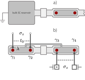
Figure 4: Grounded vs floating devices. (a) Switchable grounding of TI nanoribbon devices: By tuning the gate voltage applied to a local top gate at the narrowed section, the Josephson coupling energy $E_{J}$ between the TI nanoribbon and a grounded superconducting reservoir can be changed. As a consequence, one can switch between a grounded and a floating device. (b) Floating version of the device in Fig. 1. The two $s$-wave superconductors are connected by a superconducting bridge, i.e., the Majorana box is characterized by a single charging energy. Normal leads (vertical black lines) are tunnel-coupled to individual MBSs and amongst themselves by interference links to allow for interferometric readout of Pauli operators. The external boxes are symbolic for quantum dots or single-electron transistors which can be used to pump single electrons through the device and manipulate or read out qubit states. For details, see main text.

III.1 Floating vs grounded device

Braiding protocols for MBSs require switchable grounding of the host device Aasen2016 , i.e., the option to isolate the system against ground such that its finite capacitance defines an effective charging energy $E_{C}$. The principle is illustrated in Fig. 4(a), which differs from Fig. 1 in that the connector to ground is replaced by a superconducting reservoir coupled to the system via a narrow TI wire segment. As with the weak link in Sec. II, the geometric confinement implies that the connecting section is gapped and effectively realizes a tunnel junction. A top gate may be installed to tune the tunneling strength and, thereby, the Josephson energy $E_{J}$ between the superconducting regions connected by the junction. In this way, changes in the gate voltage effect a switch between floating (small $E_{J}$) and grounded (large $E_{J}$) configurations, see Ref. Aasen2016 for details.

The energy balance of a topological superconductor generally contains a charging energy, $E_{C}$, and a dimensionless backgate parameter $n_{g}$ Fu2010 ; Beri2012 ; Altland2013 ; Beri2013 controlling the energetically preferred charge on it. Here, $E_{C}$ relates to the electrostatic capacitance of those regions of the device that are in good electrical contact with each other. For instance, the floating device shown in Fig. 4(b) contains a superconducting bridge connecting its left and right half, and this leads to a ‘Majorana box’ characterized by a single charging energy. In general, the energy balance is influenced by both, Josephson coupling, $E_{J}$, to a bulk superconductor [as in Fig. 4(a)], and a charging energy, $E_{C}$, and the sum of these contributions,

$$H_{C}=E_{C}(2\hat{N}_{s}+\hat{n}_{\gamma}-n_{g})^{2}-E_{J}\cos\hat{\phi}_{s}$$ (16)

adds to the Hamiltonian $H_{\rm eff}$ in Eq. (15) Fu2010 ; Beri2012 ; Altland2013 ; Beri2013 . The number operator $\hat{N}_{s}$ is canonically conjugate to the phase difference between the superconductors, $\hat{\phi}_{s}$, and counts the number of Cooper pairs on the island, while $\hat{n}_{\gamma}=(i/2)[\gamma_{1}\gamma_{2}+\gamma_{3}\gamma_{4}]$ measures the fermion number in the Majorana sector. The Hamiltonian $H_{\rm eff}$ describes the low-energy sector of the system in that above-gap quasiparticles and surface states with $j\neq-1/2$ are not taken into account.

Externally imposed changes in the ratio $E_{J}/E_{C}$ may be applied to access Majorana fermion occupancies, e.g., via the parity-to-charge conversion protocol of Ref. Aasen2016 . For few-$\mu$m long nanowires, a typical charging energy is $E_{C}\approx 0.1$ K. We then expect a tunable parameter range of order $0.1\lesssim E_{J}/E_{C}\lesssim 10$. This tunability is of key importance to QIP protocols relying on the non-Abelian braiding statistics of MBSs Aasen2016 .

III.2 Majorana box qubit

We next consider the floating device (‘box’) shown in Fig. 4(b), where $E_{J}=0$ and a Majorana box qubit can be realized. For a long TI nanoribbon with exponentially small hybridization energy, $\varepsilon$, the four MBSs in Fig. 4(b) effectively represent zero-energy modes. On energy scales small against both $E_{C}$ and the proximity gap $\Delta$, and assuming that the backgate parameter $n_{g}$ is close to an integer value, charge quantization on the box implies that fermion parity is a good quantum number, $\gamma_{1}\gamma_{2}\gamma_{3}\gamma_{4}={\cal P}=\pm 1$. As a consequence, the Majorana box has a two-fold degenerate ground state. The different components of the corresponding emergent spin-$1/2$ operator are encoded by spatially separated Majorana operators. Specifically, we choose Pauli operators as Beri2012 ; Altland2013 ; Beri2013

$$\sigma_{x}=i\gamma_{3}\gamma_{1},\quad\quad\sigma_{y}=i\gamma_{2}\gamma_{3},\quad\sigma_{z}=i\gamma_{1}\gamma_{2}.$$ (17)

Equivalent representations follow from the parity constraint, e.g., $\sigma_{z}=-i{\cal P}\gamma_{3}\gamma_{4}$, see Fig. 4(b).

The degenerate two-level system defined in Eq. (17) can effectively encode arbitrary qubit states $|\psi\rangle=\alpha|0\rangle+\beta|1\rangle$ (with $\sigma_{z}|0\rangle=|0\rangle$ and $\sigma_{z}|1\rangle=-|1\rangle$). The option to address different Pauli operators via spatially non-local access operations in a topologically protected setting, cf. Sec. III.3, holds promise for a versatile and robust hardware qubit for QIP applications, see Refs. Landau2016 ; Plugge2016 ; Plugge2017 ; Karzig2017 . We expect that at temperatures of a few milli-Kelvin, above-gap quasiparticles will limit the qubit lifetime. Although further work would be required to quantify the expected time scales, we note that the mechanisms for decoherence (quasiparticle poisoning, in the first place) are similar to those in other topological Majorana qubits Aasen2016 ; Plugge2017 ; Karzig2017 ; Plugge2016 . In what follows, we consider protocols operating on shorter time scales where such detrimental effects can be neglected.

III.3 Basic quantum operations

By suitably designing the device, Pauli operators can be read out via interferometric conductance measurements Plugge2016 ; Plugge2017 . For the Majorana box qubit in Fig. 4(b), these measurements would require the coupling of a pair of MBSs to tunnel electrodes. For instance, the coupling to $\gamma_{1}$ and $\gamma_{2}$ would amount to addressing the Pauli operator $\sigma_{z}$ of Eq. (17). Consider these two access leads connected by an additional interference link of tunnel strength $t_{0}$ away from the device (‘reference arm’). Electron transport from lead $1\to 2$ can then either be (i) through the box, where the cotunneling amplitude is given by $it_{z}\gamma_{1}\gamma_{2}=t_{z}\sigma_{z}$ with $t_{z}\simeq\lambda^{2}/E_{C}$ for elementary tunnel amplitude $\lambda$, or (ii) through the reference arm with amplitude $t_{0}$. The tunnel conductance between leads 1 and 2 is thus given by

$$G_{12}=\frac{e^{2}}{h}\nu_{1}\nu_{2}|t_{0}+t_{z}\sigma|^{2},$$ (18)

where $\sigma=\pm$ refers to the eigenvalues of $\sigma_{z}$ and $\nu_{1,2}$ denotes the respective density of states in the normal leads. The outcome of the measurement depends on $\sigma$, and this means that the conductance measurement projects the original qubit state $|\psi\rangle=\alpha|0\rangle+\beta|1\rangle$ to the respective $\sigma_{z}$-eigenstate. With probability $|\alpha|^{2}$ ($|\beta|^{2}=1-|\alpha|^{2}$) the qubit assumes the state $|0\rangle$ ($|1\rangle$) after the measurement. Projective conductance measurements of this type may be applied to read out arbitrary Pauli operators or to initialize the qubit in a Pauli eigenstate. It is worth mentioning that for the device in Fig. 4(b), the Pauli operator $\sigma_{y}=i\gamma_{2}\gamma_{3}$ can be measured without an additional reference link shared by leads 2 and 3 since the central superconducting bridge already provides this link Karzig2017 .

The controlled manipulation of qubit states, $|\psi\rangle$, however, requires additional access elements. Specifically, the application of a given Pauli operator (17) to a state $|\psi\rangle$ can be realized through the pumping of a single electron between a pair of quantum dots (or single-electron transistors) tunnel-coupled to the MBSs corresponding to the operator Landau2016 ; Plugge2016 ; Plugge2017 . Here, the dots are assumed to be in the single-occupancy regime, where the respective energy levels can be changed by means of gate voltages. The pumping of a single electron from dot $1\to 2$ then implies a unitary state transformation, $|\psi\rangle\to U|\psi\rangle$, where $U$ corresponds to the respective Pauli operator. This transformation law is topologically robust in the sense that it is independent of details of the protocol Plugge2017 . For instance, it does not depend on the values of the tunnel couplings nor on the precise time dependence of gate voltages. However, it has to be made sure that the electron ends up in the desired final state, either by a confirmation measurement of the dot charge or by running the protocol in an adiabatically slow fashion. Finally, also pairs of dots may be connected by additional phase-coherent reference arms to effectively realize arbitrary single-qubit phase gates. However, in contrast to the Pauli operators discussed above, such phase gates generally are not topologically protected anymore due to measurement-induced dephasing processes, see Ref. Plugge2017 for details. The latter processes are essential for projective readout and/or initialization but are detrimental to manipulations of the qubit state.

Alternative proposals to read out, manipulate, or initialize Majorana box qubit states can be found in Refs. Plugge2017 ; Karzig2017 . For example, quantum dots may be applied as an alternative to leads for readout purposes. Furthermore, by measuring products of Pauli operators on different boxes, one may entangle the states of the corresponding qubits. In particular, a measurement-based protocol for generating a controlled-NOT gate can be found in Ref. Plugge2017 .

III.4 Discussion

We now turn to a critical discussion of the proposed platform. Since MBSs in the TI setup are formed from topological surface states, they can be expected to enjoy an intrinsic protection mechanism against both elastic impurity scattering and pair-breaking disorder. At the same time, presently available TI materials are not as clean as the corresponding semiconductor nanowire systems, and significant experimental progress will be needed to verify the practical usefulness of this platform. In what follows, we address the robustness of MBSs in TI nanoribbon devices against possibly detrimental mechanisms in view of the above results, and compare the TI implementation to alternative realizations.

First, it may be difficult to precisely tune the magnetic flux to $\varphi=1/2$ in the proximitized regions, even though one can adjust magnetic fields to high accuracy. Such a flux mismatch could arise because of (i) inhomogeneities in the cross section area, (ii) misalignment between the magnetic field and the TI nanoribbon axis which, in addition, weakly breaks rotation symmetry and therefore mixes $j=-1/2$ states with $j\neq-1/2$ high-energy states, and/or (iii) because different nanowire parts may not be exactly parallel to each other. For small flux mismatch, the topological energy gap appearing in Eq. (9) will change only slightly due to the corresponding change in $M(\varphi)$, see Eq. (10), without affecting the robustness of MBSs. However, one then needs a finite electrochemical potential $\mu_{S}=\mu(|z|>W/2)$ in the proximitized regions, in contrast to our assumption in Eq. (4). In particular, $M(\varphi)<|\mu_{S}|<\hbar v_{2}/R$ is required for well-defined helical 1D states when $\Delta=0$ (which then yield MBSs for $\Delta\neq 0$). We conclude that flux mismatch is not expected to create serious problems for the robustness of MBSs.

Second, we address what happens for finite electrochemical potential $\mu_{S}$ in the proximitized regions, where we focus on the case $\varphi=1/2$. Recalling that the $\Delta=0$ states with $j=-1/2$ have linear dispersion, we expect that a shift of $\mu_{S}$ enters physical quantities mainly through the difference $\mu-\mu_{S}$. In effect, the above $\mu_{S}=0$ results thus apply again.

Next we consider the localization length of MBSs in our setup and compare the result to other platforms. For the device in Fig. 1, different length scales govern the MBS decay into the inner and the outer part. Taking the proximity gap as $\Delta=0.18$ meV, one gets $\xi_{\Delta}=\hbar v_{1}/\Delta=1.25\leavevmode\nobreak\ \mu$m on the superconducting side, while the decay into the inner segment is governed by the much shorter length $\xi$ in Eq. (14). (The precise value of $\xi$ depends on the parameters $W,R_{0}/R,$ and $\mu$.) The MBS localization length is longer than $\xi_{\Delta}$ in semiconductor nanowires, where a typical spin-orbit coupling energy $\hbar\alpha\approx 20$ eV$\times$nm translates into the length scale $125\leavevmode\nobreak\$nm Sarma2012 . The above estimates indicate that one may need rather long proximitized TI nanowires (exceeding at least $5\leavevmode\nobreak\ \mu$m) in order to have negligible MBS overlap, e.g., between $\gamma_{1}$ and $\gamma_{2}$ in Fig. 4(b). While this requirement constitutes a slight disadvantage against semiconductor nanowires, we note that sufficiently long TI nanoribbons are already available Cho2015 ; Jauregui2016 . Similar values for the MBS localization length as found for the TI case above have also been estimated for the HgTe platform Deacon2017 ; Bocquillon2017 .

We continue by studying the maximum time scale $t_{0}$ on which the simplest type of Majorana qubit could be operated without dephasing for different platforms, using a device as in Fig. 1. In our TI setting, this scale is defined by $t^{-1}_{0}=\varepsilon(0)$, see Eq. (13). Indeed, for times $t>t_{0}$, the hybridization of the inner MBSs in Fig. 1 will inevitably dephase the qubit state. Clearly, it is then desirable to access time scales $t_{0}$ as long as possible. We observe from Eq. (14) that this condition is reached by choosing $\mu=0$ and a large width $W$ of the central segment, see Figs. 2 and 3. For instance, choosing $W=300$ nm and $|\mu|<0.2$ meV, we find $\varepsilon(0)<0.027\leavevmode\nobreak\ \mu$eV, and hence $t_{0}>2.4\leavevmode\nobreak\ \mu$s. This time scale exceeds the one estimated for semiconductor nanowires Aasen2016 . However, in practice an important additional limitation on operation times for Majorana qubits may come from quasiparticle poisoning. The poisoning time is known to be $\gtrsim 1\leavevmode\nobreak\ \mu$s for semiconductor Majorana devices Albrecht2016b but remains to be studied for proximitized TI systems.

As elaborated in Sec. I, semiconductor nanowires define the experimentally most advanced platform for Majorana states at present, and detailed proposals for Majorana qubits in that platform have appeared Vijay2016 ; Aasen2016 ; Plugge2017 ; Karzig2017 . Nonetheless, this implementation also has some drawbacks. As remarked before, the chemical potential has to be chosen close to the band bottom, which in turn renders states susceptible to the effects of disorder. Such problems could probably be avoided in a 2D architecture, where a 2D electron gas (2DEG) with strong spin-orbit coupling is proximitized by a lithographically patterned superconducting top layer Shabani2016 ; Hell2017 ; Pientka2017 . Nonetheless, the chemical potential window allowing for robust MBSs is arguably bigger for the TI nanoribbon case. Moreover, the implementation of Majorana box qubits in a semiconductor nanowire setting has encountered difficulties due to the need for separate reference links Marcus2017 . Using our TI nanoribbon setup (and similarly for 2DEG implementations), this problem can be avoided by designing reference links from the TI itself, see Figs. 4 and 5.

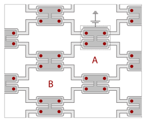
Figure 5: 2D network of Majorana box qubits using proximitized TI nanoribbons for implementing a Majorana surface code. Stabilizers of type A or B correspond to products of eight Majorana operators around a minimal plaquette as indicated. Access elements for initialization, manipulation, and readout of stabilizers are not shown but described in the main text.

IV Conclusions and outlook

In this paper, we have outlined how Majorana qubits can be defined and operated in a proximitized TI nanoribbon architecture. The key element of the construction are gate-tunable internal tunnel junctions realized through narrowed regions of lowered axial magnetic flux in TI nanoribbons. This allows us to tune the hybridization of MBSs emerging from a topologically protected helical 1D surface state mode, and thereby makes it possible to manipulate the quantum information. The linear dispersion of the 1D modes in this platform is expected to give the MBSs a high level of robustness. (In this regard, the situation may be better than in semiconductor wire platforms, where one is operating close to the bottom of a parabolic band.) We are confident that this platform is sufficiently versatile and flexible to implement the quantum information processing protocols outlined above.

Once proof-of-principle experiments have confirmed this expectation, one may envisage the extension of the system to 2D networks containing many Majorana box qubits. Specifically, the blueprint sketched in Fig. 5 indicates the extension to a network realizing a two-dimensional surface code, cf. Refs. Terhal2012 ; Vijay2015 ; Landau2016 ; Plugge2016 . The surface code approach builds on so-called stabilizer operators corresponding to products of eight Majorana operators surrounding the minimal plaquettes of Fig. 5. There are two types (A and B) of such operators, and the essence of the surface code is that all of them commute. The binary eigenvalues $\pm 1$ of the stabilizers then define the physical qubits of the system. During each operational cycle of the system the majority of these qubits is measured (‘stabilized’), and projection onto the highly entangled degenerate ground states of the system takes place. The few qubits exempt from the measurement process serve as logical qubits and can be manipulated along the lines of the discussion above.

In contrast to the ‘unfolded’ linearly arranged box qubit in Fig. 4(b), Fig. 5 suggests an alternative construction, where pairs of adjacent proximitized TI nanowires are connected through superconducting bridges to form 90-deg rotated ‘H’-type structures. Each of these structures represents a Majorana box with its own charging energy. Pairs of adjacent MBSs on neighboring boxes are connected by tunnel links as shown in Fig. 5. Since the TI nanoribbon network is most likely fabricated by lithographic and/or wet etching means, the present platform would naturally employ tunable TI nanoribbon parts for those tunnel links as well. In this way, the need for separate wires and/or other materials required by the corresponding semiconductor architecture Plugge2016 ; Plugge2017 ; Karzig2017 might be avoided. Since the proximitized TI nanoribbon parts in Fig. 5 are arranged parallel to each other, the MBSs can be generated simultaneously under a uniform applied magnetic field, provided the nanoribbon cross section can be accurately controlled in the fabrication process.

Appendix A Spinor wave functions

Here we provide the explicit form of the BdG eigenstates, $\Psi(z)$, for the device in Fig. 1. For notational simplicity, we employ units with $\hbar v_{1}=1$. Putting $j=-1/2$, since we are interested in constructing Majorana bound states, we consider only energies below the superconducting gap, $|E|<\Delta$. With $H_{\rm BdG}$ in Eq. (8), we shall first write down general solutions of the BdG equation in each of the three regions. These solutions are subsequently matched at the interface points $z=\pm W/2$ by continuity. Using parameters $A_{1,2}^{(\pm)}$, the solution for $|z|>W/2$ decaying at $|z|\to\infty$ reads

$$\Psi(z)\Bigr{|}_{|z|>W/2}=e^{-\sqrt{\Delta^{2}-E^{2}}|z|}\left[A^{(s)}_{1}\left(\begin{array}[]{c}E\\ -s\sqrt{\Delta^{2}-E^{2}}\\ 0\\ \Delta e^{is\phi/2}\end{array}\right)+A^{(s)}_{2}\left(\begin{array}[]{c}-s\sqrt{\Delta^{2}-E^{2}}\\ -E\\ \Delta e^{is\phi/2}\\ 0\end{array}\right)\right],\quad s={\rm sgn}(z)=\pm,$$ (19)

where the first and second (third and fourth) component refers to the spin structure of the particle (hole) part of the Nambu spinor. In the central region $|z|<W/2$, with coefficients $B^{(\pm)}_{1,2}$ the solution is given by

$$\Psi(z)\Bigr{|}_{|z|<W/2}=\sum_{\pm}\left[B^{(\pm)}_{1}e^{\pm\sqrt{M_{0}^{2}-(E+\mu)^{2}}z}\left(\begin{array}[]{c}\pm(M_{0}+E+\mu)\\ \sqrt{M_{0}^{2}-(E+\mu)^{2}}\\ 0\\ 0\end{array}\right)+B^{(\pm)}_{2}e^{\pm\sqrt{M_{0}^{2}-(E-\mu)^{2}}z}\left(\begin{array}[]{c}0\\ 0\\ \pm(M_{0}-E+\mu)\\ \sqrt{M_{0}^{2}-(E-\mu)^{2}}\end{array}\right)\right].$$ (20)

Imposing continuity at $z=\pm W/2$, we find that eigenenergies with $|E|<{\rm min}(\Delta,M_{0})$ follow from the zero-determinant condition in Eq. (11). The determinant $D(E)$ is a symmetric function of $E$ and given by

$$D(E) = -2\Delta^{2}a_{+}a_{-}\cos\phi+\sum_{\pm}\left[(2E^{2}-\Delta^{2})\left(a_{+}a_{-}\pm\mu^{2}\mp E^{2}\right)\pm M_{0}^{2}\Delta^{2}\right]\cosh[(a_{-}\pm a_{+})W]$$

$$+ 2E\sqrt{\Delta^{2}-E^{2}}\sum_{\pm}\left[(E-\mu)a_{+}\pm(E+\mu)a_{-}\right]\sinh[(a_{-}\pm a_{+})W],\quad a_{\pm}(E)\equiv\sqrt{M_{0}^{2}-(E\pm\mu)^{2}}.$$

References

- (1) M.Z. Hasan and C.L. Kane, Rev. Mod. Phys. 82, 3045 (2010).
- (2) X.L. Qi and S.C. Zhang, Rev. Mod. Phys. 83, 1057 (2011).
- (3) J. Alicea, Rep. Prog. Phys. 75, 076501 (2012).
- (4) M. Leijnse and K. Flensberg, Semicond. Sci. Techn. 27, 124003 (2012).
- (5) Y. Tanaka, M. Sato, and N. Nagaosa, J. Phys. Soc. Jpn. 81, 011013 (2012).
- (6) C.W.J. Beenakker, Annu. Rev. Con. Mat. Phys. 4, 113 (2013).
- (7) Y. Ando and L. Fu, Annu. Rev. Con. Mat. Phys. 6, 361 (2015).
- (8) M. Sato and Y. Ando, preprint arXiv:1608.03395.
- (9) C. Nayak, S.H. Simon, A. Stern, M. Freedman, and S. Das Sarma, Rev. Mod. Phys. 80, 1083 (2008).
- (10) L. Fu and C.L. Kane, Phys. Rev. Lett. 100, 096407 (2008).
- (11) J.D. Sau, S. Tewari, and S. Das Sarma, Phys. Rev. A 82, 052322 (2010).
- (12) J. Alicea, Y. Oreg, G. Refael, F. von Oppen, and M.P.A. Fisher, Nat. Phys. 7, 412 (2011).
- (13) D.J. Clarke, J.D. Sau, and S. Tewari, Phys. Rev. B 84, 035120 (2011).
- (14) T. Hyart, B. van Heck, I. C. Fulga, M. Burrello, A.R. Akhmerov, and C.W.J. Beenakker, Phys. Rev. B 88, 035121 (2013).
- (15) S. Vijay and L. Fu, Phys. Rev. B 94, 235446 (2016).
- (16) D. Aasen et al., Phys. Rev. X 6, 031016 (2016).
- (17) B. Béri and N.R. Cooper, Phys. Rev. Lett. 109, 156803 (2012).
- (18) A. Altland and R. Egger, Phys. Rev. Lett. 110, 196401 (2013).
- (19) B. Béri, Phys. Rev. Lett. 110, 216803 (2013).
- (20) S. Plugge, A. Rasmussen, R. Egger, and K. Flensberg, New J. Phys. 19, 012001 (2017).
- (21) T. Karzig et al., preprint arXiv:1610.05289.
- (22) B.M. Terhal, F. Hassler, and D.P. DiVincenzo, Phys. Rev. Lett. 108, 260504 (2012).
- (23) S. Vijay, T.H. Hsieh, and L. Fu, Phys. Rev. X 5, 041038 (2015).
- (24) L.A. Landau, S. Plugge, E. Sela, A. Altland, S.M. Albrecht, and R. Egger, Phys. Rev. Lett. 116, 050501 (2016).
- (25) S. Plugge, L.A. Landau, E. Sela, A. Altland, K. Flensberg, and R. Egger, Phys. Rev. B 94, 174514 (2016).
- (26) B.M. Terhal, Rev. Mod. Phys. 87, 307 (2015).
- (27) V. Mourik, K. Zuo, S.M. Frolov, S.R. Plissard, E.P.A. Bakkers, and L.P. Kouwenhoven, Science 336, 1003 (2012).
- (28) H. Zhang et al., preprint arXiv:1603.04069.
- (29) S.M. Albrecht, A.P. Higginbotham, M. Madsen, F. Kuemmeth, T.S. Jespersen, J. Nygård, P. Krogstrup, and C.M. Marcus, Nature 531, 206 (2016).
- (30) S.M. Albrecht, E.B. Hansen, A.P. Higginbotham, F. Kuemmeth, T.S. Jespersen, J. Nygård, P. Krogstrup, J. Danon, K. Flensberg, and C.M. Marcus, Phys. Rev. Lett. 118, 137701 (2017).
- (31) J. Wiedenmann et al., Nature Comm. 7, 10303 (2016).
- (32) E. Bocquillon, R.S. Deacon, J. Wiedemann, P. Leubner, T.N. Klapwijk, C. Brüne, K. Ishibashi, H. Buhmann, and L.W. Molenkamp, Nature Nanotech. 12, 137 (2017).
- (33) A.M. Cook and M. Franz, Phys. Rev. B 84, 201105 (2011).
- (34) A.M. Cook, M.M. Vazifeh, and M. Franz, Phys. Rev. B 86, 155431 (2012).
- (35) P. Sitthison and T.D. Stanescu, Phys. Rev. B 90, 035313 (2014).
- (36) F. de Juan, R. Ilan, and J.H. Bardarson, Phys. Rev. Lett. 113, 107003 (2014).
- (37) R. Ilan, J.H. Bardarson, H.-S. Sim, and J.E. Moore, New J. Phys. 16, 053007 (2014).
- (38) G.Y. Huang and H.Q. Xu, preprint arXiv:1612.02199.
- (39) S. Cho, B. Dellabetta, R. Zhong, J. Schneeloch, T. Liu, G. Gu, M.J. Gilbert, and N. Mason, Nature Comm. 6, 7634 (2015).
- (40) L.A. Jauregui, M.T. Pettes, L.P. Rokhinson, L. Shi, and Y.P. Chen, Nature Nanotech. 11, 345 (2016).
- (41) P.M. Ostrovsky, I.V. Gornyi, and A.D. Mirlin, Phys. Rev. Lett. 105, 036803 (2010).
- (42) Y. Zhang and A. Vishwanath, Phys. Rev. Lett. 105, 206601 (2010)
- (43) J. H. Bardarson, P.W. Brouwer, and J. E. Moore, Phys. Rev. Lett. 105, 156803 (2010).
- (44) R. Egger, A. Zazunov, and A.L. Yeyati, Phys. Rev. Lett. 105, 136403 (2010).
- (45) A. Kundu, A. Zazunov, A.L. Yeyati, T. Martin, and R. Egger, Phys. Rev. B 83, 125429 (2011).
- (46) J.H. Bardarson and J.E. Moore, Rep. Prog. Phys. 76, 056501 (2013).
- (47) Although the infinite proximitized TI nanoribbon with belongs to the time reversal invariant symmetry class III and Kramers pairs of degenerate Majorana states should be expected, the non-quantized magnetic flux felt at the wire ends breaks time reversal, and lifts Kramers degeneracy, see Ref. Cook2012 for a detailed discussion.
- (48) L. Fu, Phys. Rev. Lett. 104, 056402 (2010).
- (49) R. Hützen, A. Zazunov, B. Braunecker, A.L. Yeyati, and R. Egger, Phys. Rev. Lett. 109, 166403 (2012).
- (50) M.J. Biercuk, D.J. Reilly, T.M. Buehler, V.C. Chan, J.M. Chow, R.G. Clark, and C.M. Marcus, Phys. Rev. B 73, 201402(R) (2006).
- (51) S. Das Sarma, J.D. Sau, and T.D. Stanescu, Phys. Rev. B 86, 220506(R) (2012).
- (52) J. Shabani et al., Phys. Rev. B 93, 155402 (2016).
- (53) M. Hell, M. Leijnse, and K. Flensberg, Phys. Rev. Lett. 118, 107701 (2017).
- (54) F. Pientka, E. Berg, A. Yacoby, A. Stern, and B.I. Halperin, preprint arXiv:1609.09482.
- (55) H.J. Suominen, M. Kjaergaard, A.R. Hamilton, J. Shabani, C.J. Palmstrøm, C.M. Marcus, and F. Nichele, arXiv:1703.03699.