Super Generalized Central Limit Theorem
–Limit distributions for sums of non-identical random variables with power-laws–

Abstract

In nature or societies, the power-law is present ubiquitously, and then it is important to investigate the characteristics of power-laws in the recent era of big data. In this paper we prove the superposition of non-identical stochastic processes with power-laws converges in density to a unique stable distribution. This property can be used to explain the universality of stable laws such that the sums of the logarithmic return of non-identical stock price fluctuations follow stable distributions.

Introduction—.There are a lot of data that follow the power-laws in the world. Examples of recent studies include, but are not limited to the financial market mandelbrot1997variation ; mantegna1994stochastic ; mantegna1995scaling ; gopikrishnan1998inverse ; gabaix2006institutional ; denys2016universality ; tanaka2016statistical , the distribution of people’s assets druagulescu2001exponential , the distribution of waiting times between earthquakes occurring bak2002unified and the dependence of the number of wars on its intensity roberts1998fractality . It is then important to investigate the general characteristics of power-laws.

In particular, as for the data in the financial market, Mandelbrot mandelbrot1997variation firstly argued that the distribution of the price fluctuations of cotton follows a stable law. Since the 1990’s, there has been a controversy as to whether the central limit theorem or the generalized central limit theorem (GCLT) Kolmogorov as sums of power-law distributions can be applied to the data of the logarithmic return of stock price fluctuations. In particular, Mantegna and Stanley argued that the logarithmic return follows a stable distribution with the power-law index $\alpha<2$ mantegna1994stochastic ; mantegna1995scaling , and later they denied their own argument by introducing the cubic laws ($\alpha=3$) gopikrishnan1998inverse . Even recently, some researchers gabaix2006institutional ; denys2016universality ; tanaka2016statistical have argued whether a distribution of the logarithmic returns follows power-laws with $\alpha>2$ or stable laws with $\alpha<2$. On the other hand, it is necessary to prepare very large data sets to elucidate true tail behavior of distributions weron2001levy . In this respect, the recent study tanaka2016statistical showed that the large and high-frequency arrowhead data of the Tokyo stock exchange (TSE) support stable laws with $1<\alpha<2$.

In this study, we show that the sums of the logarithmic return of multiple stock price fluctuations follows stable laws, and it can be described from a theoretical background. We will extend the GCLT to sums of independent non-identical stochastic processes. We call this Super Generalized Central Limit Theorem (SGCLT).

Summary of stable distributions and the GCLT—.A probability density function $S(x;\alpha,\beta,\gamma,\mu)$ of random variable $X$ following a stable distribution nolan2003stable is defined with its characteristic function $\phi(t)$ as:

$$S(x;\alpha,\beta,\gamma,\mu)=\frac{1}{2\pi}\int_{-\infty}^{\infty}\phi(t)e^{-ixt}{\rm d}x,$$

where $\phi(t;\alpha,\beta,\gamma,\mu)$ is expressed as:

$$\phi(t)=\exp{\{i\mu t-\gamma^{\alpha}|t|^{\alpha}(1-i\beta{\rm sgn}(t)w(\alpha,t))\}}$$

$$w(\alpha,t)=\left\{\begin{aligned} &\tan\left(\pi\alpha/2\right)&\text{if}&\ \ \alpha\neq 1\\ &-2/\pi\log|t|&\text{if}&\ \ \alpha=1.\end{aligned}\right.$$

The parameters $\alpha,\beta,\gamma$ and $\mu$ are real constants satisfying $0<\alpha\leq 2$, $-1\leq\beta\leq 1$, $\gamma>0$, and denote the indices for power-law in stable distributions, the skewness, the scale parameter and the location, respectively. When $\alpha=2$ and $\beta=0$, the probability density function obeys a normal distribution. Note that explicit forms of stable distributions are not known for general parameters $\alpha$ and $\beta$ except for a few cases such as the Cauchy distribution ($\alpha=1,\beta=0$).

A stable random variable satisfies the following property for the scale and the location parameters. A random variable $X$ follows $S(\alpha,\beta,\gamma,\mu)$, when

$$X\overset{d}{=}\left\{\begin{aligned} &\gamma X_{0}+\mu&\ \text{if}&\ \ \alpha\neq 1\\ &\gamma X_{0}+\mu+\frac{2}{\pi}\beta\gamma\ln\gamma&\ \text{if}&\ \ \alpha=1,\end{aligned}\right.$$ (1)

where $X_{0}=S(\alpha,\beta,1,0)$. When the random variables $X_{j}$ satisfy $X_{j}\sim S(x;\alpha,\beta_{j},\gamma_{j},0)$, the superposition $Z_{n}=(X_{1}+\cdots+X_{n})/n^{\frac{1}{\alpha}}$ of independent random variables $\{X_{j}\}_{j=1,\cdots,n}$ that have different parameters except for $\alpha$ is also in the stable distribution family as:

$$Z_{n}\sim S(\alpha,\hat{\beta},\hat{\gamma},\hat{\mu}),$$ (2)

where the parameters $\hat{\beta},\hat{\gamma}$ and $\hat{\mu}$ are expressed as:

$$\displaystyle\hat{\beta}=\frac{\sum_{j=1}^{n}\beta_{j}\gamma_{j}^{\alpha}}{\sum_{j=1}^{n}\gamma_{j}^{\alpha}},\hat{\gamma}=\left\{\frac{\sum_{j=1}^{n}\gamma_{j}^{\alpha}}{n}\right\}^{\frac{1}{\alpha}}\ \text{and}$$

$$\hat{\mu}=\left\{\begin{array}[]{lll}0&\text{if}&\alpha\neq 1\\ -\frac{2\ln n}{n\pi}\sum_{j=1}^{n}\beta_{j}\gamma_{j}&\text{if}&\alpha=1.\end{array}\right.$$

We can prove this immediately by the use of the characteristic function for the sums of random variables expressed as the product of their characteristic functions:

$$\phi(t;\alpha,\hat{\beta},\hat{\gamma},\hat{\mu})=\prod_{j=1}^{n}\phi\left(t/n^{\frac{1}{\alpha}};\alpha,\beta_{j},\gamma_{j},0\right).$$

We focus on the GCLT. Let $f$ of $x$ be a probability density function of a random variable $X$ for $0<\alpha<2$:

$$f(x)\simeq\left\{\begin{aligned} &c_{+}x^{-(\alpha+1)}&\text{for}&\ \ x\to\infty\\ &c_{-}|x|^{-(\alpha+1)}&\text{for}&\ \ x\to-\infty,\end{aligned}\right.$$ (4)

with $c_{+},c_{-}>0$ being real constants. Then, according to the GCLT Kolmogorov , the superposition of independent, identically distributed random variables $X_{1},\cdots,X_{n}$ converges in density to a unique stable distribution $S(x;\alpha,\beta,\gamma,0)$ for $n\to\infty$, that is

$$\begin{split}Y_{n}&=\frac{\sum_{i=1}^{n}X_{i}-A_{n}}{n^{\frac{1}{\alpha}}}\xrightarrow{d}S(\alpha,\beta,\gamma,0)\ \text{for}\ n\to\infty,\\ A_{n}&=\left\{\begin{aligned} &0&\text{if}&\ \ 0<\alpha<1\\ &n^{2}\Im\ln(\varphi_{X}\left(1/n\right))&\text{if}&\ \ \alpha=1\\ &n\mathbb{E}[X]&\text{if}&\ \ 1<\alpha<2,\end{aligned}\right.\end{split}$$ (5)

where $\varphi_{X}$ is a characteristic function of $X$ as the expected value of $\exp(itX)$, $\mathbb{E}[X]$ is the expectation value of $X$, $\Im$ is an imaginary part of the argument, and parameters $\beta$ and $\gamma$ are expressed as:

$$\beta = \frac{c_{+}-c_{-}}{c_{+}+c_{-}},\ \gamma=\left\{\frac{\pi(c_{+}+c_{-})}{2\alpha\sin(\frac{\pi\alpha}{2})\Gamma(\alpha)}\right\}^{\frac{1}{\alpha}},$$

with $\Gamma$ being the Gamma function. When $\alpha=2$, we obtain $\mu=\int xf(x){\rm d}x$, $\sigma^{2}=\int x^{2}f(x){\rm d}x$ and the superposition $Y_{n}$ of the independent, identically distributed random variables converges in density to a normal distribution:

$$Y_{n} = \frac{\sum_{i=1}^{n}X_{i}-n\mu}{\sqrt{n}\sigma}\xrightarrow{d}\mathcal{N}(0,1),\ \text{for}\ n\to\infty.$$

Our generalization—.We consider an extension of this existing theorem for sums of non-identical random variables. In what follows we assume that the random variables $\{X_{i}\}_{i=1,\cdots,n}$ satisfy the following two conditions.

(Condition 1): The random variables $C_{+}>0$, $C_{-}>0$ obey respectively the distributions ${\rm P}_{c_{+}}(c)$, ${\rm P}_{c_{-}}(c)$, and satisfy $\mathbb{E}[C_{+}]<\infty$, $\mathbb{E}[C_{-}]<\infty$.

(Condition 2): The probability distribution function $f_{i}(x)$ of the random variables $X_{i}$ satisfies in $0<\alpha<2$:

$$f_{i}(x)\simeq\left\{\begin{aligned} &c_{+i}x^{-(\alpha+1)}&\text{for}&\ \ x\to\infty\\ &c_{-i}|x|^{-(\alpha+1)}&\text{for}&\ \ x\to-\infty,\end{aligned}\right.$$ (6)

where $c_{+i}$ and $c_{-i}$ are samples obtained by $C_{+}$ and $C_{-}$. We emphasize that the probability distribution function may not be obtained even when we integrate $f_{i}(x)$ over $c_{+i}$ and $c_{-i}$.

The main claim of this paper is the following generalization of GCLT: The following superposition $S_{n}$ of non-identical random variables with power-laws converges in density to a unique stable distribution $S(x;\alpha,\beta^{*},\gamma^{*},0)$ for $n\to\infty$, where

$$\begin{aligned} S_{n}&=\frac{\sum_{i=1}^{n}X_{i}-A_{n}}{n^{\frac{1}{\alpha}}}\xrightarrow{d}S(x;\alpha,\beta^{*},\gamma^{*},0)\ \ \text{for}\ n\to\infty,\\ A_{n}&=\left\{\begin{array}[]{lll}0&\text{if}&\ 0<\alpha<1\\ n\sum_{i=1}^{n}\Im\ln(\varphi_{i}\left(1/n\right))&\text{if}&\ \alpha=1\\ \sum_{i=1}^{n}\mathbb{E}[X_{i}]&\text{if}&\ 1<\alpha<2,\end{array}\right.\end{aligned}$$ (7)

with $\varphi_{i}$ being a characteristic function of $X_{i}$ as the expected value of $\exp(itX_{i})$, and parameters $\beta^{*},\gamma^{*},\beta_{i},\gamma_{i}$ are expressed as:

$$\beta^{*} = \frac{{\rm E}_{C_{+},C_{-}}[\beta_{i}\gamma_{i}^{\alpha}]}{{\rm E}_{C_{+},C_{-}}[\gamma_{i}^{\alpha}]},\ \ \gamma^{*}=\left\{{\rm E}_{C_{+},C_{-}}[\gamma_{i}^{\alpha}]\right\}^{\frac{1}{\alpha}},$$

$$\beta_{i} = \frac{c_{+i}-c_{-i}}{c_{+i}+c_{-i}},\ \ \gamma_{i}=\left\{\frac{\pi(c_{+i}+c_{-i})}{2\alpha\sin(\frac{\pi\alpha}{2})\Gamma(\alpha)}\right\}^{\frac{1}{\alpha}}.$$

Here ${\rm E}_{C_{+},C_{-}}[X]$ denotes the expectation value of $X$ with respect to random parameter distributions ${\rm P}_{c_{+}}$ and ${\rm P}_{c_{-}}$.

Proof—.Although the following is not mathematically rigorous, we give the following intuitive proof.

The probability distribution function of random variables $\{X_{j}\}_{j=1,\cdots,N}$ satisfying the Conditions 1-2 is expressed as:

$$f_{j}(x)\simeq\left\{\begin{aligned} &c_{+j}x^{-(\alpha+1)}&\text{for}&\ x\to+\infty\\ &c_{-j}|x|^{-(\alpha+1)}&\text{for}&\ x\to-\infty,\end{aligned}\right.$$

where $c_{+j}>0$ and $c_{-j}>0$ satisfy $\mathbb{E}[C_{+}]>0$ and $\mathbb{E}[C_{-}]>0$. The superposition $S_{N}$ is then defined as:

$$\begin{split}S_{N}&=\frac{\sum_{j=1}^{N}X_{j}-A_{N}}{N^{\frac{1}{\alpha}}},\\ A_{N}&=\left\{\begin{array}[]{lll}0&\text{if}&\ 0<\alpha<1\\ N\sum_{j=1}^{N}\Im\ln(\varphi_{j}\left(1/N\right))&\text{if}&\ \alpha=1\\ \sum_{j=1}^{N}\mathbb{E}[X_{j}]&\text{if}&\ 1<\alpha<2,\end{array}\right.\end{split}$$

where $\varphi_{j}$ is a characteristic function of $X_{j}$. On the other hand, let $N^{\prime}$ be $M\times N$ with some $M$, and $\{X_{ij}\}_{i=1,\cdots,M,j=1,\cdots,N}$ be samples given by the same parent to $X_{j}$ for each $j$. Then $\{X_{ij}\}_{i=1,\cdots,M,j=1,\cdots,N}$ are independent, identically distributed for $i=1,\cdots,M$ at a fixed index $j$. Then, we define the superposition $S_{N^{\prime}}$ as follows:

$$\begin{aligned} &S_{N^{\prime}}=\frac{\sum_{i=1}^{M}\sum_{j=1}^{N}X_{ij}-A_{N^{\prime}}}{N^{\prime\frac{1}{\alpha}}},\\ A_{N^{\prime}}&=\left\{\begin{array}[]{lll}0&\text{if}&\ 0<\alpha<1\\ M^{2}N\sum_{j=1}^{N}\left(\Im\ln(\varphi_{j}\left(1/(MN))\right)\right)&\text{if}&\ \alpha=1\\ M\sum_{j=1}^{N}\mathbb{E}[X_{j}]&\text{if}&\ 1<\alpha<2.\end{array}\right.\end{aligned}$$

Here, we do not consider the convergence of $S_{N}$ in density for $N\to\infty$, but consider the superposition $S_{N^{\prime}}$ for $N^{\prime}\to\infty$, since the superposition $S_{N}$ will converge to the same limiting distribution of $S_{N^{\prime}}$ if $S_{N}$ converges in density.

We focus on the convergence in density of $S_{N^{\prime}}$ for $M\to\infty$ and $N\to\infty$ as follows. About the previous $A_{N^{\prime}}$ in $S_{N^{\prime}}$, we express it as $A_{N^{\prime}}=\sum_{j=1}^{N}A_{M_{j}}$ with the following $A_{M_{j}}(j=1,\cdots,N)$,

$$A_{M_{j}} = \left\{\begin{aligned} &0&\text{if}&\ \ 0<\alpha<1\\ &M^{2}N\Im\ln(\varphi_{j}\left(1/MN\right))&\text{if}&\ \ \alpha=1\\ &M\mathbb{E}[X_{j}]&\text{if}&\ \ 1<\alpha<2.\end{aligned}\right.$$

Here, the superposition $S_{N^{\prime}}$ is described as:

$$S_{N^{\prime}} = \frac{\sum_{i=1}^{M}\sum_{j=1}^{N}X_{ij}-A_{N^{\prime}}}{N^{\prime\frac{1}{\alpha}}}$$

$$= \frac{\frac{\sum_{i=1}^{M}X_{i1}-A_{M_{1}}}{M^{\frac{1}{\alpha}}}+\cdots+\frac{\sum_{i=1}^{M}X_{iN}-A_{M_{N}}}{M^{\frac{1}{\alpha}}}}{N^{\frac{1}{\alpha}}}.$$

When $\alpha\neq 1$, let $Y_{M_{j}}$ be the superposition $\left(\sum_{i=1}^{M}X_{ij}-A_{M_{j}}\right)/{M^{\frac{1}{\alpha}}}$. Then, $Y_{M_{j}}$ converges in density to $S(\alpha,\beta_{j},\gamma_{j},0)$ for $M\to\infty$ according to the GCLT (5), that is

$$Y_{M_{j}}=\frac{\sum_{i=1}^{M}X_{ij}-A_{M_{j}}}{M^{\frac{1}{\alpha}}}\overset{d}{\to}S(\alpha,\beta_{j},\gamma_{j},0)\ \text{for}\ M\to\infty,$$

where $\beta_{j}$ and $\gamma_{j}$ are

$$\beta_{j} = \frac{c_{+j}-c_{-j}}{c_{+j}+c_{-j}},\ \gamma_{j}=\left\{\frac{\pi(c_{+j}+c_{-j})}{2\alpha\sin(\frac{\pi\alpha}{2})\Gamma(\alpha)}\right\}^{\frac{1}{\alpha}}.$$

Thus, with the stable property (2), we obtain the convergence of the superposition $S_{N^{\prime}}$ as follows:

$$S_{N^{\prime}} = \frac{\sum_{j=1}^{N}Y_{M_{j}}}{N^{\frac{1}{\alpha}}}$$

$$\overset{d}{\to} \frac{\sum_{j=1}^{N}Y_{j}}{N^{\frac{1}{\alpha}}}\ \ \text{for}\ M\to\infty,(Y_{j}\sim S(\alpha,\beta_{j},\gamma_{j},0))$$

$$\overset{d}{\to} S(x;\alpha,\beta^{*},\gamma^{*},0)\ \ \text{for}\ N\to\infty,$$

where $\beta^{*}$ and $\gamma^{*}$ are:

$$\beta^{*} = \lim_{N\to\infty}\frac{\sum_{j=1}^{N}\beta_{j}\gamma_{j}^{\alpha}}{\sum_{j=1}^{N}\gamma_{j}^{\alpha}}$$

$$= \lim_{N\to\infty}\frac{\frac{1}{N}\sum_{j=1}^{N}\beta_{j}\gamma_{j}^{\alpha}}{\frac{1}{N}\sum_{j=1}^{N}\gamma_{j}^{\alpha}}=\frac{{\rm E}_{C_{+},C_{-}}[\beta_{j}\gamma_{j}^{\alpha}]}{{\rm E}_{C_{+},C_{-}}[\gamma_{j}^{\alpha}]},$$

$$\gamma^{*} = \lim_{N\to\infty}\left\{\frac{\sum_{j=1}^{N}\gamma_{j}^{\alpha}}{N}\right\}^{\frac{1}{\alpha}}=\left\{{\rm E}_{C_{+},C_{-}}[\gamma_{j}^{\alpha}]\right\}^{\frac{1}{\alpha}}.$$

This proves the superposition $S_{N^{\prime}}$ converges in density to $S(\alpha,\beta^{*},\gamma^{*},0)$. Figure LABEL:fig:concept illustrates the concept of this proof.

As above, the superposition $S_{N^{\prime}}$ of non-identical stochastic processes converges in density to a unique stable distribution. Since the limiting distribution of $S_{N^{\prime}}$ is the same as that of $S_{N}$, $S_{N}$ also converges to $S(x,\alpha,\beta^{*},\gamma^{*},0)$. When $\alpha=1$, this statement does not hold because of dependence between $M$ and $N$ in $A_{M_{j}}$, but we find that the limit distribution of the superposition $S_{N}$ generally converges in density to $S(x;\alpha,\beta^{*},\gamma^{*},0)$ as can be seen in the following numerical examples.

Numerical confirmation—.As below, we confirm the claim of SGCLT (7) by some numerical experiments.

To verify the main claim numerically, we use two kinds of test: two-samples Kolmogorov-Smirnov (KS) test stephens1974edf and two-samples Anderson-Darling (AD) test anderson1952asymptotic with 5% significance level. We generate two data by different methods, and see the $P{-}values$ of both of tests. Then, unless the null hypothesis is rejected, we judge the two data follow the same distribution.

For the first data, we generate non-identical stochastic processes satisfying Conditions 1-2, and prepare the superposition obtained in the same way as (7). For the second data, we generate the random numbers that follow the stable distribution, where the first data will converge to the stable distribution according to (7). Note that we compare the superposition with not a cumulative distribution function but random numbers obtained from another numerical method described below since a cumulative distribution function of a stable distribution cannot be expressed explicitly except for a few cases.

For the first data, let us consider the chaotic dynamical system $x_{n+1}=g(x_{n})$, where $g(x)$ is defined umeno1998superposition as follows for $0<\alpha<2$:

$$g(x)=\left\{\begin{array}[]{lll}\frac{1}{\delta_{1}^{2}|x|}\left(\frac{|\delta_{1}x|^{2\alpha}-1}{2}\right)^{1/\alpha}&\text{for}&\ \ x>\frac{1}{\delta_{1}}\\ -\frac{1}{\delta_{1}\delta_{2}|x|}\left(\frac{1-|\delta_{1}x|^{2\alpha}}{2}\right)^{1/\alpha}&\text{for}&\ \ 0<x<\frac{1}{\delta_{1}}\\ \frac{1}{\delta_{1}\delta_{2}|x|}\left(\frac{1-|\delta_{2}x|^{2\alpha}}{2}\right)^{1/\alpha}&\text{for}&\ \ -\frac{1}{\delta_{2}}<x<0\\ -\frac{1}{\delta_{2}^{2}|x|}\left(\frac{|\delta_{2}x|^{2\alpha}-1}{2}\right)^{1/\alpha}&\text{for}&\ \ x<-\frac{1}{\delta_{2}}.\end{array}\right.$$

This mapping has a mixing property and an ergodic invariant density for almost all initial points $x_{0}$. One of the authors (KU) obtained the following explicit asymmetric power-law distribution as an invariant density umeno1998superposition :

$$\rho_{\alpha,\delta_{1},\delta_{2}}(x)=\left\{\begin{aligned} &\frac{\alpha\delta_{1}^{\alpha}x^{\alpha-1}}{\pi(1+\delta_{1}^{2\alpha}x^{2\alpha})}&\text{if}&\ \ x\geq 0\\ &\frac{\alpha\delta_{2}^{\alpha}|x|^{\alpha-1}}{\pi(1+\delta_{2}^{2\alpha}|x|^{2\alpha})}&\text{if}&\ \ x<0.\end{aligned}\right.$$

This asymmetric distribution behaves as follows for $x\to\pm\infty$:

$$\rho_{\alpha,\delta_{1},\delta_{2}}(x)\simeq\left\{\begin{aligned} &\frac{\alpha}{\pi\delta_{1}^{\alpha}}x^{-(\alpha+1)}&\text{for}&\ \ x\to+\infty\\ &\frac{\alpha}{\pi\delta_{2}^{\alpha}}|x|^{-(\alpha+1)}&\text{for}&\ \ x\to-\infty.\end{aligned}\right.$$

This is exactly the same expression with the condition of GCLT (4) for random variables in $X$. Then, putting the variables $\delta_{1}$ and $\delta_{2}$ be distributed, we can obtain various different distributions with the same power-laws.

We regard the parameters $\delta_{1i}$ and $\delta_{2i}$ as random samples obtained from $\Delta_{1}$ and $\Delta_{2}$, where $\Delta_{1}$ and $\Delta_{2}$ obey ${\rm P}_{\delta_{1}}(\delta)$ and ${\rm P}_{\delta_{2}}(\delta)$, respectively. These are defined for $\delta>0$ with finite mean.

Then the parameters $c_{+i}$ and $c_{-i}$ are given as $c_{+i}=\frac{\alpha}{\pi\delta_{1i}^{\alpha}}$ and $c_{-i}=\frac{\alpha}{\pi\delta_{2i}^{\alpha}}$, and $\mathbb{E}[C_{+}]<\infty$, $\mathbb{E}[C_{-}]<\infty$ are also satisfied since $\delta_{1i},\delta_{2i}$ are not 0 and samples from some random variables $\Delta_{1}$ and $\Delta_{2}$ with finite mean. As above, we can get some stochastic processes satisfying the Conditions 1-2.

For the second data, the random numbers generated with the following procedure follow a stable distribution chambers1976method . Let $\Theta$ and $\Omega$ be independent random numbers: $\Theta$ uniformly distributed in $\left(-\frac{\pi}{2},\frac{\pi}{2}\right)$, $\Omega$ exponentially distributed with mean $1$. In addition, let $R$ be as follows:

$$R=\left\{\begin{matrix}\frac{\sin\left(\alpha(\theta_{0}+\Theta)\right)}{(\cos\left(\alpha\theta_{0}\right)\cos\Theta)^{1/\alpha}}\left[\frac{\cos((\alpha-1)\Theta)}{\Omega}\right]^{(1-\alpha)/\alpha}&(\alpha\neq 1)\\ \frac{2}{\pi}\left[(\frac{\pi}{2}+\beta\Theta)\tan\Theta-\beta\log\left(\frac{\frac{\pi}{2}\Omega\cos\Theta}{\frac{\pi}{2}+\beta\Theta}\right)\right]&(\alpha=1),\end{matrix}\right.$$

for $0<\alpha\leq 2$ where $\theta_{0}=\arctan(\beta\tan(\pi\alpha/2))$. Then it follows that $R\sim S(x;\alpha,\beta,1,0)$. We get arbitrary stable distributions by the use of the property (1) about the scale parameter and the location.

$\alpha$	${\rm P}_{\delta_{1}}(\delta)$	${\rm P}_{\delta_{2}}(\delta)$	$N$	$L$	$P{-}value$ (KS test)	$P{-}value$ (AD test)
$0.5$	$1$(const)	$1$(const)	10000	50000	0.122	0.074
	${\rm U}(1,2)$	${\rm U}(1,2)$	1000	100000	0.561	0.413
	${\rm U}(0.5,1)$	${\rm U}(1,2)$	1000	100000	0.865	0.546
$1$	$1$	$1$	1000	100000	0.226	0.308
	${\rm U}(1,2)$	${\rm U}(1,2)$	1000	100000	0.741	0.497
	${\rm U}(0.5,1)$	${\rm U}(1,2)$	1000	100000	0.659	0.301
$1.5$	$1$	$1$	1000	100000	0.916	0.529
	${\rm U}(1,1.2)$	${\rm U}(1,1.2)$	10000	20000	0.768	0.548
	${\rm U}(0.5,1)$	${\rm U}(1.5,2)$	10000	30000	0.108	0.099

Table 1: $P-values$ of two tests

$\alpha$	${\rm P}_{\delta_{1}}(\delta)$	${\rm P}_{\delta_{2}}(\delta)$	random variables	N	L	KS test	AD test
$0.5$	3	1	$X_{i}-i/N$	2000	10000	0.136	0.110
	3	1	$X_{i}-\ \text{Crand}(0,1)$	1000	10000	0.289	0.190
$1$	3	1	$X_{i}-i/N$	1000	10000	0.305	0.081
	3	1	$X_{i}-\ \text{Crand}(0,1)$	2000	10000	0.145	0.093
$1.5$	3	1	$X_{i}-\ \text{Crand}(0,1)$	1000	10000	0.371	0.286

Table 2: $P-values$ of two tests

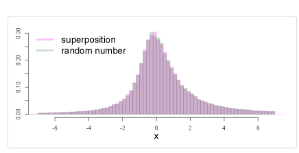
Figure 2: Comparison of two probability densities: the superposition ($N=10^{3}$, $L=10^{5}$ for $\alpha{=}1,\Delta_{1}{\sim}{\rm U}(0.5,1),\Delta_{2}{\sim}{\rm U}(1,2)$) and a stable distribution ($L=10^{5}$ for $\alpha{=}1,\beta^{*}{=}1/3,\gamma^{*}{=}1$)

With two data obtained accordingly, we see whether the superposition $S_{N}=(\sum_{i=1}^{N}X_{i}-A_{N})/N^{1/\alpha}$ numerically converges in density to a stable distribution $S(x;\alpha,\beta^{*},\gamma^{*},0)$ or not. Table 1 and 2 show $P{-}values$ of the KS test and the AD test for each $\alpha,\Delta_{1},\Delta_{2}$. The constant $L$ is the length of the sequence and $N$ is the number of sequences used for the superposition. The meaning of ${\rm U}(a,b)$ is the uniform distribution in $(a,b)$. Figure 2 illustrates an example of correspondence when $\alpha=1$. “Crand$(0,1)$” is the random numbers follow the standard Cauchy distribution. This case shows that the integral average of the probability distribution function with the Cauchy distribution is not uniquely determined.

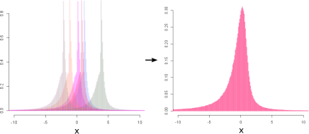
Figure 3: Image of the convergence process: The left figure shows some samples of random variables $X_{i}-\text{Crand}(0,1)$, where $\alpha=1,\delta_{1}=3,\delta_{2}=1$. The integration of them does not have an explicit expression because of the indefinite mean of the Cauchy distribution. However the sum (the right figure) converges to the $S(1,-0.5,2/3,0)$.

As can be seen from Table 1 and 2, we cannot reject the null hypothesis in any case for $\alpha$. In other words, the distribution of superposition $S_{N}$ and the stable distribution $S(x;\alpha,\beta^{*},\gamma^{*},0)$ are close enough in density according to our SGCLT.

In Figure 3, we can see that the superposition of non-identical distributed random variables converges.

Conclusions—.We have further generalized the GCLT for the sums of independent non-identical stochastic processes with the same power-law index $\alpha$. Our main claim of SGCLT can have more general applications since the various type of different power-laws exist in nature. Thus, our SGCLT can support the argument on the ubiquitous nature of stable laws such that the logarithmic return of the multiple stock price fluctuations follow a stable distribution with $1<\alpha<2$ by regarding them as the sums of non-identical random variables with power-laws. Take the data of the stock market as an example. Then, for the case that the distribution of the logarithmic return of each stock price fluctuation have the almost same power-law exponents and different scale parameters $(c_{+},c_{-})$, we get some trends or indicators according to this SGCLT.

The authors thank Dr. Shin-itiro Goto (Kyoto University) for stimulating discussions.

References

(1)
B. Mandelbrot, Journal of Business, 36, 394 (1963)
(2)
R. N. Mantegna, H. E. Stanley, Phys. Rev. Lett. 73, 2946
(1994)
(3)
R. N. Mantegna, H. E. Stanley, Nature, 376, 46 (1995)
(4)
P. Gopikrishnana, M. Meyer, L. A. N. Amaral, H.E. Stanley,
Eur. Phys. J. B, 3, 139 (1998)
(5)
X. Gabaix, P. Gopikrishnan, V. Plerou, H. E. Stanley, The
Quarterly Journal of Economics, 121, 2, 461 (2006)
(6)
M. Denys, T. Gubiec, R. Kutner, M. Jagielski, H. E. Stanley,
Phys. Rev. E, 94, 042305 (2016)
(7)
M. Tanaka, IEICE Technical Report, 116, 27 (2016) (In
Japanese)
(8)
A. Drgulescu, V. M. Yakovenko, Physica A:
Statistical Mechanics and its Applications, 299, 213
(2001)
(9)
P. Bak, K. Christensen, L. Danon, T. Scanlon,
Phys. Rev. Lett. 88, 178501 (2002)
(10)
D. C. Roberts, D. L. Turcotte, Fractals, 6, 351
(1998)
(11) B. V. Gnedenko and A. N. Kolmogorov,
Limit Distributions for Sums of Independent Random
Variables (Addison-Wesley, Reading, MA, 1954).
(12)
R. Weron, International Journal of Modern Physics C,
12, 2, 209 (2001)
(13)
J. Nolan, Stable distributions: models for heavy-tailed
data, (Birkhauser Boston, 2003)
(14)
M. A. Stephens, Journal of the American Statistical
Association, 69, 730 (1974)
(15)
T. W. Anderson, D. A. Darling, The Annals of Mathematical
Statistics, 193 (1952)
(16)
K. Umeno, Phys. Rev. E. 58, 2644 (1998)
(17) J. M. Chambers, C. L. Mallows and B. W. Stuck,
Journal of the American Statistical Association, 71,
340 (1976)