Characteristics of events with metric-to-decahectometric type II radio bursts associated with CMEs and flares in relation to SEP events

O.Prakash ¹¹affiliationmark: Li Feng¹¹affiliationmark: G. Michalek²²affiliationmark: Weiqun Gan¹¹affiliationmark: Lei Lu ¹¹affiliationmark: ³³affiliationmark: A. Shanmugaraju ⁴⁴affiliationmark: S. Umapathy ⁵⁵affiliationmark:

Abstract

A gradual solar energetic particle (SEP) event is thought to happen when particles are accelerated at a shock due to a fast coronal mass ejection (CME). To quantify what kind of solar eruptions can result in such SEP events, we have conducted detailed investigations on the characteristics of CMEs, solar flares and metric-to-decahectometric wavelength type II radio bursts (herein after m-to-DH type II bursts) for SEP-associated and non-SEP-associated events, observed during the period of 1997–2012. Interestingly, 65% of m-to-DH type II bursts associated with CMEs and flares produced SEP events. The SEP-associated CMEs have higher sky-plane mean speed, projection corrected speed, and sky-plane peak speed than those of non-SEP-associated CMEs respectively by 30%, 39%, and 25%, even though the two sets of CMEs achieved their sky-plane peak speeds at nearly similar heights within LASCO field of view. We found Pearson s correlation coefficients between the speeds of CMEs (sky-plane speed and corrected speed) and logarithmic peak intensity of SEP events are cc = 0.62 and cc = 0.58, respectively. We also found that the SEP-associated CMEs are on average of three times more decelerated (–21.52 m s^-2) than the non-SEP-associated CMEs (– 5.63 m s^-2 ). The SEP-associated flares have a mean peak flux (1.85 $\times$ 10^-4 W m^-2) three times larger than that of non-SEP-associated flares, even though the flare duration (rise time) of both sets of events is similar. The SEP-associated m type II bursts have higher frequency drift rate and associated shock speed than those of the non-SEP-associated events by 70% and 25% respectively. The average formation heights of m and DH type II radio bursts for SEP-associated events (1.31 R_∘ and 3.54 R_∘, respectively) are lower than for non-SEP-associated events (1.61 R_∘ and 3.91 R_∘, respectively). 93% of SEP-associated events originate from the western hemisphere and 65% of SEP-associated events are associated with interacting CMEs. The obtained results indicate that, at least for the set of CMEs associated with m-to-DH type II bursts, SEP-associated CMEs are more energetic than those not associated with SEPs, thus suggesting that they are effective particle accelerators.

^†^†slugcomment: Not to appear in Nonlearned J., 45.⁰⁰footnotetext: Key Laboratory of Dark Matter and Space Astronomy, Purple Mountain Observatory, Chinese Academy of Sciences, Nanjing -210008, Jiangsu, China.⁰⁰footnotetext: Astronomical Observatory of Jagiellonian University, Krakow, Poland.⁰⁰footnotetext: University of Chinese Academy of Sciences, Beijing 100049, China.⁰⁰footnotetext: Department of Physics, Arul Anandar College, Karumathur, Madurai- 625514, Tamil Nadu, India.⁰⁰footnotetext: School of Physics, Madurai Kamaraj University, Madurai - 625021, Tamil Nadu, India.

Keywords Coronal mass ejections; Solar flares; Type II radio bursts; Solar energetic particle events (SEPs).

1 Introduction

Solar energetic particle (SEP) events are thought to be originated from solar flares and/or coronal mass ejections (CMEs) (Reames, 1999, 2013). In general, these particle events are classified into two categories: impulsive SEP events typically last a few hours, and are closely associated with solar flares(Anastasiadis, 2002; Klein & Posner, 2005); while large gradual events typically last a few days, and are associated with CME-driven shocks (Reames, 1999; Kahler, 2001; Cane & Lario, 2006). Furthermore, large fraction of SEP-associated CMEs is closely related with solar flares. Hence, some recent studies were demonstrated to add one more category, that is hybrid or mixed events in which, both solar flares and CME-driven shocks accelerate the particles that contribute to large SEP events (Kocharov & Torsti, 2002; Kallenrode, 2003; Gopalswamy et al., 2001). These hybrid SEP events seem to be gradual SEP events but have impulsive-like properties(Vainio et al., 2007).
Several authors have pointed out that the importance to study the SEP events associated with solar flares and CMEs (hybrid/mixed events). For example, Gopalswamy et al. (2001) demonstrated that interaction with pre-CMEs was a powerful discriminator for predicting SEP events, in addition to other properties of primary CMEs. They also suggested that type II associated CMEs are good electron and proton accelerators. But, Kahler & Vourlidas (2014) concluded that the higher SEP peak intensity values with pre-CMEs may not be primarily due to CME interactions, such as the ”twin-CME” scenario, but they were explained by a general increase of both background seed particles and more frequent CMEs during solar maximum. Therefore, the relevance of CME interactions for larger SEP event intensities remains unclear (Gopalswamy et al., 2003; Lugaz & Farrugia, 2014; Kahler & Vourlidas, 2014). Gopalswamy et al. (2014) reported three key factors affecting the occurrence of large SEPs and ground level enhancement (GLE) events: CME speed, magnetic connection, and ambient solar wind properties. On the other hand, Shanmugaraju & Prasanna Subramanian (2014) investigated 25 interacting CMEs and their associated flare and SEP activities. They found that the primary CMEs were more energetic than the pre-CMEs, and their associated X-ray flares were also stronger. The SEP intensity was positively related to the integrated flux of X-ray flares associated with the primary CMEs. In another study, Trottet et al. (2015) carried out a statistical analysis on the contributions of flares and CMEs to major SEP events. They showed that the only parameters that significantly affect the SEP intensity are the CME speed, and SXR fluence. Thus solar flare associated fast and wide CME-driven shocks (hybrid events) can cause large SEP events. These hybrid events may play an important role in determining the space-weather conditions (Bothmer and Daglis, 2007).
The type II radio bursts observed in coronal (in metric wavelength) and interplanetary (IP) medium (in Deca-Hectometric wavelength) are considered to be produced by the acceleration of non-thermal electrons. They occur at the local plasma frequency and/or its harmonic. By assuming a coronal/IP density model, the frequency of emission can be converted into the heliocentric distance at which the radio emission originates (Payne-Scott et al., 1947; Wild & McCready, 1950). Radio emission can be observed in the spectral domain of metric (m) or Deca-Hectometric (DH) or kilometric (km) or in any of the two domains or in the entire radio spectral domain (herein after we refer to them as m-to-km type II bursts). Shocks are formed when CME speed exceeds Alfven speed. A close relationship between kinetic energy of CMEs and the wavelength range of associated type II radio bursts has been reported by a few authors (Gopalswamy et al., 2001, 2005; Lara et al., 2003; Prakash et al., 2014). These CMEs have been found to be proton and electron accelerators, and are capable of producing various space weather conditions (Bothmer and Daglis, 2007). They can also cause geomagnetic storms when they are Earth-directed.
The m type II radio bursts occur in the frequency range of 150 15 MHz (Nelson and Melrose, 1985) and the shocks excited in the distance range 1-3 R_∘ (1R_∘ = 6.96 $\times$ 10⁵ km). The lower limit 15 MHz is the ionospheric cutoff frequency. On the other hand, DH type II radio bursts originate roughly in the outer corona within the heliocentric distance of about 2 10 Ro. DH type II radio bursts are also observed as a continuation of m type II radio bursts (herein after m-to-DH type II radio bursts). DH and km type II radio bursts are recorded in the frequency ranges 14 1 MHz and 1 MHz 20 kHz by RAD2 and RAD1 instruments respectively. These instruments are part of the Radio and Plasma Wave (WAVES) experiment (Bougeret et al., 1995) on board the Wind spacecraft (Acuña et al., 1995).
The characteristics of faster and wider CMEs associated with type II bursts make them different from that of average CMEs (Gopalswamy et al., 2005, 2001). The kinetic energy of the CME determines the occurrence of the type II burst in different spectral domain (Gopalswamy et al., 2005). Gopalswamy et al. (2005)studied the hierarchical relationship among type II bursts in different wavelength domains during the period 1997 - 2004. Where, they also found that the majority (78%) of the m-to-km type II bursts were associated with SEP events. The solar sources of the small fraction of m-to-km type II bursts without SEP association were found to be due to poor connection to the near-Earth observer. Finally, they showed that the m-to-km type II bursts were associated with bigger flares compared to the purely m type II bursts. The m-to-km type II radio bursts are associated with more energetic CMEs than that of type II radio burst observed in any single spectral domain. In addition, recent studies have pointed out that CMEs associated with longer and stronger solar flares can generate type II radio bursts in different radio wavelength domains. It could be an early indicator to predict the space weather conditions (Michałek et al., 2003; Yashiro et al., 2004; Gopalswamy et al., 2005; Prakash et al., 2009, 2010, 2014; Suresh & Shanmugaraju, 2015) .
Recently, Cane et al. (2010) studied a set of 280 solar proton events that extended above 25 MeV and occurred in the years 1997-2006. They divided the events into five groups based on the relative abundances and particle profiles. They found that the least intense and relatively short-lived proton events that are electron-rich have association with type III radio bursts that occur at the start of the flare. For an another case,Papaioannou et al. (2016)studied the characteristics of a large data set of 314 hybrid events during the period 1984 2013. They found that most of the SEP events in their catalogue do not conform to a simple two categories and also they demonstrated that the velocity of the CME and flare peak flux are significantly correlated with proton peak flux and fluence in $>$ 10 MeV energy channel. Furthermore, there have been a wealth of statistical studies of SEP events (Belov et al., 2005; Cane et al., 2010; Dierckxsens et al., 2015; Papaioannou et al., 2016), several of which have divided solar eruptions into SEP-associated and non-SEP associated events. However in this present paper, we have particularly made the list of events in which DH type II radio bursts is continuation of m type II bursts (m-to-DH type II bursts) associated with hybrid SEP events and divided these solar eruptions into SEP-associated and non-SEP-associated events. Further, we tried to quantify the differences between both sets of events during the Solar Cycle 23 and 24 (SC 23 and SC 24). The various properties of CMEs, solar flares and m and DH type II radio bursts associated with both sets of events are extensively compared in the present study. We also examined the relative timing of m and DH type II bursts, flares and CMEs for both sets of events. This kind of study is important to predict the relationship among CMEs, solar flares and type II radio bursts associated with SEP events. In Section 2, we describe the method of event selection and data analysis and in Section 3, results and discussions are given. A brief summary and conclusions are presented in Section 4.

2 Event Selection and Analysis

In this paper, we define a SEP event according to its peak proton flux intensity in $>$ 10 MeV channel which should be larger than 1 pfu (1 pfu = 1 particle cm^-2 s^-1 sr^-1). The method of searching m-to-DH type II radio bursts, the key parameters of the type II bursts and their associated flares and CMEs will be presented in the following paragraphs.
We have considered a large sample of 400 DH type II radio bursts recorded during the period April 1997 October 2012, which are listed in the online CDAW Wind/WAVES type II catalog¹¹1 $http://cdaw.gsfc.nasa.gov/CME_{l}ist/radio/waves_{t}ype2.html.$ . To identify the sample of m-to-DH type II bursts events in which DH type II bursts are a continuation of m type II bursts, we have compiled the corresponding m type II data observed by the Culgoora radio spectrograph²²2 $http://www.sws.bom.gov.au/World_{D}ata_{C}entre/1/9.$ and further we followed the data selection criteria as presented in Prakash et al. (2009): i) time delay between the DH type II radio bursts and m type II radio bursts should be less than an hour; ii) the starting/ending frequencies of m type II radio bursts should be certain. Frequency-time drift graph, using the starting and ending frequencies and times of both m and DH type II bursts, is drawn for each event. Using these drift graphs, we have established a set of 48 m-to-DH type II bursts along with their associated solar flares and/or CMEs for our further analysis. Please note that the associations with flares and CMEs considered were adopted from the CDAW Wind/WAVES type II catalog. The starting and ending frequencies and times of m type II bursts were adopted from Culgoora event summary². These values of DH type II bursts are obtained from the CDAW Wind/WAVES catalog¹

Refer to caption — Fig. 1 : An example of the frequency-time drift graphs of the type II burst on 2011-August-04 in the m-to-DH type II domain: (a) the dynamic spectrum observed by Culgoora radio spectrograph; (b) the dynamic spectrum observed by Wind/WAVES. The red curves are the traced harmonic component of the type II bursts observed by Culgoora and Wind/WAVES, respectively. For the details of the tracing process, please check the corresponding text; (c) the DH type II extension of the m type II burst observed in m and DH-to-km domains, the traced harmonic emission in both domains are indicated by the dashed line and the solid line, respectively; (d) frequency-time drift graph based on the Prakash et al. (2009). The starting and ending frequencies and times in m and DH emission ranges were adopted from Culgoora event summary2 and CDAW Wind/WAVES catalog1 respectively.

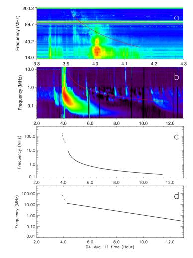
In order to illustrate an example of a m-to-DH type II radio burst event, we include (Figure 1a-d) the frequency-time drift graphs on 2011-August-04. Figure1a shows the trace of second harmonic component of the type II emission over-plotted on the dynamic spectrum observed by the Culgoora radio spectrograph in the m domain. To make the tracing of the type II emission in the frequency-time $(f-t)$ frame, we first pinpointed the second harmonic emission along a straight line in the $1/f-t$ frame. Then the traced points were linearly fitted to produce the smooth curve in the $(f-t)$ frame. Similarly, the smooth curve in Figure 1b is the traced second harmonic component over-plotted in the dynamic spectrum observed by Wind/WAVES in the DH domain. To prove that the traced type II emissions in Figure 1a and 1b are from the same event, we plot them in the same figure as shown in Figure 1c. The type II emissions in m and DH domains are indicated by dashed and solid lines, respectively. We can see in this figure that besides the time continuation, the slopes $(df/dt)$ of the two traced branches have a smooth transition from m to DH domains around 04:12 UT. Furthermore, the drift graph for m-to-DH type II burst based on Prakash et al. (2009) is shown in Figure 1d.
The start, peak, and end times (not listed in Wind/WAVES catalog) of the flares are taken from the GOES (Geosynchronous Operating Environmental Satellite) soft X-ray data³³3 $ftp://ftp.ngdc.noaa.gov/STP/space-weather/solar-data/solar-features/solar-flares/x-rays/goes/.$ by checking the source location of the CMEs and the corresponding flare class. The CME onset time ( onset time reported in the catalog is estimated by back-extrapolating the CME height time data to 1 R_∘ from the constant-speed approximation method), first appearance time (it represents the time of CME at its first appearance in the LASCO C2/C3 field of view), residual acceleration (obtained from a quadratic fit to the height time measurements within the LASCO FOV) of CMEs⁴⁴4 $http://cdaw.gsfc.nasa.gov/CME_{l}ist/index.html.$ are also obtained from the SOHO/LASCO (Solar and Heliospheric Observatory/Large Angle and Spectrometric Coronagraph) catalog, maintained by the NASA s CDAW data Center (Yashiro et al., 2004; Gopalswamy et al., 2009).

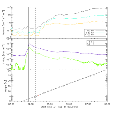
For each event, we plotted and visually examined the proton flux ( $>$ 10 MeV), and also conformed their spatial and temporal association from CDAW major SEP events list⁵⁵5 $https://cdaw.gsfc.nasa.gov/CME_{l}ist/sepe/.$ . Out of 48 events, 31 (24 major (Ip $\geq$ 10) and 7 minor SEP events (1pfu $\leq$ Ip $\leq$ 10 pfu)) m-to-DH type II radio bursts were found to associate with SEP events and the remaining 17 of them were not associated with SEP events. As an example, SEP proton flux, GOES X-ray light curves, and CME height-time diagram for one of the 31 selected events associated with SEPs, are shown in Figure 2. This SEP-associated CME (with an average sky-plane speed of 1315 km s^-1) responsible for the m-to-DH type II burst was a full halo CME ejected from source location N19W36 close to the disk center. It was first observed by the C2 coronagraph in LASCO at a height of 4.08 R_∘ at 04:12 UT. It was more decelerated due to the aerodynamic drag with a mean residual deceleration of –41.1 m s^-2 within the LASCO Field of view (FOV).The height where it achieved the sky-plane peak speed (2069 km s^-1) was nearly 5.96 R_∘. It is shown in red colored data point in the height-time plot (bottom panel of Figure 2). This CME was also associated with a gradual M class solar flare (M9.3) with a duration of 23 min. After nearly 18 min of first appearance of the CME, the particle enhancement was observed by the GOES in the energy channel $>$ 10 MeV at 04:30 UT and it reached the peak intensity of 90 pfu at 21: 50 UT on 2011-August-05.The m and DH type II bursts formed at 03:53 UT and 04:15 UT, respectively during the rising and decaying phases of the solar flare. The particle acceleration happened only after the DH type II emission from the outer corona. For convenience of descriptions, hereinafter, a CME, flare, m and DH type II radio burst associated with/without a SEP event are called as SEP-associated/non-SEP-associated events.
In Table 1, the basic properties of m-to-DH type II bursts are given. In this table, the date of the event (yymmdd) is given in Column 1. Columns 2 6 give the m type II properties: starting and ending times of the events in UT in Columns 2 and 3, starting and ending frequencies of m type II radio bursts (in MHz) in Columns 4 and 5, and the m type II shock speed (as listed in Culgoora online type II catalog) in column 6. Similarly, the properties of DH type II events are shown in Columns 7-10 (Columns 7 and 8 correspond to the starting and ending times of DH type II events in UT, and Columns 9 and 10 give the starting and ending frequencies of DH type II radio bursts in kHz). Column 11 defines whether type II bursts-associated-shocks and/or flares produced SEPs (Yes), or not (No). Please note that for few events, DH type II started slightly earlier than the end time of the m type II bursts. For an example, the 990604 event had m type II burst s ending time at 07:10 in 30 MHz, but DH type II emission started little earlier at 07:05 in 14 MHz. This is possibly due to the complexity of the type II emissions in these events where the precise determination of m type II end time (and/or a precise DH type II start time) is very difficult. The several-minute advance of the DH type II emission could therefore be interpreted as an uncertainty of the start/end time determination.
In Table 2, we compile the data on the soft X-ray flares and CMEs which are associated with m-to-DH type II bursts. First column gives the date of events; Columns 2 6 describe the X-ray flare events: Columns 2 4 give the start, end and peak times of the flare events in UT, respectively; Column 5 shows the locations of flares and flare peak flux is presented in Column 6. The X-ray flare is classified as A, B, C, M and X according to the peak flux intensity $<$ 10^-7, 10^-7 – 10^-6, 10^-6 – 10^-5, 10^-5 – 10^-4 and $\geq$ 10^-4 W m^-2, respectively. The numerical value after the class refers to the multiplicity factor. Columns 7 12 give the characteristics of the CMEs; Columns 7 and 8 are the onset and times of first appearance of CME in LASCO FOV in UT; central position angle and width are given in Columns 9 and 10. Columns 11 and 12 represent the CMEs mean sky-plane speed and residual acceleration, respectively.
The statistical values (mean and median) of the parameters describing properties of CME, soft X-ray flares, delay times and m and DH type II bursts separately for SEP and non-SEP events are presented in Table 3. In Column 1 the names of phenomena are given. Column 2 denotes the properties of the considered events. Columns 3-4 and 5-6 give the estimated mean and median of the considered parameters for SEP-associated and non-SEP-associated events, respectively. The type II formation heights listed in the table are obtained from the back extrapolation method, addressed in Section 3.5.1. In the next section we present statistical analyses of these two sets of events.

3 Results and discussion

3.1 Characteristics of SEP-associated and non-SEP-associated CMEs

Kinematics and width are important properties of CMEs for understanding their production of SEP events. An extensive investigation of various CME speeds (sky-plane speed, projection corrected speed, and peak speed of the sky-plane), acceleration, and width is presented in this section.
The sky-plane speeds are the average speeds of the CMEs within the LASCO FOV obtained by using the linear fit to the height time measurements. But sky-plane speed is only the projected speed of the CMEs. From the LASCO coronagraph images we can only detect apparent speeds and widths of CMEs. The three-dimensional structure and actual speeds of CMEs remain unknown due to the projection effect, especially for disk CMEs (source longitude $\leq$ 60^∘). Considering a set of energetic CMEs, Gopalswamy et al. (2000) demonstrated that the projection effect of speeds of the halo CMEs depends on the longitude (Pappa Kalaivani et al., 2010; Gopalswamy et al., 2007). The projection corrected speed (real propagation speed) and width of halo CMEs can be obtained, among several methods, from a cone model (Michałek et al., 2003; Xie et al., 2004), it is deduced from the sky-plane speed by using the approximation method. We adopted the arguments of Gopalswamy et al. (2009) to assign an average half width $(\omega)$ to each speed range and took it as the cone half angle: 66^∘ $(V_{sky}$ $>$ 900 km s ${}^{-1})$ , 45^∘ (500 km s^-1 $<$ $V_{sky}$ $\leq$ 900 km s^-1), and 32^∘ ( $V_{sky}$ $<$ 500 km s^-1). The CME corrected speeds were calculated by using the relation $V_{corrected}=(cos\omega+sin\omega)/(cos\omega cos\theta+sin\omega)\times V_{sky}$ where $\theta$ is the angle between the cone axis and sky-plane obtained from the heliographic coordinates of the source. From this equation, we estimated the corrected speeds of partial and full halo CMEs. The residual acceleration from the CDAW SOHO/LASCO CME Catalog was also derived from the height-time measurement. It is called as residual acceleration because the acceleration due to gravity and the propelling forces must have declined significantly, while the deceleration due to drag becomes dominant at heights corresponding to the LASCO FOV.

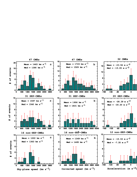
The distributions of sky-plane speed (a), corrected speed (b) and residual acceleration (c) of all events for which these properties could be determined (top) SEP-associated CMEs (middle) and non-SEP-associated CMEs (bottom) are shown in Figure 3. The difference between the mean sky-plane speed of SEP-associated CMEs and non-SEP-associated CME events (1587 km s^-1) and 1222 km s^-1), respectively) is statistically significant (student t-test shows there is P = 5% chance that the difference is accidental). Prakash et al. (2010) also found that a set of CMEs associated with the m-to-DH type II radio bursts have the mean sky-plane speeds equal to 1655 km s^-1. However, the mean sky-plane speed of all CMEs (1463 km s^-1) is nearly three times greater than average CMEs (Gopalswamy et al., 2001; Prakash et al., 2012). The error bars plotted in each bin for all figures are given by the calculation with 84.13% of confidence level for upper and lower limits for small number of counts. They are based on standard equations derived from the Poisson and binomial statistics (Gehrels, 1986).
The distribution of the projection corrected speed is shown in Figure3b. The student t-test shows that the difference between the mean corrected speeds of SEP-associated CMEs and non-SEP-associated CME events (1906 and 1369 km s^-1)) is statistically significant (P =2 %). Recently, Gopalswamy et al. (2012) studied the properties of a set of 16 GLE (Ground Level Enhancement) events. They found that, the mean (median) projection corrected speed of this set of events was 2083 km s^-1 (1937 km s^-1), which is slightly larger than that of our mean value.
The distributions of residual acceleration of all CMEs (top), SEP-associated CMEs (middle) and non-SEP-associated CMEs (bottom) are shown in Figure 3c. The residual acceleration of all CMEs varies from –160 m s^-2 to 35 m s^-2 (mean = –23.56 m s^-2). The number of events in residual acceleration panels is reduced due to the restriction of sample of events. To get reliable values of acceleration we limited our study to events having at least four height-time data points, i.e. those events without asterisk in Column 12 of Table 2 (Gopalswamy et al., 2001; Yashiro et al., 2004). The mean difference between residual acceleration of SEP-associated CMEs and non-SEP-associated CME events (–28.39 m s^-2 and –15.53 m s^-2, respectively) is statistically insignificant (P=41%). However, if we exclude the two outliers (a highly decelerated event from each group) of SEP-associated CMEs and non-SEP-associated CMEs, the mean values are reduced to –21.52 m s^-2 and –5.63 m s^-2, respectively and it is statistically quite significant (P=8%). From this result, we infer that SEP-associated CMEs are three times more decelerated than the non-SEP-associated CMEs. This result is consistent with Vršnak et al. (2004) and Belov et al. (2014) that CMEs having high initial speed are mostly decelerated. From the present study, the mean sky-plane, corrected speeds of SEP-associated CMEs are much larger than non-SEP-associated CMEs. Due to the high initial speeds of SEP-associated CME events, they are more decelerated than the non-SEP-associated CMEs.
To determine the sky-plane peak speed and its corresponding height, initially we selected height-time data from the CDAW CME list and then smoothed these data. In order to find the sky-plane peak speed, we took the time derivative between each two height-time data points. From these values, we picked out the maximum (peak) speed and their corresponding height for our further analysis. The distribution of the sky-plane peak speed heights (a) and peak speed (b) for set of all CMEs (top), SEP-associated CMEs (middle) and non-SEP-associated CMEs (bottom) are shown in Figure 4. The 10% of uncertainties in the estimation of sky-plane peak speed and their height is unavoidable. This may be due to the projection effect of disk events and also the different time cadences of LASCO C2 and C3 coronagraphs (Prakash et al., 2012).

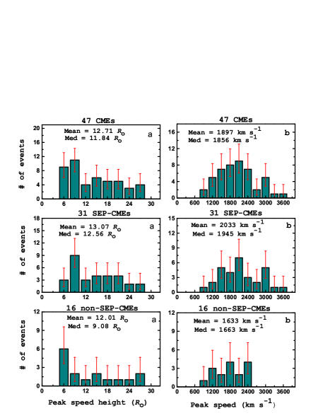
In this study, nearly half of m-to-DH type II radio bursts (all events) associated CMEs achieved their sky-plane peak speed within 12 R_∘ (median = 11.84 R_∘). The mean sky-plane peak speeds and their heights are distributed symmetrically. The t-test shows that difference between the average peak speed heights of SEP-associated CMEs and non-SEP-associated CME events (13.07 and 12.01 R_∘, respectively) is statistically insignificant. In both cases, CMEs reached their sky-plane peak speeds at nearly the same height. From this result, we reveal that the initial accelerating phase of all CMEs was continued in average up to 12 R_∘ (as seen from the Figure 4a-top). Recently, Gopalswamy et al. (2012) and Prakash et al. (2012) also estimated the sky-plane peak speed height of a set of CMEs. They found that decelerating CMEs achieved their sky-plane peak speed at lower heights than the accelerating CMEs. Our result slightly differs from the other previous studies. In our case, more decelerated SEP-associated CMEs attained their peak speeds at larger heights (13.07 R_∘) than non-SEP-associated CMEs (12.01 R_∘).
The distribution of the sky-plane peak speeds of CMEs associated with all CMEs (top), SEP-associated CMEs (middle) and non-SEP-associated CMEs (bottom) are shown in Figure 4b. The average peak speed of CMEs associated with all events (m-to-DH type II radio bursts) is 1897 km s^-1 (median = 1856 km s^-1). Interestingly within the average peak speeds height, the SEP-associated CMEs achieved higher speed (median=1945 km s-1) than that of non-SEP-associated CMEs (1663 km s^-1)). The difference between the mean sky-plane peak speed of SEP-associated CMEs and non-SEP-associated CMEs (2033 km s^-1 and 1633 km s^-1), respectively) is statistically significant (P=3%).
The CME width seems to be a critical parameter to determining the kinetic energy of the CMEs (Gopalswamy et al., 2001). The DH type II bursts were also closely linked to CMEs which are faster and wider than average CMEs (Gopalswamy et al., 2001). The CME widths are one of the important parameter to decide SEP intensity (Kahler et al., 1984). Therefore, we studied the widths of the two populations of CMEs. However, it is difficult to assess the true width of halo CMEs. Note that the true width of halo CMEs cannot be determined from the 2D images because of the projection effect, especially for the disk event (longitude within $\pm$ 60^∘). In our case, most of the CMEs originated from the disk center. Furthermore, the most of the SEP-associated CMEs (81%) are full halo and only 56% of non-SEP-associated CMEs are full halo. It should be noted that the mean apparent widths of the SEP-associated CMEs are slightly larger than the non-SEP-associated CMEs (330^∘ and 274^∘, respectively; please note that these distributions are not shown). Recently, (Prakash et al., 2014) reported the widths of CMEs for a set of m-to-DH type II bursts associated geoeffetive CMEs. They found that the widths of the geoeffective CMEs (339^∘) is considerably larger than non geoeffective CMEs (251^∘).

3.2 The CME speeds – SEP peak intensity relationship

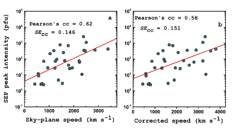
The relationship between the sky-plane speed and corrected speeds of CMEs with peak intensity of the associated SEP events is shown in Figure 5. The speed of the CMEs should correlate reasonably well with the peak intensity of the associated SEP events (Kahler et al., 1984; Reames, 1999; Kahler, 2001; Gopalswamy et al., 2003) as one would expect when the particles are accelerated by the CME-driven shocks. Here, we also assume that protons are accelerated due to CME-driven shocks. In Figure 5, we found positive correlation between CME speeds (sky-plane speed and corrected speed) and the logarithmic peak intensity of SEP events. The estimated Pearson s correlation coefficients are cc = 0.62 and cc = 0.58, respectively. Although the SEP peak intensity is generally correlated with the CME speed, the scatter is very large. We also calculated the standard error of the correlation coefficient (SE_cc) by using $SE_{cc}=\sqrt{(1-cc^{2})/(n-2)}$ , where n is the number of data points. The linear fitting functions of speed and intensity are indicated by the red straight lines. Recently, Papaioannou et al. (2016) found that there is a good correlation between CME speed and proton peak flux (cc = 0.57) for a different set of events and their standard error is around 0.07 (sample events are much larger than that of ours). From these studies, we infer that the speed of the CME associated with m-to-DH type II bursts may influence the peak intensity of the SEP events. Hence, these SEP-associated CMEs are very likely good electron and proton accelerators. Our results are consistent with previous studies (e.g., (Gopalswamy et al., 2005; Ding et al., 2013; Subramanian & Shanmugaraju, 2016; Papaioannou et al., 2016).

3.3 Characteristics of SEP-associated and non-SEP-associated flares

The flare rise time (time interval between flare start and flare peak) is the most important parameter in analyzing the relationship between flares, CMEs and type II radio bursts (Shanmugaraju et al., 2003; Subramanian et al., 2003; Zhang et al., 2004; Prakash et al., 2009, 2012). The distribution of rise times (a), duration (b), and peak flux (c) of all 45 events (top) SEP-associated flares (middle) and non-SEP-associated flare (bottom) events is shown in Figure 6. As seen from this figure, the average flare rise time of the 45 events with reported flares (see Table 2) is nearly equal to 28.51 min (median = 21 min). Most of the flares (71%) reach the peak time within 30 min. There is no difference between the mean rise time of SEP-associated flares and that of non-SEP-associated flares (28.90 and 27.64 min, respectively). The t-test shows that the mean difference is statistically insignificant. Recently, Prakash et al. (2012) found that for eruptions associated with DH type II bursts, the median rise time of the flares associated with accelerating CMEs is larger than that in association with decelerating CMEs (median = 40.5 and 21.0 min).

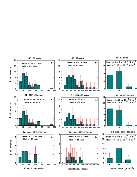
The distribution of duration for 45 events (top), SEP-associated flares (middle) and non-SEP-associated flares (bottom) are shown in Figure 6b. For all m-to-DH type II radio bursts, associated flare duration (the interval from the start to end) varies from 10 160 min. The mean durations of both sets of events are nearly equal (50 min). Recently, Prakash et al. (2010) found that the average duration of the flares associated with m-to-DH type II bursts was 54.24 min. Interestingly, the duration of SEP-associated flares is much lower than the flares associated with geoeffective events (74 min) events (Prakash et al., 2014). The propelling Lorentz force acts longer for geoeffective CMEs (it is consistent with the longer flare duration (or rise time)). But for SEP-associated CMEs the Lorentz force should be acting for a shorter time, so the Lorentz force and gravity decrease, the drag force becomes the dominant force because of the widths of the CMEs, and so they tend to decelerate more in the LASCO FOV (Vršnak et al., 2004).
In Figure 6c, the distributions of peak flux of the 45 events with reported flares (top), SEP-associated flares (middle) and non-SEP-associated flares (bottom) are plotted. It should be noted that 48% of SEP-associated flare and 21% non-SEP-associated flare belongs to X class events, respectively. The differences in mean peak flux of SEP-associated flares and non-SEP-associated flares, 1.85 $\times$ 10^-4 W m^-2 and 5.98 $\times$ 10^-5 W m^-2, respectively is statistically significant (P = 5%). The X-ray peak flux of SEP-associated flares (1.85 $\times$ 10^-4 W m^-2) is stronger than that of geoeffective storm associated flares (0.77 $\times$ 10^-4 W m^-2).

3.4 Time delays between the properties of flares, CMEs and type IIs for SEP-associated and non-SEP-associated events

We examined the time delays (relative timings) between properties of m-to-DH type II bursts, flares and CMEs for SEP-associated and non-SEP-associated events (see Table 3, note that these distributions are not shown). We have considered the delay times between the onset of CMEs (back-extrapolated time) and starting time of m and DH type II radio bursts. The mean time delays between the onset times of CMEs and starting time of m type II bursts for SEP-associated events is lower than that of non-SEP-associated events (10 and 16 min, respectively) and it is statistically insignificant. However, the difference of the average time delays between the onset times of CME and starting time of DH type II bursts for SEP-associated and non-SEP-associated events are 26 min and 34 min, respectively. It has quite low statistical significance (P = 10%).
Similarly, the time delays between flare onset and starting time of m type II burst ranges from 5 to 67 min. The 94% of m type II associated with SEP events originated within the rising phase of the flare. But 78% of non-SEP-associated events are formed before the peak of flare. However, there is no significant difference between the mean time delays between the flare onset and m type II bursts start for SEP-associated and non-SEP-associated events (19 min for both). On the contrary, the mean delay time between the flare onset and starting time of DH type II bursts for SEP events is lower than the time delays of non-SEP-associated events (34 and 40 min, respectively). The 52% and 28% of the SEP-associated and non-SEP-associated DH type II emission originated during rising phase of the flares. The average delay time between the beginning of the m and DH type II burst of SEP-associated events is slightly lower than that of non-SEP-associated events (16 and 21 min, respectively). From these results, we infer that the longer flare type II delay may be related to the possibility that the shock forms at larger distance where the CME becomes super-Alfv nic (Gopalswamy et al., 2001).

3.5 Characteristics of m and DH type II for SEP-associated and non-SEP-associated events

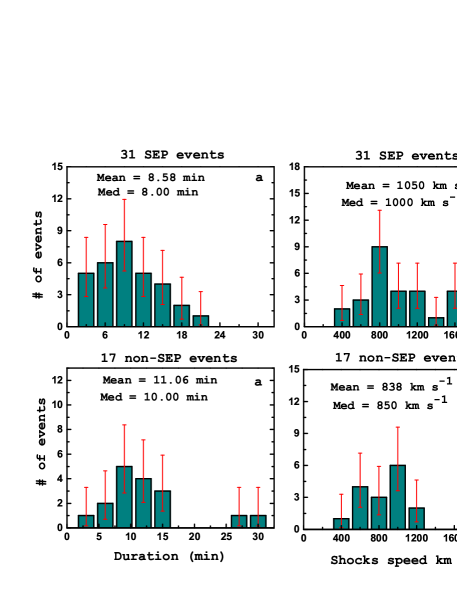
In this section, we have performed similar analysis to study the characteristics of m and DH type II bursts for both sets of events. The drift rate is determined from starting and ending frequencies, and the duration (T_d) of m and DH type II bursts $[df/dt=(fs-fe)/Td]$ , where subscripts s and e stand for the starting and ending fre-quencies of type II radio emission. The distributions of the duration (a) and shock speed (b) of m type II bursts for SEP-associated (top) and non-SEP-associated (bot-tom) events are presented in Figure 7. As seen from this figure, the duration of the m type II bursts for both sets of events ranges from 3 to 29 min. There is no significant difference between the median duration of m type II bursts for SEP-associated and non-SEP-associated events (8 and 10 min, respectively). Most of the m type II bursts have the duration around 10 min. Our result is consistent with previous results (Shanmugaraju et al., 2003; Prakash et al., 2010; Vasanth et al., 2011; Prakash et al., 2014).
The differences between the mean starting frequencies of m type II bursts for SEP-associated and non-SEP-associated events is statistically insignificant (86 and 76 MHz, respectively; please note that these distributions are not shown). However, 68% of SEP-associated m type II bursts have the starting frequencies below 100 MHz, and the remaining 32% of events have relatively higher starting frequency ( $>$ 100 MHz). This result is different from that for a set of geoeffective CMEs associated with m type II bursts studied by Prakash et al. (2014).

They found that 62% of m type II bursts associated with geoeffective CMEs have starting frequencies above 100 MHz, and the remaining 38% of events have starting frequencies below 100 MHz. We also examined the difference between the ending frequencies of m type II bursts associated with both sets of events. There is no significant difference between the ending frequencies of m type II bursts for SEP-associated and non-SEP-associated events (25 and 23 MHz, respectively). However, the drift rate of m type II radio bursts associated with SEPs events is higher than for the non-SEP associated m type IIs. The difference between the mean drift rates of m type II radio bursts for SEP-associated and non-SEP-associated events (0.17 and 0.10 MHz s^-1) is statistically significant (P= 5%). From this result, we infer that SEP-associated m type II shocks travelled with higher speeds than non-SEP-associated shocks.
The distribution of shock speed derived from m type II radio bursts for SEP-associated (top) and non-SEP-associated (bottom) events is shown in Figure 7b. As seen from this figure, SEP-associated m type II shocks have higher speed (1050 km s^-1) than that of non-SEP-associated events (838 km s^-1). It is consistent with our previous result, the drift rate of the m type II bursts for SEP-associated (0.17 MHz s^-1) events are larger than non-SEP-associated events (0.10 MHz s^-1). The difference between the average shock speed of m type II burst for SEP-associated and non-SEP-associated events is quite statistically significant (P = 8%).
Figure 8 shows distributions of the duration (a) and ending frequency (b) of DH type II radio bursts for SEP-associated (top) and non-SEP-associated events (bottom). The durations of all DH type II bursts range from 17 min to 2650 min. However, most DH type II bursts have durations within 500 min. The peak of the distribution lies at 200 min for both sets of events. The difference between the mean durations (531 and 304 min, respectively) of the DH type II radio bursts for SEP-associated and non-SEP-associated events is statistically insignificant (P = 22%).

The starting frequencies of both sets of events do not differ much because most of DH type II bursts have starting frequencies around the upper cut-off frequency of the WAVES instrument (14 MHz). The distribution of ending frequencies of DH type II bursts for SEP-associated (top) and non-SEP-associated (bottom) events is shown in Figure 8b. It is noted that 58% of SEP-associated DH type II bursts enter into the km domain ( $<$ 300 kHz). On the other hand, only 29% (5/17) of non-SEP-associated events reach the km domain. The differences between the mean ending frequencies of DH type II bursts for SEP-associated and non-SEP-associated events (522 and 1476 kHz, respectively) are quite statistically significant (P = 6 %). The ending frequency of type II bursts reflects the kinetic energy of CME (Gopalswamy et al., 2005). It implies that the SEP-associated CMEs have larger kinetic energy than the non-SEP-associated CMEs.
We also examined the drift rate of DH type II bursts for SEP-associated and non-SEP-associated events. We found that the average drift rate for SEP-associated DH type II bursts is lower than non-SEP-associated events (1.08 and 1.92 kHz s^-1, respectively). The t-test shows that the difference between the mean drift rate of these two populations is also statistically quite significant (P = 8 %). It should be noted that, in comparison with non-SEP-associated type II bursts, SEP-associated type II bursts have higher drift rate in the m domain and lower drift rate in DH domain. This difference is in agreement with the fact that SEP-associated CMEs decelerate more than non-SEP-associated CMEs.

3.6 Type II Formation height

Based on delay time studies, the type II formation height is much closer to Sun for SEP-associated events and larger distance for non-SEP-associated events. In this section, we examined quantitatively the type II formation in coronal and interplanetary medium statistically. It is believed that type II radio bursts are generated by the shock formed around a CME moving at a speed faster than the local magnetosonic speed. It is still under debate where exactly the type II source locates at the shock front. For the metric type II source, some authors claimed that it is due to the shocks formed as a result of the expansion of the CME flanks (Cho et al., 2008; Liu et al., 2009), while some other authors believed that the shock ahead of the CME nose is a preferable place (Ramesh et al., 2012). For the DH type II source, different opinions also exist. For instance, Magdalenić et al. (2014) found that the type II sources were close to the flank for the CME they investigated. However, Martínez Oliveros et al. (2012) found that the shock ahead of the CME nose is more favorable for producing type II emission (Shen et al., 2013). In this section, the type II formation height was derived from two different methods. A straight-forward method is the inversion of the density corresponding to the starting frequency to a height using some analytical density model. However, the inverted heights may subject to large error bars due to the large uncertainties of density models. Therefore we also computed the type II formation height from the back extrapolation of the CME height to the height at the type II start time under the assumption of a constant CME speed. The values listed in Table 3 are from the back extrapolation method.
A straight-forward method to estimate the type II formation height is to use the relationship between the plasma frequency fp and electron density ne given by $f_{p}=9\times 10^{-3}\sqrt{n_{e}}$ MHz the type II bursts observed at local plasma starting (f_s) and ending frequencies (f_e) were used to get information about the plasma density (n_e) during the starting and ending frequencies of type II emission. From these densities, one can estimate the two different heights (formation and ending height) of coronal shocks by using the one-fold Newkirk $n_{e}=4.2\times 10^{4}\times 10^{4.32(R_{\circ}/R)}$ electron density model (Newkirk, 1961). We estimated the m type II formation height by using the starting frequencies; it varies in the ranges 1.45 1.86 R_∘. We also found the ending heights of m type II emission ranges from 1.73 to 3.15 R_∘. The difference in the mean value of formation height of m type II emission for SEP-associated and a non-SEP-associated event (1.41 and 1.64 R_∘, respectively) is statically insignificant.
As the density model is subject to large uncertainties, we also checked type II formation height using the back extrapolation of the CME height at the type II start time under an assumption of a constant CME speed. As in Gopalswamy et al. (2009), another assumption we made is that the heliocentric distance of the m type II burst (and of the shock) can be approximated by that of the driving CME, more specifically, the leading edge distance. Consequently, the height can be simply derived from the observation of SOHO/LASCO using this relation $H_{typeII}=R_{c}-V_{c}\times T_{cv}$ , where R_c is the first appearance position of CMEs in LASCO C2/C3 field of view, T_cv is the time delays between the first appearance time of the CME and the start time of the m and DH type II burst. We assigned two different CME speeds (V_c) to determine the formation height of m and DH type II radio bursts respectively. For a m type II burst, Vc is the initial speed estimated from the first two height-time data points within the LASCO FOV. For a DH type II burst, we utilized the projection corrected speed calculated from the sky-plane speed (as described in Section 3.1) within the full LASCO FOV. The constant speed method (linear speed assumption) has been used by several authors (Harrison, 1986, 1995; Moon et al., 2002; Zhang et al., 2002; Andrews, 2003; Cho et al., 2003) to estimate the CME onset times, since we have insufficient kinematic information of CMEs at the time of type II radio bursts in many cases. The impulsive acceleration phases of the CMEs are coincident with the impulsive phases of GOES X-ray flares, and their accelerations nearly stop after the flare peak times (Zhang et al., 2001; Neupert et al., 2001; Shanmugaraju et al., 2003). In our case, most of the type IIs started just before the flare peak times or after. So the speeds of flare-associated CMEs are nearly constant at the coronal region from 1.4 to 2.4 R_∘ (MacQueen & Fisher, 1983).

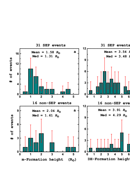
These facts imply that the errors of the linear extrapolated heights at the time of type II radio bursts are less serious than in the case of CME onset time estimates. The formation height of m (a) and DH type II bursts (b) for SEP-associated (top) and non-SEP-associated (bottom) events are shown in Figure 9. As seen from this figure, 71% and 43% (SEP and non-SEP-associated events, respectively) of the formation height of m type II bursts lies within 1.5 Ro. The median formation heights of m type II bursts for SEP-associated and non-SEP-associated events (1.31 and 1.61 Ro, respectively) are nearly equal. The student t-test also shows that the difference between the mean values of these two populations (1.58 Ro and 2.04 R_∘) is statistically insignificant (P = 26%). The median formation heights are well consistent with the estimated formation height using the Newkirk model previously. Mäkelä et al. (2015) analyzed the heights of a different population of CMEs at the onset of m type II bursts using the flare onset method. They obtained the mean m type II formation height is 1.72 R_∘ (median= 1.6 R_∘). Their results are slightly higher than the values in this paper. This could be partially due to the projection effect and/or the different methods of the formation height calculation.
We also estimated the formation height of DH type II bursts for SEP-associated (top) and non-SEP-associated (bottom) events shown in Figure 9b. In this study, nearly 61% and 75% of DH type II bursts for SEP and non-SEP-associated events are formed after 2.5 R_∘. The t-test shows that difference between the mean DH type II formation height for SEP and non-SEP-associated events (3.54 and 3.91 R_∘) is statistically insignificant (P = 51%). One possible interpretation of the insignificance is that quite a few events, either SEP or non-SEP, have a starting frequency close to the ionospheric cutoff frequency of radio emissions. Therefore, we do not see much difference of the formation height between SEP and non-SEP events.

3.7 Source locations

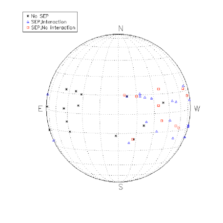
The distribution of the source location of 44 m-to-DH type II bursts events for SEP-associated and non-SEP-associated events are shown in Figure 10. From this figure, it should be noted that for all events, 73% (32/44) originated from the disk center (longitude within 60o). We also see that, 93% of SEP-associated events are from the western side of the solar disk. On the other hand, 77%of non-SEP-associated events originated from the eastern side. Furthermore, 67% of the SEP-associated events sources lies within the disk center and the remaining 33% of events from the limb, events are those with longitudes larger than 60^∘. Out of 31 SEP-associated events, 20 (65%) events are associated with CME-CME interaction and remaining 11 (35%) events are non-interacting CMEs. The CME-CME interaction was examined by checking the position angle (PA) and time coincidence of primary SEP-associated CMEs and preceding one or more slow CMEs. It was also confirmed from the LASCO movies. The CMEs interaction is an important factor to decide whether CMEs are associated with SEP events or not (Shanmugaraju & Prasanna Subramanian, 2014). We also infer that the m-to-DH type II bursts associated solar flares and CMEs from the western hemisphere have a high possibility to be associated with SEPs that can be detected at Earth, also directly related with the connectivity of the magnetic spiral with Earth, is consistent with previous studies (Wang et al., 2002; Gopalswamy et al., 2002; Zhang et al., 2004, 2007; Prakash et al., 2014; Vasanth et al., 2015).
We noticed that two events with their longitudes west of W15 did not produce SEPs as expected. For these two events, the shock speeds are lower than the average shock speed in the group of SEP- associated events. Probably the shock strength is not large enough to accelerate the $>$ 10 MeV protons to above 10 pfu which is our definition of a SEP event. Nevertheless, we checked the flux of some lower energy particles and they did show some enhancement related to these two events. On the other hand, we found that two events very close to the eastern limb were unexpectedly associated with SEPs. As these two events are interacting events, the propagation directions might be deflected after the primary CMEs erupted from their source regions. As a shock usually has a large extent in longitude, the accelerated SEPs may arrive the Earth.

4 Summary and Conclusion

We have identified a set of m-to-DH type II bursts, solar flare and CMEs based on the Prakash et al. (2009), recorded during period of April 1997 October 2012 (SC 23 and SC 24). Out of 48 m-to-DH type II bursts associated with flares and CMEs, 31 (65%) of them identified as SEP-associated events and the remaining 17 events could be interpreted as non-SEP-associated events. We analyzed the characteristics of m-to-DH type II bursts, CMEs, solar flares associated with SEP and non-SEP events. The main results of our study can be summarized as follows. The mean sky-plane speed of SEP-associated CMEs is nearly three times as large as the mean sky-plane speed of average CMEs. There is a significant difference in the mean sky-plane speed of SEP-associated CMEs and non-SEP-associated CME events (1587 km s^-1 and 1222 km s^-1, respectively). The average projection corrected speed (real propagation speed) of SEP-associated CMEs is larger than that of the non-SEP-associated events (1906 and 1369 km s^-1). The SEP-associated CMEs found to be more decelerated than the non-SEP-associated CMEs within the LASCO FOV (–21.52 m s^-2 and –5.63 m s^-2, respectively). This implies that the mean residual acceleration of SEP-associated CME events is three times as great as the mean residual acceleration of the non-SEP-associated CMEs. The average apparent width of the SEP-associated CMEs is larger than the non-SEP-associated CMEs (330^∘ and 274^∘).
The SEP-associated CMEs and non-SEP-associated CMEs achieved their sky-plane peak speed at nearly same heights (13.07 and 12.01 R_∘, respectively), but sky-plane peak speed of the SEP-associated CMEs (2033 km s^-1) is much larger than that of non-SEP-associated CMEs (1633 km s^-1). These results reflect that SEP-associated flares are stronger than the non-SEP-associated flares (1.85 $\times$ 10^-4 and 5.98 $\times$ 10^-5 W m^-2) even though the flare rise time (28.90 and 27.64 min) and duration (50 min) of both sets of events are nearly equal. As described earlier, the stronger flare implies that we have prolonged action of the Lorentz force (Vršnak, 2008). We found positive Pearson s correlation between the speeds of CMEs (sky-plane speed and corrected speed) and logarithmic peak intensity of SEP events (cc = 0.62 and cc = 0.58, respectively). The delay time between m and DH type II bursts for SEP-associated events is smaller in average than non-SEP-associated events (16 and 21 min, respectively).
There is no much difference between the duration, starting and ending frequencies of m type II bursts for SEP-associated and non-SEP-associated events. But the shock speed (1050 km s^-1 and 838 km s^-1) and drift rate (0.17 and 0.10 MHz s^-1) of m type II bursts for SEP-associated events are larger than the non-SEP-associated events. In case of DH type II burst, there is no difference between the starting frequencies of both sets of events. But the differences in the mean duration between SEP-associated and non-SEP-associated events (531 min and 157 min, respectively) is statistically high significant (P = 0.001%). The 58% of SEP-associated DH type II radio bursts enter into the km domain ( $<$ 300 kHz, m-to-km type II bursts). On the other hand, only 28% of non-SEP-associated DH type II events enter into the km domain. The mean difference between the ending frequencies (522 and 1476 kHz) and drift rates (1.08 and 1.92 kHz s^-1) of DH type II bursts for SEP-associated and a non-SEP-associated event is quite statistically significant. The average shock formation height of m (1.58 R_∘ and 2.04 R_∘) and DH type II bursts (3.54 R_∘ and 3.91 R_∘) for SEP-associated and non-SEP-associated event slightly differs. We found that 93% of SEP-associated events from the westerns side of the solar disk and interestingly 65% of SEP events are due the interaction of CMEs. From this study, at least for the set of CMEs associated with m-to-DH type II bursts, SEP-associated CME events are more energetic than those not associated with SEPs, thus indicating that they are effective particle accelerators.

Acknowledgements We thank the referee for useful constructive comments to improve the quality of this manuscript. We greatly acknowledge the data support provided by various online data centers of NOAA and NASA. We would like to thank the Wind/WAVES and Culgoora spectrograph teams for providing the type II catalogs. The SOHO/LASCO CME catalog is generated and maintained at the CDAW Data Center by NASA and The Catholic University of America in cooperation with the Naval Research Laboratory. SOHO is a project of international cooperation between ESA and NASA. This work is fully supported by NNSFC via grants 11233008, 11427803, 11473070, 11522328, and by MSTC via 2011CB811402. O. Prakash thanks to the Chinese Academy of Sciences for providing General Financial Grant from the China Postdoctoral Science Foundation. L. Feng also acknowledges the Youth Innovation Promotion Association and the research fund from the State Key Laboratory of Space Weather for financial support. G. Michalek was supported by NCN through the grant UMO-2013/09/B/ST9/00034.

References

Acuña et al. (1995) Acuña, M. H., Ogilvie, K. W., Baker, D. N., et al. 1995, Space Sci. Rev., 71, 5.
Anastasiadis (2002) Anastasiadis, A. 2002, Journal of Atmospheric and Solar-Terrestrial Physics, 64, 481
Andrews (2003) Andrews, M. D. 2003, Sol. Phys., 218, 261
Belov et al. (2005) Belov, A., Garcia, H., Kurt, V., Mavromichalaki, H., & Gerontidou, M. 2005, Sol. Phys., 229, 135
Belov et al. (2014) Belov, A., Abunin, A., Abunina, M., et al. 2014, Sol. Phys., 289, 3949
Bougeret et al. (1995) Bougeret, J.-L., Kaiser, M. L., Kellogg, P. J., et al. 1995, Space Sci. Rev., 71, 231
Cane & Lario (2006) Cane, H. V., & Lario, D. 2006, Space Sci. Rev., 123, 45
Cane et al. (2010) Cane, H. V., Richardson, I. G., & von Rosenvinge, T. T. 2010, Journal of Geophysical Research (Space Physics), 115, A08101
Cho et al. (2003) Cho, K.-S., Kim, K.-S., Moon, Y.-J., & Dryer, M. 2003, Sol. Phys., 212, 151
Cho et al. (2008) Cho, K.-S., Bong, S.-C., Kim, Y.-H., et al. 2008, Astron. Astrophys., 491, 873
Dierckxsens et al. (2015) Dierckxsens, M., Tziotziou, K., Dalla, S., et al. 2015, Sol. Phys., 290, 841
Ding et al. (2013) Ding, L., Jiang, Y., Zhao, L., & Li, G. 2013, Astrophys. J., 763, 30
Gehrels (1986) Gehrels, N. 1986, Astrophys. J., 303, 336
Gopalswamy et al. (2000) Gopalswamy, N., Kaiser, M. L., Thompson, B. J., et al. 2000, Geophys. Res. Lett., 27, 1427
Gopalswamy et al. (2001) Gopalswamy, N., Lara, A., Kaiser, M. L., & Bougeret, J.-L. 2001, J. Geophys. Res., 106, 25261
Gopalswamy et al. (2001) Gopalswamy, N., Yashiro, S., Kaiser, M. L., Howard, R. A., & Bougeret, J.-L. 2001, J. Geophys. Res., 106, 29219
Gopalswamy et al. (2002) Gopalswamy, N., Yashiro, S., Michałek, G., et al. 2002, Astrophys. J. Lett., 572, L103
Gopalswamy et al. (2003) Gopalswamy, N., Yashiro, S., Lara, A., et al. 2003, Geophys. Res. Lett., 30, 8015
Gopalswamy et al. (2005) Gopalswamy, N., Aguilar-Rodriguez, E., Yashiro, S., et al. 2005, Journal of Geophysical Research (Space Physics), 110, A12S07
Gopalswamy et al. (2007) Gopalswamy, N., Yashiro, S., & Akiyama, S. 2007, Journal of Geophysical Research (Space Physics), 112, A06112
Gopalswamy et al. (2009) Gopalswamy, N., Yashiro, S., Michalek, G., et al. 2009, Earth Moon and Planets, 104, 295
Gopalswamy et al. (2009) Gopalswamy, N., Thompson, W. T., Davila, J. M., et al. 2009, Sol. Phys., 259, 227
Gopalswamy et al. (2010) Gopalswamy, N., Xie, H., Mäkelä, P., et al. 2010, Astrophys. J., 710, 1111
Gopalswamy et al. (2012) Gopalswamy, N., MäKelä, P., Akiyama, S., et al. 2012, Journal of Geophysical Research (Space Physics), 117, A08106
Gopalswamy et al. (2012) Gopalswamy, N., Xie, H., Yashiro, S., et al. 2012, Space Sci. Rev., 171, 23
Gopalswamy et al. (2014) Gopalswamy, N., Xie, H., Akiyama, S., Mäkelä, P. A., & Yashiro, S. 2014, Earth, Planets, and Space, 66, 104
Gopalswamy et al. (2015) Gopalswamy, N., Xie, H., Akiyama, S., et al. 2015, Astrophys. J. Lett., 804, L23
Harrison (1986) Harrison, R. A. 1986, Astron. Astrophys., 162, 283
Harrison (1995) Harrison, R. A. 1995, Astron. Astrophys., 304, 585
Kahler et al. (1984) Kahler, S. W., Sheeley, N. R., Jr., Howard, R. A., et al. 1984, J. Geophys. Res., 89, 9683
Kahler (2001) Kahler, S. W. 2001, J. Geophys. Res., 106, 20947
Kahler & Vourlidas (2014) Kahler, S. W., & Vourlidas, A. 2014, Astrophys. J., 784, 47
Kallenrode (2003) Kallenrode, M.-B. 2003, Journal of Physics G Nuclear Physics, 29, 965
Klein & Posner (2005) Klein, K.-L., & Posner, A. 2005, Astron. Astrophys., 438, 1029
Kocharov & Torsti (2002) Kocharov, L., & Torsti, J. 2002, Sol. Phys., 207, 149
Lara et al. (2003) Lara, A., Gopalswamy, N., Nunes, S., Muñoz, G., & Yashiro, S. 2003, Geophys. Res. Lett., 30, 8016
Liu et al. (2009) Liu, Y., Luhmann, J. G., Bale, S. D., & Lin, R. P. 2009, Astrophys. J. Lett., 691, L151
Lugaz & Farrugia (2014) Lugaz, N., & Farrugia, C. J. 2014, Geophys. Res. Lett., 41, 769
MacQueen & Fisher (1983) MacQueen, R. M., & Fisher, R. R. 1983, Sol. Phys., 89, 89
Magdalenić et al. (2014) Magdalenić, J., Marqué, C., Krupar, V., et al. 2014, Astrophys. J., 791, 115
Mäkelä et al. (2015) Mäkelä, P., Gopalswamy, N., Akiyama, S., Xie, H., & Yashiro, S. 2015, Astrophys. J., 806, 13
Martínez Oliveros et al. (2012) Martínez Oliveros, J. C., Raftery, C. L., Bain, H. M., et al. 2012, Astrophys. J., 748, 66
Michałek et al. (2003) Michałek, G., Gopalswamy, N., & Yashiro, S. 2003, Astrophys. J., 584, 472
Moon et al. (2002) Moon, Y.-J., Choe, G. S., Wang, H., et al. 2002, Astrophys. J., 581, 694
Neupert et al. (2001) Neupert, W. M., Thompson, B. J., Gurman, J. B., & Plunkett, S. P. 2001, J. Geophys. Res., 106, 25215
Newkirk (1961) Newkirk, G., Jr. 1961, Astrophys. J., 133, 983
Pappa Kalaivani et al. (2010) Pappa Kalaivani, P., Umapathy, S., Shanmugaraju, A., & Prakash, O. 2010, Astrophys. Space Sci., 330, 237
Papaioannou et al. (2016) Papaioannou, A., Sandberg, I., Anastasiadis, A., et al. 2016, Journal of Space Weather and Space Climate, 6, A42
Payne-Scott et al. (1947) Payne-Scott, R., Yabsley, D. E., & Bolton, J. G. 1947, Nature, 160, 256
Prakash et al. (2009) Prakash, O., Umapathy, S., Shanmugaraju, A., & Vršnak, B. 2009, Sol. Phys., 258, 105
Prakash et al. (2010) Prakash, O., Umapathy, S., Shanmugaraju, A., Pappa Kalaivani, P., & Vršnak, B. 2010, Sol. Phys., 266, 135
Prakash et al. (2012) Prakash, O., Umapathy, S., Shanmugaraju, A., Pappa Kalaivani, P., & Vršnak, B. 2012, Astrophys. Space Sci., 337, 47
Prakash et al. (2012) Prakash, O., Umapathy, S., Shanmugaraju, A., & Vasanth, V. 2012, Sol. Phys., 281, 765
Prakash et al. (2012) Prakash, O., Umapathy, S., & Shanmugaraju, A. 2012, Astrophys. Space Sci., 340, 1
Prakash et al. (2014) Prakash, O., Shanmugaraju, A., Michalek, G., & Umapathy, S. 2014, Astrophys. Space Sci., 350, 33
Ramesh et al. (2012) Ramesh, R., Lakshmi, M. A., Kathiravan, C., Gopalswamy, N., & Umapathy, S. 2012, Astrophys. J., 752, 107
Reames (1999) Reames, D. V. 1999, Space Sci. Rev., 90, 413
Reames (2013) Reames, D. V. 2013, Space Sci. Rev., 175, 53
Shanmugaraju et al. (2003) Shanmugaraju, A., Moon, Y.-J., Dryer, M., & Umapathy, S. 2003, Sol. Phys., 215, 161
Shanmugaraju & Prasanna Subramanian (2014) Shanmugaraju, A., & Prasanna Subramanian, S. 2014, Astrophys. Space Sci., 352, 385
Shen et al. (2013) Shen, C., Liao, C., Wang, Y., Ye, P., & Wang, S. 2013, Sol. Phys., 282, 543
Subramanian et al. (2003) Subramanian, P., Ananthakrishnan, S., Janardhan, P., et al. 2003, Sol. Phys., 218, 247
Subramanian & Shanmugaraju (2016) Subramanian, S. P., & Shanmugaraju, A. 2016, Astrophys. Space Sci., 361, 78
Suresh & Shanmugaraju (2015) Suresh, K., & Shanmugaraju, A. 2015, Sol. Phys., 290, 875
Trottet et al. (2015) Trottet, G., Samwel, S., Klein, K.-L., Dudok de Wit, T., & Miteva, R. 2015, Sol. Phys., 290, 819
Vasanth & Umapathy (2013) Vasanth, V., & Umapathy, S. 2013, Sol. Phys., 282, 239
Vasanth et al. (2011) Vasanth, V., Umapathy, S., Vršnak, B., & Anna Lakshmi, M. 2011, Sol. Phys., 273, 143
Vasanth et al. (2015) Vasanth, V., Chen, Y., Kong, X. L., & Wang, B. 2015, Sol. Phys., 290, 1815
Vršnak et al. (2004) Vršnak, B., Maričić, D., Stanger, A. L., & Veronig, A. 2004, Sol. Phys., 225, 355
Vršnak (2008) Vršnak, B. 2008, Annales Geophysicae, 26, 3089
Wang et al. (2002) Wang, Y. M., Ye, P. Z., Wang, S., Zhou, G. P., & Wang, J. X. 2002, Journal of Geophysical Research (Space Physics), 107, 1340
Wild & McCready (1950) Wild, J. P., & McCready, L. L. 1950, Australian Journal of Scientific Research A Physical Sciences, 3, 387
Xie et al. (2004) Xie, H., Ofman, L., & Lawrence, G. 2004, Journal of Geophysical Research (Space Physics), 109, A03109
Yashiro et al. (2004) Yashiro, S., Gopalswamy, N., Michalek, G., et al. 2004, Journal of Geophysical Research (Space Physics), 109, A07105
Zhang et al. (2001) Zhang, J., Dere, K. P., Howard, R. A., Kundu, M. R., & White, S. M. 2001, Astrophys. J., 559, 452
Zhang et al. (2002) Zhang, M., Golub, L., DeLuca, E., & Burkepile, J. 2002, Astrophys. J. Lett., 574, L97
Zhang et al. (2004) Zhang, J., Dere, K. P., Howard, R. A., & Vourlidas, A. 2004, Astrophys. J., 604, 420
Zhang et al. (2007) Zhang, J., Richardson, I. G., Webb, D. F., et al. 2007, Journal of Geophysical Research (Space Physics), 112, A10102

Table 1 : Basic characteristics of m and DH type II bursts for SEP-associated and non-SEP-associated events

Date (yymmdd)	Start Time (UT)	End Time (UT)	Start Freq (MHz)	End Freq (MHz)	Shock Speed (km s^-1)	Start Time (UT)	End Time (UT)	Start Freq (kHz)	End Freq (kHz)	SEPs (Yes/No)
	m type II data					DH type II data
971103	0450	0457	45	30	500	0515	1200	14000	250	No
971104	0558	0607	115	15	1200	0600	0430(5)	14000	100	Yes
980423	0540	0543	70	23	1900	0600	1530	14000	200	No
980509	0326	0329	75	23	1500	0335	1000	9000	400	Yes
990503	0543	0612	90	13	450	0550	0845	8000	200	No
990604	0704	0710	90	30	800	0705	0100(5)	14000	60	Yes
991116	0246	0256	70	35	450	0327	0348	7000	4000	No
991116	0507	0520	45	12	950	0517	0534	14000	7000	No
000710	2121	2133	80	28	850	2200	2330	14000	1000	No
000916	0417	0427	70	20	1100	0430	1030	14000	400	No
010120	2118	2126	90	20	800	2130	2400	14000	500	No
010402	2152	2157	55	28	800	2205	0230	14000	250	Yes
010410	0513	0517	70	23	2000	0524	2400	14000	100	Yes
010418	0217	0233	130	18X	550	0255	1400	1000	100	Yes
010512	2340	2348	90	20	950	2352	0012	3000	1000	No
011019	0101	0102	110	57X	1800	0115	0225	14000	1300	Yes
011226	0512	0516	40	26X	800	0520	0500(27)	14000	150	Yes
011228	2018	2037	65	26X	400	2035	0300	14000	350	Yes
020421	0119	0130	65	26X	500	0130	2400	10000	60	Yes
020720	2110	2120	200	55	400	2130	2220	10000	2000	Yes
020816	0552	0554	90	45	1700	0615	0930	14000	300	Yes
021027	2300	2310	70	18X	900	2306	0120	14000	300	No
030529	0106	0111	85	25	800	0110	0800	13000	200	Yes
031021	0347	0352	50	20	1000	0410	0455	5000	1000	No
031026	0616	0624	160	30	1100	0700	0915	8000	1500	No
040107	0406	0430	55	9X	700	0415	0615	14000	750	No
040623	0601	0608	57	30	500	0630	0855	14000	5000	No
040912	0023	0029	57	30	900	0043	2100(13)	14000	40	No
041030	0614	0624	65	20	800	0640	0740	4000	1000	Yes
041110	0207	0215	130	35	1000	0225	0340	14000	1000	Yes
050101	0030	0044	100	20	800	0045	0225	14000	450	No
050115	2234	2239	45	20	1900	2300	0000	3000	40	Yes
050709	2203	2210	110	35	1000	2215	2300	14000	600	Yes
050727	0443	0455	60	18	700	0520	0645	1000	450	Yes
050822	0102	0105	35	23	1200	0130	0335	8000	550	Yes
061213	0227	0235	150	15	1600	0245	1040	12000	150	Yes
061214	2210	2213	70	25	1500	2230	2340	14000	1500	Yes
110215	0152	0200	130	29X	800	0210	0700	16000	400	Yes
110607	0626	0640	70	15	850	0645	1800	16000	250	Yes
110802	0608	0622	45	12	1000	0615	0730	16000	3000	Yes
110804	0353	0410	90	18	600	0415	1700(5)	13000	60	Yes
110906	0146	0153	150	25	1250	0200	2340	14000	200	Yes
110906	2219	2234	150	20	700	2230	1540(7)	16000	150	Yes
120326	2250	2304	95	30	400	2315	2355	16000	1500	No
120517	0132	0142	70	13	1100	0140	0620	16000	300	Yes
120706	2310	2318	45	12	1500	2310	0340(7)	16000	300	Yes
120719	0524	0538	50	13	1100	0530	0620	5000	600	Yes
120927	2344	2352	30	18X	700	2355	1015(28)	16000	250	Yes

\appgdef

Note: In Column 5 the letter X indicates that the emission continued beyond the instrument range

In Column 8 the number in parentheses shows that the event extended in the following day

Table 2 : Basic characteristics of flares and CMEs associated with m-to-DH type II radio bursts

Date (yymmdd)	Start Time (UT)	End Time (UT)	Peak Time (UT)	Source Location	Peak flux (W m^-2)	CME Onset (UT)	First Time (UT)	CPA (deg)	Width (deg)	Sky-plane Speed (km s^-1)	A (m s^-2)
	flare data					CME data
971103	0432	0449	0438	S20W13	C8.6	0313	0528	240	109	227	1.4*
971104	0552	0602	0558	S14W33	X2.1	0526	0610	Halo	360	785	-22.1
980423	0535	0623	0555	S17E90	X1.2	0528	0555	Halo	360	1691	-44.4*
990503	0536	0632	0602	N15E32	M4.4	0550	0606	Halo	360	1584	15.8
980509	0304	0355	0340	S14W89	M7.7	0325	0335	262	178	2331	-140.5*
990604	0652	0711	0703	N17W69	M3.9	0643	0742	289	150	2230	-158.8
991116	0236	0254	0246	N17E38	M3.8	0213	0306	81	98	636	-9.2
991116	0447	0545	0512	N08W39	M1.8	0509	0530	285	129	712	22.4
000710	2105	2227	2142	N18E49	M5.7	2120	2150	67	290	1352	35
000916	0406	0448	0426	N14W07	M5.9	0400	0518	Halo	360	1215	-12.3
010120	2106	2132	2120	S07E46	M7.7	2108	2130	Halo	360	1507	-41.1
010402	2132	2203	2151	N19W72	X20.0	2143	2206	261	244	2505	108.5*
010410	0506	0542	0526	S23W09	X2.3	0521	0530	Halo	360	2411	211.6*
010418	0133	0141	0136	S23W90	B9.1	0211	0230	Halo	360	2465	-9.5
010512	2242	2345	2335	S17E02	M3.0	2318	0245	190	132	527	3.1
011019	0047	0113	0105	N16W18	X1.6	0026	0127	Halo	360	558	-25.6
011226	0432	0647	0540	N08W54	M7.1	0506	0530	281	213	1446	-39.9*
011228	2002	2132	2045	S26E90	X3.4	2006	2030	Halo	360	2216	6.9
020421	0043	0238	0151	S14W84	X1.5	0028	0127	Halo	360	2393	-1.4
020720	2104	2154	2130	SE90b	X3.3	2049	2218	Halo	360	1941	—-
020816	0546	0631	0611	N07W83	M2.4	0553	0606	293	162	1378	-3.7
021027	—-	—-	—-	SE90b	—-	2243	2318	Halo	360	2115	75.1*
030529	0051	0112	0105	S06W37	X1.2	0046	0127	Halo	360	1237	-22.3
031021	—-	—-	—-	SE90b	—-	0330	0354	Halo	360	1484	-124.3
031026	0557	0733	0654	S15E44	X1.2	0613	0654	108	208	1371	-62.1*
040107	0343	0421	0404	N02E82	M4.5	0347	0406	78	171	1581	-60.4
040623	0549	0621	0605	S09W21	C2.5	—-	—-	—-	—-	—-	—-
040912	0004	0133	0056	N03E49	M4.8	0031	0036	Halo	360	1328	22.5
041030	0608	0622	0618	N13W22	M4.2	0608	0654	Halo	360	422	25.9
041110	0159	0229	0213	N09W49	X2.5	0208	0226	Halo	360	3387	-108.0*
050101	0001	0039	0031	N06E34	X1.7	0021	0054	Halo	360	832	-5.5
050115	2225	2331	2302	N15W05	X2.6	2240	2306	Halo	360	2861	-127.4*
050709	2147	2219	2206	N12W28	M2.8	2159	2230	Halo	360	1540	-168.5*
050727	0433	0530	0502	N11E90	M3.7	0441	0454	Halo	360	1787	-75.4
050822	0044	0218	0133	S11W54	M2.6	0101	0131	Halo	360	1194	-17.8
061213	0214	0257	0240	S06W23	X3.4	0225	0254	Halo	360	1774	-61.4
061214	2107	2226	2215	S06W46	X1.5	2200	2230	Halo	360	1042	-0.4
110215	0144	0206	0156	S20W12	X2.2	0149	0224	Halo	360	669	-18.3
110607	0616	0659	0641	S21W54	M2.5	0615	0649	Halo	360	1255	0.3
110802	0519	0648	0619	N14W15	M1.4	0557	0636	288	268	712	-15.5*
110804	0341	0404	0357	N19W36	M9.3	0339	0412	Halo	360	1315	-41.1
110906	0135	0205	0150	N14W07	M5.3	0200	0224	Halo	360	782	105.6*
110906	2212	2224	2220	N14W18	X2.1	2158	2305	Halo	360	575	1.1*
120326	—-	—-	—-	BACK	—-	2238	2312	Halo	360	1390	-32.3
120517	0125	0214	0147	N11W76	M5.1	0125	0148	Halo	360	1582	-51.8
120706	2301	2314	2308	S13W59	X1.1	2254	2324	Halo	360	1828	-56.1
120719	0417	0656	0558	S13W88	M7.7	0513	0524	Halo	360	1631	-8
120927	2336	0034	2357	N06W34	C3.7	2331	0012	Halo	360	947	-27.1

\appgdef

Note: —- Means that there is no report of the corresponding data.

In column 5, SE90b it means that the source is behind (b) the particular limb. Completely backside events with no information on the source location are marked as BACK

In Column 7, First time denotes the time of CME at its first appearance in the LASCOC2/C3 field of view. CPA central position angle; A residual acceleration; *means that the value of acceleration is uncertain, otherwise it s reliable.

Table 3 : Mean and median values of properties of CMEs, solar flares, relative timings, m and DH type II bursts for SEP-associated and non-SEP-associated events

		SEP-associated events		Non-SEP-associated events
Events	Properties	Mean	Median	Mean	Median
CMEs	Sky-plane speed (km s^-1)	1587.09	1540	1222	1361.50
	Residual acceleration (m s^-2)	-28.39	-20.20	-15.53	-7.35
	Corrected speed (km s^-1)	1906.09	1821.44	1369.13	1484.92
	Peak speed height (R_∘)	13.07	12.56	12.01	9.89
	Sky-plane peak speed (km s^-1)	2033.21	1944.93	1633.08	1662.67
	Width (deg)	329.50	360.00	273.50	360.00
Solar flares	Peak flux (W m^-2)	X1.85	M9.30	M5.98	M4.65
	Duration (min)	50.00	43.00	50.21	45.00
	Rise time (min)	28.90	21.00	27.64	23.00
Delay times	CME onset-m type II delay (min)	10.19	9.00	15.75	12.00
	CME onset-DH type II delay (min)	25.74	24.00	33.94	31.00
	Flare onset-m type II delay (min)	18.55	12.00	19.21	17.00
	Flare onset-DH type II delay (min)	33.77	29.00	39.64	40.00
	m type II-CME first app delay (min)	23.19	20.00	33.00	22.50
	DH type II CME first app delay (min)	11.42	9.00	12.94	-1.50
	m-DH type II delay (min)	15.55	14.00	20.71	20.00
m type II	Duration (min)	8.58	8.00	11.06	10.00
	Starting frequency (MHz)	86.61	70.00	76.12	70.00
	Drift rate(MHz s^-1)	0.17	0.12	0.10	0.08
	Shocks speed (km s^-1)	1050	1000	838.24	850
	Formation height (Ro)	1.58	1.31	2.04	1.61
DH type II	Duration (min)	531.16	290	303.76	124
	Ending frequency (kHz)	521.61	300	1475.88	750
	Drift rate(kHz s^-1)	1.08	0.59	1.92	1.50
	Formation height (R_∘)	3.54	3.48	3.91	4.29