NetClus: A Scalable Framework for Locating Top-K Sites for Placement of Trajectory-Aware Services

Abstract

Facility location queries identify the best locations to set up new facilities for providing service to its users. Majority of the existing works in this space assume that the user locations are static. Such limitations are too restrictive for planning many modern real-life services such as fuel stations, ATMs, convenience stores, cellphone base-stations, etc. that are widely accessed by mobile users. The placement of such services should, therefore, factor in the mobility patterns or trajectories of the users rather than simply their static locations. In this work, we introduce the TOPS (Trajectory-Aware Optimal Placement of Services) query that locates the best $k$ sites on a road network. The aim is to optimize a wide class of objective functions defined over the user trajectories. We show that the problem is NP-hard and even the greedy heuristic with an approximation bound of $1-1/e$ fails to scale on urban-scale datasets. To overcome this challenge, we develop a multi-resolution clustering based indexing framework called NetClus. Empirical studies on real road network trajectory datasets show that NetClus offers solutions that are comparable in terms of quality with those of the greedy heuristic, while having practical response times and low memory footprints. Additionally, the NetClus framework can absorb dynamic updates in mobility patterns, handle constraints such as site-costs and capacity, and existing services, thereby providing an effective solution for modern urban-scale scenarios.

1 Introduction and Motivation

Facility Location queries (or Optimal location (OL) queries) in a road network aim to identify the best locations to set up new facilities with respect to a given service [36, 14, 17, 40, 11, 29]. Examples include setting up new retail stores, gas stations, or cellphone base stations. OL queries also find applications in various spatial decision support systems, resource planning and infrastructure management[35, 25].

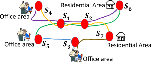
Figure 1: Illustration of the need of trajectory-aware querying for optimal locations. Each line represents a separate user trajectory.

With growing applications of data-driven location-based systems, the importance of OL queries is well-recognized in the database community [45, 40, 11]. However, most of the existing works assume the users to be fixed or static. Such an assumption is often too prohibitive. For example, services such as gas stations, ATMs, bill boards, traffic monitoring systems, etc. are widely accessed by users while commuting. Further, it is common for many users to make their daily purchases while returning from their offices. Consequently, the placement of facilities for these services require taking into consideration the mobility patterns (or trajectories) of the users rather than their static locations. We refer to such services as trajectory-aware services. Formally, a trajectory is a sequence of location-time coordinates that lie on the path of a moving user. Note that trajectories strictly generalize the static users’ scenario because static users can always be modeled as trajectories with a single user location. Thus, trajectories capture user patterns more effectively. Such trajectory data are commonly available from GPS traces [20] or CDR (Call Detail Records) data [25] recorded through cellphones, social network check-ins, etc. Recently, there have been many works in the area of trajectory data analytics [38, 23, 39, 16, 9, 27, 22, 21, 30].

To illustrate the need for trajectory-aware optimal location queries, consider Fig. 1. There are 5 locations that are either homes or offices and 5 trajectories of users commuting across them. A company wants to open 2 new gas stations. For simplicity, we assume that a trajectory of a user is satisfied if it passes through at least one gas station. If only the static locations are considered, i.e., any two out of the five office and residential areas are to be selected, no combination of gas stations would satisfy all the users. In contrast, if we factor in the mobility of the users, choosing $S_{1}$ and $S_{3}$ as the installation locations satisfies all the trajectories of the users.

Note that it is not enough to simply look at trajectory counts in each possible installation location and then choose the two most frequent ones ($S_{1}$ and $S_{2}$). The combination may not be effective since a large number of trajectories between them can be common, thereby reducing each other’s utilities.

In this work, we formalize the problem of OL queries over trajectories of users in road networks. We refer to this as TOPS (Trajectory-aware Optimal Placement of Services) query. Given a set of user trajectories $\mathcal{T}$, and a set of candidate sites $\mathcal{S}$ over a road network that can host the services, TOPS query with input parameters $k$ and preference function $\psi$ seeks to report the best $k$ sites $\mathcal{Q}\subseteq\mathcal{S}$ maximizing a utility function that is defined over the preference function $\psi$ which captures how a particular candidate site is preferred by a given trajectory.

Facility location queries with respect to trajectories have been studied by a number of previous works [7, 5, 2, 4, 3, 28]. Although the formulations are not identical, the common eventual goal is to identify the best sites. However, all these works remain limited to a theoretical exercise and cannot be applied in a real-life scenario due to a number of issues as explained next.

$\bullet$ Data-based mobility model: Existing techniques are neither based on real trajectories nor on real road networks [7, 5, 2, 4, 3]. They base their solutions on simplistic assumptions such as traveling in shortest paths and synthetic road networks. It is well known that the shortest path assumption does not hold in real life [1]. In many works, the distances are not computed over the road network but approximated using some spatial distance measure such as $L_{2}$ norm. Our framework is the first to study TOPS on real trajectories over real road networks.

$\bullet$ Generic framework: We develop the first generic framework to answer TOPS queries across a wide family of preference functions $\psi$ that are non-increasing w.r.t. the distance between any pair of trajectory and candidate site. The proposed framework encompasses many of the existing formulations and also considers other practical factors such as capacity constraints, site-costs, dynamic updates, etc.

$\bullet$ Scalability: The state-of-the-art technique for a basic version of TOPS query [2] requires prohibitively large memory. Consequently, it fails to scale on urban-scale datasets (Further details in Sec. 8). Hence, a scalable framework for TOPS query is a basic necessity. In addition, all OL queries including TOPS are typically used in an interactive fashion by varying the various parameters such as $k$ and the coverage threshold $\tau$ [11]. Moreover, in certain ventures, such as deployment of mobile ATM vans(https://goo.gl/WjSPvx), real-time answers are need based on current trajectory patterns. Hence, practical response time with the ability to absorb data updates is critical. This factor has been completely ignored in the existing works.

$\bullet$ Extensive benchmarking: Since TOPS queries and their variants are NP-hard, heuristics have been proposed. How do their effectiveness vary across road-network topologies? Are these heuristics biased towards certain specific parameter settings? The existing techniques are generally silent on these questions. We, on the other hand, perform benchmarking that is grounded to reality by extensively studying the performance of TOPS across multiple major city topologies and other important parameters.

To summarize, the proposed framework is the first practical and generic solution to address TOPS queries. Fig. 2 depicts the top-level flow diagram of our solution. Given the raw GPS traces of user movements, they are map-matched [33] to the corresponding road network. Using the map-matched trajectories, a multi-resolution clustering of the road network is built to construct the index structure NetClus. Indexed views of both the candidate sites and the trajectories are maintained in a compressed format at various granularities. This completes the offline phase. In the online phase, given the query parameters, the optimum clustering resolution to answer the query is identified, and the corresponding views of the trajectories and road network are analyzed to retrieve the best $k$ sites for facility locations.

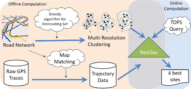
Figure 2: Flowchart of TOPS querying framework.

The major contributions of our work are as follows:

1. We propose a highly generic trajectory-aware optimal placement of services problem, TOPS, that can handle the wide class of preference functions $\psi$ that are non-increasing w.r.t. the distance between any pair of trajectory and candidate site (Sec. 2).

2. TOPS is NP-hard, and even the greedy approach does not scale in city-scale datasets (Sec. 3). To overcome this bottleneck, we design a multi-resolution clustering-based index structure called NetClus that generates a compressed representation of the road network and the set of trajectories (Sec. 4 and Sec. 5). The solutions returned by NetClus framework have bounded quality guarantees.

3. The proposed TOPS formulation is capable of absorbing dynamic updates (Sec. 6) and manage realistic constraints such as cost, capacity, and existing services. (Sec. 7).

4. Extensive experiments on real datasets show that NetClus offers solutions that are comparable in terms of quality with those of the greedy heuristic, while having practical response times and fairly low memory footprints (Sec. 8).

2 The TOPS Problem

Symbol	Description
$G=(V,E)$, $|V|=N$	Road network $G$ with node set $V$ and edge set $E$
$\mathcal{T}$, $|\mathcal{T}|=m$	Set of trajectories
$\mathcal{S}$, $|\mathcal{S}|=n$	Set of candidate sites
$d(u,v)$	Distance of shortest path from node $u$ to $v$
$d_{r}(u,v)$	Round-trip distance between nodes $u$ and $v$
$d_{r}(T_{j},s_{i})$	Round-trip distance from trajectory $T_{j}$ to site $s_{i}$
$k$	Desired number of service locations
$\tau$	Coverage threshold
$\psi(T_{j},s_{i})$	Preference function for trajectory $T_{j}$ and site $s_{i}$
$\mathcal{Q}\subseteq\mathcal{S}$, $|\mathcal{Q}|=k$	Set of locations to set up service
$U_{j}$	Utility of trajectory $T_{j}$ over the set of sites $\mathcal{Q}$
$U(\mathcal{Q})=\sum_{j=1}^{m}U_{j}$	Total utility offered by $\mathcal{Q}$

Table 1: Symbols used in the paper.

Consider a road network $G=\{V,E\}$ over a geographical area where $V$ denotes the set of road intersections, and $E$ denotes the set of road segments between two adjacent road intersections. The direction of the underlying traffic that passes over a road segment is modeled by directed edges.

Assume a set of candidate sites $\mathcal{S}=\{s_{1},\cdots,s_{n}\}\subseteq V$ where a certain service or facility can be set up. The choice of $\mathcal{S}$ is generally provided by the application itself by taking into account various factors such as availability, reputation of neighborhood, price of land, etc. Most of these factors are outside the purview of the main focus of this paper and are, therefore, not studied. We simply assume that the set $\mathcal{S}$ is provided as input to our problem. However, as described later, if all the latent factors of choosing a site can be encapsulated as its cost, we can handle it quite robustly.

The candidate sites can be located anywhere on the road network. If it is already on a road intersection, then it is part of the set of vertices $V$. If not, i.e., if it is on the middle of a road connecting vertices $u$ and $v$, without loss of generality, we augment $V$ to include this site as a new vertex $w$. We augment the edge set $E$ by two new edges $(u,w)$ and $(v,w)$ (with appropriate directions) and remove the old edge $(u,v)$. Thus, ultimately, $\mathcal{S}\subseteq V$.

The set of candidate sites $\mathcal{S}$ can be in addition to the set of existing service locations $\mathcal{E_{S}}$.

The set of trajectories over the road network is denoted by $\mathcal{T}=\{T_{1},\cdots,T_{m}\}$ where each trajectory is a sequence of nodes, $T_{j}=\{v_{j_{1}},\cdots,v_{j_{l}}\}$, $v_{j_{i}}\in V$. The trajectories are usually recorded as GPS traces and may contain arbitrary spatial points on the road network. For our purpose, each trajectory is map-matched [33] to form a sequence of road intersections through which it passes. We assume that each trajectory belongs to a separate user. However, the framework can easily generalize to multiple trajectories belonging to a single user by taking union of each of these trajectories.

Suppose $d(v_{i},v_{j})$ denotes the shortest network distance along a directed path from node $v_{i}$ to $v_{j}$, and $d_{r}(v_{i},v_{j})$ denotes the shortest distance of a round-trip starting at node $v_{i}$, visiting $v_{j}$, and finally returning to $v_{i}$, i.e., $d_{r}(v_{i},v_{j})=d(v_{i},v_{j})+d(v_{j},v_{i})$. In general, $d(v_{i},v_{j})\neq d(v_{j},v_{i})$, but $d_{r}(v_{i},v_{j})=d_{r}(v_{j},v_{i})$. With a slight abuse of notation, assume that $d_{r}(T_{j},s_{i})$ denotes the extra distance traveled by the user on trajectory $T_{j}$ to avail a service at site $s_{i}$. Formally, $d_{r}(T_{j},s_{i})=\min_{\forall v_{k},v_{l}\in T_{j}}\{d(v_{k},s_{i})+d(s_{i},v_{l})-d(v_{k},v_{l})\}$.

It is convenient for a user to avail a service only if its location is not too far off from her trajectory. Thus, beyond a distance $\tau$, we assume that the utility offered by a site $s_{i}$ to a trajectory $T_{j}$ is $0$. We call this user-specified distance $\tau$ as the coverage threshold.

Definition 1 (Coverage)

A candidate site $s_{i}$ covers a trajectory $T_{j}$ if the distance $d_{r}(T_{j},s_{i})$ is at most $\tau$, where $\tau\geq 0$ is the coverage threshold.

For all sites within the coverage threshold $\tau$, the user also specifies a preference function $\psi$. The preference function $\psi(T_{j},s_{i})$ assigns a score (normalized to $[0,1]$) for a trajectory $T_{j}$ and a site $s_{i}$ that indicates how much $s_{i}$ is preferred by the user on trajectory $T_{j}$. Higher values indicate higher preferences with $0$ indicating no preference. In general, sites that are closer to the trajectory have higher preferences than those farther away. Usage of such preference functions are common in location analysis literature [44].

Definition 2 (Preference Function $\psi$)

$\psi:(\mathcal{T},\mathcal{S})\rightarrow[0,1]$ is a real-valued preference function defined as follows:

$$\psi(T_{j},s_{i})=\begin{cases}f(d_{r}(T_{j},s_{i}))&\text{ if }d_{r}(T_{j},s_{i})\leq\tau\\ 0&\text{otherwise}\end{cases}$$ (1)

where $f$ is a non-increasing function of $d_{r}(T_{j},s_{i})$.

Trajectories	Preference scores for different sites
	$s_{1}$	$s_{2}$	$s_{3}$
$T_{1}$	$\psi(T_{1},s_{1})=0.4$	$\psi(T_{1},s_{2})=0.11$	$\psi(T_{1},s_{3})=0$
$T_{2}$	$\psi(T_{2},s_{1})=0$	$\psi(T_{2},s_{2})=0.5$	$\psi(T_{2},s_{3})=0.6$

Table 2: Examples of trajectories with site preferences.

The goal of TOPS query is to report a set of $k$ sites $\mathcal{Q}\subseteq\mathcal{S},\ |\mathcal{Q}|=k$, that maximizes the preference score over the set of trajectories. The preference score of a trajectory $T_{j}$ over a set of sites $\mathcal{Q}$ is defined as the utility function $U_{j}$ for $T_{j}$, which is simply the maximum score corresponding to the sites in $\mathcal{Q}$, i.e., $U_{j}=\max_{s_{i}\in\mathcal{Q}}\{\psi(T_{j},s_{i})\}$. The various symbols used in the TOPS formulation are listed in Table 1.

The generic TOPS query formulation is stated next.

Problem 1 (TOPS)

Given a set of trajectories $\mathcal{T}$, a set of candidate sites $\mathcal{S}$ that can host the services, TOPS problem with query parameters $(k,\tau,\psi)$ seeks to report the best $k$ sites, $\mathcal{Q}\subseteq\mathcal{S},\ |\mathcal{Q}|=k$, that maximize the sum of trajectory utilities, i.e., $\mathcal{Q}=\arg\max\sum_{j=1}^{m}U_{j}$ where $U_{j}=\max_{s_{i}\in Q}\{\psi(T_{j},s_{i})\}$.

Extensions and variants of TOPS: The TOPS framework as defined above is generic. It can have various extensions as described in Sec. 7.1 and Sec. 7.2 and can work with existing facilities as well (Sec. 7.3). Finally, the preference function in Def. 2 subsumes various existing models as exemplified in Sec. 7.4.

2.1 Properties of TOPS

TOPS problem is NP-hard. To show that, we first define a specific instance of TOPS where the preference function $\psi(T_{j},s_{i})$ is a binary function. A binary function is a natural choice in situations where a service provider wants to intercept the maximum number of trajectories that pass within a vicinity of it [2].

Definition 3 (Binary Instance of TOPS)

TOPS with parameters $(k,\tau,\psi)$ where the preference score is given by:

$$\psi(T_{j},s_{i})=\begin{cases}1&\text{ if }d_{r}(T_{j},s_{i})\leq\tau\\ 0&\text{otherwise}\end{cases}$$ (2)

Theorem 1

TOPS is NP-hard.

Proof 2.1.

This follows from the fact that the binary instance of TOPS is NP-hard, as set cover problem is reducible to it [2].

Next we show that the sum of utilities $U=\sum_{j=1}^{m}U_{j}$ is a non-decreasing sub-modular function. A function $f$ defined on any subset of a set $\mathcal{S}$ is sub-modular if for any pair of subsets $\mathcal{Q,R}\subseteq\mathcal{S}$, $f(\mathcal{Q})+f(\mathcal{R})\geq f(\mathcal{Q}\cup\mathcal{R})+f(\mathcal{Q}\cap\mathcal{R})$ [37].

Theorem 2.

$U=\sum_{j=1}^{m}U_{j}$ is non-decreasing and sub-modular.

Proof 2.2.

Consider any two pair of subsets $\mathcal{Q,R}\subseteq\mathcal{S}$ such that $\mathcal{Q}\subseteq\mathcal{R}$. Since $U_{j}=\max_{s_{i}\in\mathcal{Q}}\{\psi(T_{j},s_{i})\}$, $U_{j}(\mathcal{R})\geq U_{j}(\mathcal{Q})$. Therefore, $\sum_{j=1}^{m}U_{j}(\mathcal{R})=U(\mathcal{R})\geq\sum_{j=1}^{m}U_{j}(\mathcal{Q})=U(\mathcal{Q})$. Hence, $U$ is a non-decreasing function.

To show that $U$ is sub-modular, following [37], it is sufficient to show that for any two subsets $\mathcal{Q,R}\subseteq\mathcal{S},\ \mathcal{Q}\subset\mathcal{R}$, for any site $s\in\mathcal{S}\setminus\mathcal{R}$, $U(\mathcal{Q}\cup\{s\})-U(\mathcal{Q})\geq U(\mathcal{R}\cup\{s\})-U(\mathcal{R})$. For our formulation, it is, thus, enough if for any trajectory $T_{j}\in\mathcal{T}$,

$$U_{j}(\mathcal{Q}\cup\{s\})-U_{j}(\mathcal{Q})\geq U_{j}(\mathcal{R}\cup\{s\})-U_{j}(\mathcal{R})$$ (3)

Suppose the site $s^{*}\in\mathcal{R}\cup\{s\}$ offers the maximal utility to trajectory $T_{j}$ in the set of sites $\mathcal{R}\cup\{s\}$. There can be two cases:
(a) $s^{*}=s$: $U_{j}(\mathcal{Q}\cup\{s\})=U_{j}(\{s\})=U_{j}(\mathcal{R}\cup\{s\})$. Further, $U_{j}(\mathcal{Q})\leq U_{j}(\mathcal{R})$ since $U_{j}=\{\max\{\psi(T_{j},s_{i})\}|s_{i}\in Q\}$. These two inequalities together lead to Ineq. (3).
(b) $s^{*}\neq s$: Here, $U_{j}(\mathcal{R}\cup\{s\})-U_{j}(\mathcal{R})=0$. As $U_{j}()$ is non-decreasing, $U_{j}(\mathcal{Q}\cup\{s\})\geq U_{j}(\mathcal{Q})$. Thus, Ineq. (3) follows.

3 Algorithms for TOPS

Algorithm	Selected sites $\mathcal{Q}$	Utility $U$
Optimal	$\{s_{1},s_{3}\}$	$1.0$
Inc-Greedy	$\{s_{1},s_{2}\}$	$0.9$

Table 3: Utilities of different algorithms for Example 3.1 with $k=2$.

We first state an example, using which we will explain the different algorithms for TOPS problem.

Example 3.1.

Consider Table 2, which lists $2$ trajectories $T_{1},T_{2}$ with their preference scores for $3$ sites $s_{1}$, $s_{2}$ and $s_{3}$. We set $k=2$ sites to be selected for TOPS query. The utilities achieved by different algorithms (discussed next) are shown in Table 3. The optimal solution consists of the sites $s_{1}$ and $s_{3}$ with a total utility of $1.0$.

3.1 Optimal Algorithm

We first discuss the optimal solution to TOPS problem in the form of an integer programming problem (ILP):

$$\text{Maximize }U =\sum_{j=1}^{m}U_{j}$$ (4)

$$\text{such that }\sum_{i=1}^{n}x_{i} \leq k,$$ (5)

$$\forall j=1,\dots,m,\ U_{j} \leq\max_{1\leq i\leq n}\{\psi(T_{j},s_{i})\times x_{i}\}$$ (6)

$$\forall i=1,\dots,n,\ x_{i} \in\{0,1\}$$ (7)

The above IP is, however, not in the form of a standard integer linear program (ILP). To do so, the constraints in Ineq. (6) can be linearized, as discussed in Appendix A.1. Since TOPS is NP Hard, the cost of solving this optimal algorithm is exponential with respect to the number of trajectories $m$, and the number of sites $n$ and, therefore, impractical except for very small $m$ and $n$. This is demonstrated through experiments in Sec. 8.3.

3.2 Approximation Algorithms

We next present a greedy approximation algorithm. Before that, let us define a few terms and how they are computed.

Given a site $s_{i}\in\mathcal{S}$, $TC(s_{i})$ denotes the set of trajectories covered by $s_{i}$, i.e., $TC(s_{i})=\{T_{j}|d_{r}(T_{j},s_{i})\leq\tau\}$. Similarly, given a trajectory $T_{j}$, $SC(T_{j})$ denotes the set of sites that cover $T_{j}$, i.e., $SC(T_{j})=\{s_{i}|d_{r}(T_{j},s_{i})\leq\tau\}$. For each site $s_{i}$, the site weight $w_{i}=\sum_{j=1}^{m}\{\psi(T_{j},s_{i})|T_{j}\in TC(s_{i})\}$ denotes the sum of preference scores of all the trajectories covered by it. Table 4 tabulates some of the important notations.

Since $\tau$ is available only at query time, the computation of these covering sets need to be efficient. Hence, for each site $s_{i}\in\mathcal{S}$, the shortest path distances to all other nodes in $V$ are pre-computed. This requires $O(|\mathcal{S}|.|E|\log|V|)$ time [12]. As the road network graphs are almost planar, i.e., $|E|=O(|V|)$, the above cost simplifies to $O(n.N\log N)$ where $n=|\mathcal{S}|$ and $N=|V|$.

Using these distance values, the distance between each pair of site and trajectory, $d_{r}(T_{j},s_{i})$, is computed. Suppose there are at most $l$ nodes in a trajectory $T_{j}$, i.e., $\max_{T_{j}\in\mathcal{T}}|T_{j}|=l$. Referring to the definition of $d_{r}(T_{j},s_{i})$ in Sec. 2, it follows that $d_{r}(T_{j},s_{i})$ can be computed in $O(l^{2})$ time for a given site-trajectory pair using the above site-node distances. Therefore, the total cost across all $n$ sites and $m$ trajectories is $O(mnl^{2})$.

Each site $s_{i}$ maintains the set of trajectories in an ascending order of $d_{r}(T_{j},s_{i})$ while each trajectory $T_{j}$ maintains the sites in a similar ascending order based on $d_{r}(T_{j},s_{i})$ again. Sorting increases the time to $O(mn(\log n+\log m))$. The space complexity for storing all site to trajectory distances is $O(mn)$.

At query time, when $\tau$ is available, the sets $TC$, $SC$, and the site weights can be, thus, computed from the stored distance matrix in $O(mn)$ time.

Alternatively, the sets $TC$ and $SC$ can be computed at query time when $\tau$ is made available. However, for a city-sized road network, even a small $\tau$ includes a lot of neighbors (e.g., for the Beijing dataset described in Sec. 8, there are more than $40$ sites on average within a distance of $\tau=0.8$ Km from a site). Since this needs to be computed for all the candidate sites, this approach is infeasible at query time.

3.3 Inc-Greedy

We adapt the general greedy heuristic for maximizing non-decreasing sub-modular functions [37] to design Inc-Greedy. The main idea is based on the principle of maximizing marginal gain.

Then the algorithm starts with an empty set of sites $\mathcal{Q}_{0}=\varnothing$, and incrementally adds the sites (one in each of the $k$ iterations) such that each successive addition of a site produces the maximal marginal gain in the utility $U$. More specifically, if the set of selected sites after $\theta-1$ iterations $(\theta=1,\dots,k)$ is $\mathcal{Q}_{\theta-1}=\{s_{1},\dots,s_{\theta-1}\}$, in the $\theta^{th}$ iteration, Inc-Greedy chooses the site $s_{\theta}\notin\mathcal{Q}_{\theta-1}$ such that $U(\mathcal{Q}_{\theta}=\mathcal{Q}_{\theta-1}\cup\{s_{\theta}\})-U(\mathcal{Q}_{\theta-1})$ is maximal.

The marginal utility gained due to the addition of $s_{i}$ to the set $\mathcal{Q}_{\theta-1}$ in iteration $\theta=1,\dots,k$ is $U_{\theta}(s_{i})=U(\mathcal{Q}_{\theta-1}\cup\{s_{i}\})-U(\mathcal{Q}_{\theta-1})$. Thus, $U(\mathcal{Q}_{\theta})=\sum_{i=1}^{\theta}U_{i}(s_{i})$. If $\alpha_{ji}$ denotes the marginal gain in the utility of trajectory $T_{j}$ by addition of site $s_{i}$ to the existing set of chosen sites, then, at the end of each iteration $\theta=1,\dots,k$, $U_{\theta}(s_{i})=\sum_{\forall T_{j}\in TC(s_{i})}\alpha_{ji}$.

Inc-Greedy algorithm begins by computing the sets $TC,SC$, and the site-weights as explained above. It then initializes the marginal utilities of each site $s_{i}\in\mathcal{S}$ to its site weight, i.e., $U_{1}(s_{i})=w_{i}$. Further, for each trajectory $T_{j}\in TC(s_{i})$, it initializes $\alpha_{ji}=\psi(T_{j},s_{i})$.

In iteration $\theta=1,\dots,k$, it selects the site $s_{\theta}$ with maximal marginal utility, i.e., $\forall s_{i}\notin\mathcal{Q}_{\theta-1},U_{\theta}(s_{\theta})\geq U_{\theta}(s_{i})$. If multiple candidate sites yield the same maximal marginal gain, it chooses the one with maximal weight. Still, if there are ties, then without loss of generality, the site with the highest index is selected.

For each trajectory $T_{j}\in TC(s_{\theta})$, first the utility $U_{j}$ is updated as follows: $U_{j}\leftarrow\max(U_{j},\psi(T_{j},s_{\theta}))$. In case there is a gain in $U_{j}$, the marginal utility of each site $s_{i}\in SC(T_{j})$ is updated.

The pseudocode of Inc-Greedy is prsented in Appendix A.2.

In Example 3.1, at iteration $1$, the site $s_{2}$ has the largest marginal utility of $0.61$ and is, therefore, selected. With $\mathcal{Q}_{1}=\{s_{2}\}$, the marginal utility of adding the site $s_{1}$ is $0.4-0.11=0.29$, and that of site $s_{3}$ is $0.6-0.5=0.1$. Hence, Inc-Greedy selects the sites $s_{1}$ and $s_{2}$, and yields an utility $U=0.9$, as indicated in Table 3.

We next analyze the quality of Inc-Greedy.

Lemma 3.

The approx. bound of Inc-Greedy is $(1-1/e)$.

Proof 3.2.

Since Inc-Greedy is a direct adaptation of the generic greedy algorithm for maximizing non-decreasing sub-modular functions under cardinality constraints [37] with $U(\varnothing)=0$, it offers the approximation bound of $\left(1-(1-\frac{1}{k})^{k}\right)\geq\left(1-\frac{1}{e}\right)$.

Lemma 4.

$U(\mathcal{Q}_{k})\geq(k/n).U(\mathcal{S})$.

Proof 3.3.

From Theorem 2 it follows that successive marginal utilities are non-increasing, i.e., $U_{\theta}(s_{\theta})\geq U_{\theta+1}(s_{\theta+1})$. Thus,

$$U_{\theta}(s_{\theta})\geq\frac{\sum_{i=\theta}^{n}U_{i}(s_{i})}{n-\theta+1}\geq\frac{U(\mathcal{Q}_{n})-U(\mathcal{Q}_{\theta-1})}{n-\theta+1}$$ (8)

Next, we claim that $\forall\theta=1,2,\dots,n$,

$$U(\mathcal{Q}_{\theta})\geq(\theta/n).U(\mathcal{Q}_{n})$$

We will prove this by induction on $\theta$.

Consider the base case $\theta=1$. Using Ineq. (8), $U(\mathcal{Q}_{1})=U_{1}(s_{1})\geq U(\mathcal{Q}_{n})/n$ since $U(\mathcal{Q}_{0})=0$. Thus, the induction hypothesis is true for the base case.

Next, we assume it to be true for iteration $\theta$. For iteration $\theta+1$,

$$U(\mathcal{Q}_{\theta+1}) =U(\mathcal{Q}_{\theta})+U_{\theta+1}(s_{\theta+1})$$

$$\geq U(\mathcal{Q}_{\theta})+\frac{U(\mathcal{Q}_{n})-U(\mathcal{Q}_{\theta})}{n-\theta}$$

$$\geq\left(\frac{n-\theta-1}{n-\theta}\right)U(\mathcal{Q}_{\theta})+\left(\frac{1}{n-\theta}\right)U(\mathcal{Q}_{n})$$

Using the induction hypothesis for iteration $\theta$,

$$U(\mathcal{Q}_{\theta+1}) \geq\left(\frac{n-\theta-1}{n-\theta}\right)\left(\frac{\theta}{n}\right)U(\mathcal{Q}_{n})+\left(\frac{1}{n-\theta}\right)U(\mathcal{Q}_{n})$$

$$\geq\left(\frac{\theta+1}{n}\right).U(\mathcal{Q}_{n})$$

Thus, the induction hypothesis holds true for any $\theta=1,\dots,n$.

Since $\mathcal{Q}_{n}=\mathcal{S}$, after $k$ iterations, $U(\mathcal{Q}_{k})\geq(k/n).U(\mathcal{S})$.

Lemma 5.

The approximation bound of Inc-Greedy is $(k/n)$.

Proof 3.4.

Since $U$ is non-decreasing (from Th. 2) and $OPT\subseteq\mathcal{S}$, therefore $U(OPT)\leq U(\mathcal{S})$. The rest follows from Lem. 4.

Theorem 6.

The approximation bound of Inc-Greedy for TOPS is $\max\{1-1/e,k/n\}$.

Proof 3.5.

The result follows from Lem. 3 and Lem. 5.

The next result establishes the complexity of Inc-Greedy.

Theorem 7.

The time and space complexity bounds for Inc-Greedy are $O(k.mn)$ and $O(mn)$ respectively.

Proof 3.6.

As discussed earlier in Sec. 3.2, the computation of the sets $TC$, $SC$ and the weights require $O(mn)$ time and storage.

Initializing the marginal utilities $U_{\theta}(s_{i})$ of all the sites and $\alpha_{ji}$ values for all trajectory site pairs require $O(mn)$ time.

In any iteration $\theta=1,\dots,k$, selecting the site with maximal marginal utility requires at most $O(n)$ time. The largest size of any $TC$ set is at most $m$ and that of any $SC$ set is at most $n$. Hence, scanning the set of trajectories $TC(s_{\theta})$ and updating the utilities requires $O(m)$ time. If $U_{j}$ gets updated, then scanning the set of sites in $SC(T_{j})$ and updating the values of $U_{\theta}(s_{i})$ and $\alpha_{ji}$ requires $O(n)$ time. Thus, the time complexity of any iteration $\theta$ is $O(mn)$. Hence, the total time complexity of $k$ iterations is $O(kmn)$.

Since no other space is required than that for storing $TC$, $SC$ and site weights, the total space complexity is $O(mn)$.

3.4 Limitations of Inc-Greedy

Although Inc-Greedy provides a constant factor approximation, it is not scalable to large real-life datasets. The reasons are:

High query cost: The input parameters for TOPS query, $(k,\tau,\psi)$, are available only at query time. Hence, the covering sets $TC$, $SC$, and the site weights (that depend on the value of $\tau$) can be generated only at query time. Even if all pairwise site-to-trajectory distances are pre-computed, this step requires a high computation cost of $O(mn)$ (both in terms of time and memory) where $m,n$ denote the number of trajectories, and candidate sites, respectively. Due to this reason, for real city-scale datasets (such as the Beijing dataset [42] used in our experiments that has over 120,000 trajectories and 250,000 sites), Inc-Greedy is not scalable. Fig. 6b shows that Inc-Greedy takes about 2000 sec. to complete for $\tau=1.2$ Km. and $k=5$, and goes out of memory for $\tau>1.2$ Km.

High storage cost: As discussed above, to facilitate faster computation of covering sets $TC$, we need to pre-compute all pairwise site-to-trajectory distances. However, for any city-scale dataset, this storage requirement is prohibitively large. For example, the Beijing dataset [42] require close to 250 GB of storage. This is unlikely to fit in the main memory and, therefore, multiple expensive random disk seeks are required at run-time. Even with pre-computed distances up to 10 Km., Inc-Greedy crashes beyond $\tau\>1.2$ Km. (shown in Tab. 9.)

High update cost: Inc-Greedy is also not amenable to updates in trajectories and sites. If a new trajectory is added, its distance to all the sites needs to be computed and sorted. In addition, the sorted $TC$ set of all the sites need to be updated as well. Similarly, if a new candidate site is added, the distances of all the trajectories to this site will need to be computed and sorted. Such costly update operations are impractical, especially at run-time.

A careful analysis of Inc-Greedy reveals that there are two main stages of the algorithm. In the first, the sets $TC$, $SC$ and the site weights are computed. In the second stage, some of these sets are updated in an iterative manner.

The first stage is heavier in terms of time and space requirements. Thus, to make it efficient, we use an index structure, NetClus, which is described in Sec. 4 and Sec. 5. The use of indexing reduces the computational burden of the update (i.e., the second) stage as well. Further, Section 6 shows how NetClus allows easier handling of additions and deletions of candidate sites and trajectories.

In addition, if the preference function $\psi$ is binary as defined in Def. 3, the update steps for Inc-Greedy can be performed quite efficiently using FM sketches [15, 32]. We next describe the details.

3.5 Using FM Sketch to speed up Inc-Greedy

The main use of FM sketches is in counting the number of distinct elements in a set or union of sets [15]. Suppose, the maximum number of distinct elements is $N$. An FM sketch is a bit vector, which is initially empty, and is of size at least $O(\log_{2}N)$. The probability of an element from the domain hashing into the $i^{\text{th}}$ bit of the FM sketch is $2^{-i}$. Thus, if a set has $\Gamma$ elements, the probability of the last bit marked in the FM sketch is $O(\log_{2}\Gamma)$. Hence, after the elements of a set are hashed to the FM sketch, the last set bit can be used to estimate the number of distinct elements in the set. (The details of how the hashing function is chosen and the exact estimates are in [15].) Although the FM sketch does not count the number of distinct elements exactly, it provides a multiplicative guarantee on the error in counting. When more copies of the FM sketch is used, the error decreases.

The FM sketch can be used to speed up the update stage of Inc-Greedy, since selecting a site with the largest maximal utility is the same as selecting a site that covers the largest number of distinct trajectories not yet covered.

For each site $s_{i}\in\mathcal{S}$, the set of trajectories that it covers, i.e., $TC(s_{i})$ is maintained as an FM sketch. Thus, instead of maintaining $O(m)$-sized lists for each site where $m$ is the total number of trajectories, we only need to maintain $O(\log_{2}m)$-sized bit vectors per site.

Suppose the count of distinct trajectories covered by a site $s_{i}$ is $\chi_{i}$. The marginal utility of site $s_{j}$ when site $s_{i}$ has been chosen is the number of distinct trajectories that the two sites together cover over the number of trajectories that site $s_{i}$ alone covers. The estimate of the number of trajectories covered by the union of $s_{j}$ and $s_{i}$ can be obtained by the bitwise OR of the FM sketches corresponding to $s_{j}$ and $s_{i}$. If this estimate is $\chi_{ij}$, the marginal utility of site $s_{j}$ over site $s_{i}$ is $\chi_{ij}-\chi_{i}$.

Therefore, when there are $n$ candidate sites, to determine the site that provides the best marginal utility over site $s_{i}$, $n-1$ such bitwise OR operations are performed, and the maximum is chosen. At the end of the $\theta^{\text{th}}$ iteration, the combined number of trajectories covered by the sites in $\mathcal{Q}_{\theta}$ is stored by the union of the FM sketches obtained successively in the $\theta$ iterations. The $(\theta+1)^{\text{th}}$ site is chosen by using this combined FM sketch as the base.

The above brute-force algorithm can be improved in the following way. The upper bound of the marginal utility for any site $s_{j}$ is its own utility. Thus, if the current best marginal utility of another site $s_{k}$ is already greater than that, it is not required to do the union operation with $s_{j}$. If the sites are sorted according to their utilities, the scan can stop as soon as the first such site $s_{j}$ is encountered. All sites having a lower utility are guaranteed to be useless as well.

In our implementation, the FM sketches are stored as $32$-bit words. This allows handling of roughly $2^{32}$ (which is more than $4$ billion) number of trajectories. The length $32$ is chosen since the bitwise OR operation of two such regular-sized words is extremely fast in modern operating systems.

4 Offline Construction of NetClus

As discussed in Sec. 3.4, Inc-Greedy has two computationally expensive components. While FM sketch expedites the information update component, computation of $TC$, $SC$, etc. still remain a bottleneck with $O(mn)$ time and storage complexity. To overcome this scalability issue, we develop an index structure.

One of the most natural ways to achieve the above objectives is to cluster the sites in the road network to reduce the number, and then apply Inc-Greedy on the cluster representatives. The clustering of sites can be done according to two broad strategies. The first is to cluster the sites that are highly similar in terms of their trajectory covering sets $TC$. The similarity between these covering sets can be quantified using the Jaccard similarity measure (Appendix B.1). However, this approach is not practical due to two major limitations: (1) Since the coverage threshold $\tau$ is available only at query time, the covering sets $TC$ can be computed only at query time. Hence, the clustering can be performed only at query time. This leads to impractical query time. (2) Alternatively, multi-resolution clustering may be performed based on few fixed values of $\tau$, and at query time, a clustering instance of a particular resolution is chosen based on the value of the query parameter $\tau$. However, this still requires computing the similarity between each pair of sites. Owing to large number of sites, and large size of the covering sets, such computation demands impractical memory overhead. Hence, we adopt the second clustering option, that of distance-based clustering.

We first state one basic observation. If two sites are close, the sets of trajectories they cover are likely to have a high overlap. Hence, when $k\ll n$, which is typically the case, the sites chosen in the answer set are likely to be distant from each other. The index structure, NetClus, is designed based on the above observation.

Our method follows two main phases: offline and online. In the offline phase, clusters are built at multiple resolutions. This forms the different index instances. A particular index instance is useful for a particular range of query coverage thresholds. In the online phase, when the query parameters are known, first the appropriate index instance is chosen. Then the Inc-Greedy algorithm is run with the cluster representatives of that instance.

We explain the offline phase in this section and the online phase in the next. The important notations used in the NetClus scheme are listed in Table 4.

4.1 Distance-Based Clustering

The clustering method is parameterized by a distance threshold $R$, which is the maximum cluster radius. The round-trip distance from any node within the cluster to the cluster-center is constrained to be at most $2R$. The radius is varied to obtain clusters at multiple resolutions. We describe the significance of the choices of $R$ later.

The objective of the clustering algorithm is to partition the set of nodes in the road network, $V$, into disjoint clusters such that the number of such clusters is minimal. This leads not only to savings in index storage, but more importantly, it results in faster query time, as Inc-Greedy is run on a smaller number of cluster representatives. We next describe how to achieve this objective.

4.1.1 Generalized Dominating Set Problem (GDSP)

Given an undirected graph $G=(V,E)$, the dominating set problem (DSP) [19] computes a set $D\subseteq V$ of minimal cardinality, such that for each vertex $v\in V-D$, there exists a vertex $u\in D$, such that $(u,v)\in E$. DSP is NP-hard [19]. In [10], it was generalized to the measured dominating set problem for weighted graphs. In this work, we propose a generalized dominating set problem (GDSP), that uses a different notion of dominance from [10].

Problem 8 (GDSP).

Given a weighted directed graph $G=(V,E,W)$ where $W:E\rightarrow\mathbb{N}$ assigns a positive weight for each edge in $E$, and a constant $R>0$, a vertex $u\in V$ is said to dominate another vertex $v\in V$ if $d(u,v)+d(v,u)\leq 2R$, where $d$ denotes the directed path weight. The GDSP problem computes a set $D\subseteq V$ of minimal cardinality such that for any $v\in V-D$, there exists a vertex $u\in D$ such that $u$ dominates $v$.

GDSP is NP-hard due to a direct reduction from DSP where all edge weights are assumed to be $1$, and $R=2$.

4.1.2 Greedy Algorithm for GDSP

To solve GDSP, we adapt the greedy algorithm proposed in [10]. We refer to our algorithm as Greedy-GDSP. The only input parameter to the clustering process is the cluster radius $R$.

First, the dominating sets of every vertex $v$, denoted by $\Lambda(v)$, are computed. This is achieved by running the shortest path algorithm from a source vertex till distance $2R$. The dominance relationship is symmetric, i.e., $u\in\Lambda(v)\Leftrightarrow v\in\Lambda(u)$.

The main part of the Greedy-GDSP algorithm is iterative. In the first iteration, the vertex $v$ that dominates the largest number of vertices is chosen. The set of dominated vertices, $\Lambda(v)$, forms a new cluster with $v$ as the cluster center. The vertices $v$ and $\Lambda(v)$ are not considered for further comparisons. In addition, the vertices in $\Lambda(v)$ are removed from the dominating sets of other non-clustered vertices. In other words, for each $u\in\Lambda(v)$, if $u\in\Lambda(w)$ for some non-clustered vertex $w$ then $\Lambda(w)=\Lambda(w)-\{u\}$. In the subsequent iterations, the vertex with the largest incremental dominating set as produced from previous iterations is chosen. The dominated vertices that are not part of other clusters form a new cluster. The algorithm terminates when all the vertices are clustered.

Similar to the Inc-Greedy algorithm, we use FM sketches to efficiently update the dominating sets and choose the vertex with the largest incremental dominating set in each iteration. The details are same as those described in Sec. 3.5 with trajectory covering sets for each candidate site in Inc-Greedy replaced by dominating sets for each vertex in Greedy-GDSP.

4.1.3 Analysis of Greedy-GDSP

The next two theorems characterize the approximation bound and time complexity of Greedy-GDSP.

Theorem 9.

The cardinality of the dominating set computed using the proposed algorithm is within an approximation bound of $(1+\epsilon^{\prime}).(1+\ln n)$ of the optimal where $\epsilon^{\prime}$ is the approximation error of FM sketches.

Proof 4.1.

Following the analysis in [10], the Greedy-GDSP algorithm offers an approximation bound of $H_{n}=1+\frac{1}{2}+\dots+\frac{1}{n}\leq 1+\ln n$ which was shown to be tight unless $P=NP$. This, however, does not consider the approximation due to the use of FM sketches. Incorporating that, the bound becomes $(1+\epsilon^{\prime}).(1+\ln n)$ where $\epsilon^{\prime}$ is the approximation error of FM sketches.

Theorem 10.

Greedy-GDSP runs in $O(|V|.(\nu\log\nu+\eta))$ time where $\nu$ is the maximum number of vertices that are reachable within the largest round-trip distance $R_{max}$ from any vertex $v$, and $\eta$ is the number of clusters returned by the algorithm.

The proof is given in Appendix B.2.

Symbol	Description
$TC(s)$	Set of trajectories covered by site $s$
$\mathcal{CL}(g)$	Neighbors of cluster $g$
$\mathcal{TL}(g)$	Set of trajectories passing through cluster $g$
$TC(g)$	Set of trajectories passing through $g$ and its neighbors $\mathcal{CL}(g)$
$\widehat{d_{r}}(T,s)$	Estimate of $d_{r}(T,s)$ in the clustered space
$\widehat{TC}(s)$	Estimate of $TC(s)$ in the clustered space
$\gamma$	Resolution at which index instances change
$t$	Number of index instances
$p$	Index instance
$R_{p}$	Cluster radius for $p$
$\eta_{p}$	Number of clusters for $p$
$\Lambda(v)$	Dominating set for node $v$
$f$	Number of bit vectors for FM sketch
$\epsilon$	Error parameter for FM sketch

Table 4: Important notations used in the algorithms.

4.2 Selection of Cluster Representatives

In order to run Inc-Greedy on the clusters, each cluster needs to choose a representative candidate site. This may be different from the cluster center that was used to construct the cluster. The flexibility is needed since the cluster representative should necessarily be a candidate site, although the cluster center may be any vertex in $V$. Taking into account the fact that the cluster representative should summarize the information about the cluster and the trajectories that pass through it, and use this information to compete against the other cluster representatives in the online phase, we study two alternatives of choosing the cluster representative:

1. The most frequently accessed candidate site, i.e., the one through which the largest number of trajectories pass through.

2. The candidate site that is closest to the cluster center.

While the first option guarantees that the utility of the cluster is at least that of its best site, the second summarizes the distribution of trajectories better. Empirical studies show that the utilities returned by the two alternatives are quite similar, but the second alternative is marginally better. Consequently, we adopt the second option.

4.3 Cluster Information

Suppose the above clustering algorithm produces clusters of radius $R$, i.e., the maximum round-trip distance of any node within a cluster to its cluster center is at most $2R$. Then, a pair of clusters are considered as neighbors of each other if their centers are within a round-trip distance of $4.R(1+\gamma)$, where $\gamma\in(0,1]$ is the index resolution parameter to be described in Sec. 4.4. This choice of neighborhood is explained in Sec. 5.1.

As part of the index structure, every cluster $g_{i}$ stores the following information:

1. Cluster center, $c_{i}$.

2. Cluster representative, $r_{i}$.

3. Trajectory set, i.e., list of trajectories passing through at least one site in $g_{i}$, along with their round-trip distance to $c_{i}$, $\mathcal{TL}(g_{i})=\langle T_{j},d_{r}(T_{j},c_{i})\rangle$.

4. Cluster neighbors along with the round-trip distance between their centers and $c_{i}$, $\mathcal{CL}(g_{i})=\{\langle g_{j},d_{r}(c_{i},c_{j})\rangle\}$, sorted by $d_{r}(c_{i},c_{j})$.

5. Set of nodes in the cluster and their round-trip distance to $c_{i}$, $\{\langle v_{i},d_{r}(v_{i},c_{i})\rangle\}$.

The set $\mathcal{TL}(g_{i})$ is computed by scanning the sequence of nodes in each trajectory $T_{j}$. If $v_{i}\in T_{j}$, then $T_{j}$ is added to $\mathcal{TL}(g(v_{i}))$, where $g(v_{i})$ denotes the cluster in which $v_{i}$ resides. Thus, a trajectory is represented as a sequence of clusters. As neighboring nodes in any trajectory are likely to fall into the same cluster, this allows a compressed representation of the trajectory by collapsing consecutive copies of the same cluster into one. This compression contributes towards the efficiency of NetClus in terms of both space and time.

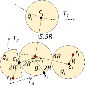
(a) Example

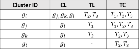
(b) Covering Sets

Figure 3: NetClus example using $\gamma=0.5$.

Example 4.2.

Fig. 3b illustrates an example of NetClus clustering with cluster radius $R$ and $\gamma=0.5$. The clusters $g_{i}$, $g_{j}$, $g_{k}$ and $g_{l}$ have centers $c_{i}$, $c_{j}$, $c_{k}$ and $c_{l}$ respectively. The cluster $g_{i}$ has two candidate sites $r_{i}$ and $s_{i}$. Since $r_{i}$ is located at $c_{i}$, it is chosen as the cluster-representative. While cluster $g_{j}$ has no candidate site, each of the clusters $g_{k}$ and $g_{l}$ have one candidate site, namely, $r_{k}$ and $r_{l}$, respectively, each of which is a cluster-representative. The distance between the cluster centers are as follows: $d_{r}(c_{i},c_{j})=5.5R$, $d_{r}(c_{i},c_{k})\gtrsim 2R$, and $d_{r}(c_{i},c_{l})=4R$ where $\gtrsim$ means just greater than. The distance between any other pair of cluster centers is greater than or equal to $6R$. Given that $\gamma=0.5$, the distance between any two neighboring cluster centers lies in the range $[2R,6R)$. Based on this, the cluster neighbors, $\mathcal{CL}$, are shown in the figure. The trajectories $T_{1}$, $T_{2}$ and $T_{3}$ pass through nodes $c_{j}$, $r_{i}$ and $s_{i}$, respectively. The figure lists the trajectory sets $\mathcal{TL}$ for each cluster. Note that when $\tau\geq 4R$, it is guaranteed that any site covers any trajectory that passes through the same cluster. For example, $r_{k}$ covers $T_{2}$ as it passes through the cluster $g_{k}$ that contains $r_{k}$. $\square$

4.4 Multi-Resolution Index Structure

We next explain how the multi-resolution index structure, NetClus, is built by using the clustering algorithm outlined above. Assume that the normal range of query coverage threshold $\tau$ is $[\tau_{min}$, $\tau_{max})$. (We discuss the two extreme cases later.) NetClus maintains $t$ instances of index structures $0,\dots,{t-1}$ of varying cluster radii. From one instance to the next, the radius increases by a factor of $(1+\gamma)$ for some $\gamma>0$. Thus, the total number of index instances is $t=\lfloor\log_{(1+\gamma)}(\tau_{max}/\tau_{min})\rfloor+1$. For each instance, all the clusters and their associated information are stored.

Consider a particular index instance $p$ with cluster radius $R_{p}$. As discussed above, the maximum round-trip distance from a site $s_{i}$ belonging to the cluster $g_{i}$ to a trajectory $T_{j}$ that passes through $g_{i}$ is at most $d_{r}(T_{j},s_{i})$ $\leq 4.R_{p}$. Thus, if the coverage threshold $\tau<4.R_{p}$, then it is not guaranteed if $s_{i}$ covers $T_{j}$ or not. Hence, the index instance $p$ is not useful for any $\tau<4.R_{p}$ and a finer instance with a lesser cluster radius should be used.

On the other hand, if $\tau$ is too large, too many neighboring clusters may cover a trajectory. Therefore, intuitively, it makes sense to switch to a higher index instance with a larger cluster radius so that less number of clusters need to be processed. The parameter $(1+\gamma)$ captures the ratio of $\tau$ to $4.R_{p}$ beyond which the switch is made. Thus, if $\tau>4.R_{p}.(1+\gamma)$, a higher index instance is used.

Therefore, the range of useful $\tau$ for the index instance $p$ is $[4.R_{p},4.R_{p}.(1+\gamma))$. Hence, the lowest cluster radius is $R_{0}=(\tau_{min}/4)$, and the successive cluster radii for instances $p,\ p=1,\dots,t-1$ are $R_{p}=(1+\gamma)^{p}R_{0}$. From one index instance to the next, as the cluster radius $R_{p}$ grows, the number of clusters, $|p|$, falls exponentially.

Choice of $\gamma$: The number of index instances $t$ depends on $\gamma$. A smaller value of $\gamma$ creates more number of instances, thereby requiring larger storage and offline running time. The approximation error is also affected by $\gamma$. When $\gamma$ is smaller, the range of $\tau$ handled by a particular index instance is tighter. Therefore, the distance approximations are better. Experimental results showing the empirical impact of $\gamma$ are discussed in Sec. 8.2.

Extreme cases of $\tau$: The extreme values of the range of $\tau$, namely, $\tau_{min}$ and $\tau_{max}$, are assigned respectively as the minimum and maximum round-trip distance between any two sites in $\mathcal{S}$. This particular choice is guided by the following analysis. If there is a query with $\tau<\tau_{min}$, then the method degenerates to normal Inc-Greedy as each site becomes a cluster by itself. If, on the other hand, $\tau\geq\tau_{max}$, then NetClus reports any $k$ sites, as each site covers every other site, and consequently, all the trajectories. Hence, the multi-resolution NetClus is applicable to all query coverage thresholds.

5 Querying using NetClus

We next explain the online phase of querying that starts after the query parameters $(k,\tau)$ are available.

The first important consideration is choosing the index instance $p$ that supports the given query threshold $\tau$. The index $p$ is computed as $p=\lfloor\log_{(1+\gamma)}(\tau/\tau_{min})\rfloor$. This ensures that $4.R_{p}\leq\tau<4.R_{p}.(1+\gamma)$ where $R_{p}$ is the cluster radius for $p$.

We next discuss how to apply TOPS on the clustered space.

5.1 TOPS-Cluster Problem

Consider a cluster $g_{i}$ with its representative $r_{i}$, and a trajectory $T_{j}$ passing through a cluster $g_{j}$, where $g_{j}$ may or may not be equal to $g_{i}$. Then $T_{j}\in TC(r_{i})$ if and only if $d_{r}(T_{j},r_{i})\leq\tau$. In the clustered space, however, we only store the distances of each trajectory from the centers of the clusters that it passes through. Hence, it is not possible to compute $d_{r}(T_{j},r_{i})$ without extensive online computation. Hence, an approximate distance $\widehat{d_{r}}(T_{j},r_{i})$ is computed and used. The round-trip distance estimate from $T_{j}$ to $r_{i}$ is

$$\widehat{d_{r}}(T_{j},r_{i})=d_{r}(T_{j},c_{j})+d_{r}(c_{j},c_{i})+d_{r}(c_{i},r_{i})$$ (9)

It is important to note that the distance can be estimated using only the information computed in the offline phase. Since the distances are approximate, the approximate trajectory cover of $r_{i}$ is

$$\widehat{TC}(r_{i})=\{T_{j}\in TC(g_{i})|\widehat{d_{r}}(T_{j},r_{i})\leq\tau\}$$ (10)

where $TC(g_{i})=\mathcal{TL}(g_{i})\cup\{T_{j}\in\mathcal{TL}(g_{j})|g_{j}\in\mathcal{CL}(g_{i})\}$ consists of the trajectories passing through $g_{i}$ and its neighbors $\mathcal{CL}(g_{i})$.

For any $T_{j}\in\widehat{TC}(r_{i})$, $T_{j}\in TC(g_{i})$, if and only if there exists a cluster $g_{j}$ such that $T_{j}\in\mathcal{TL}(g_{j})$ and $d_{r}(c_{i},c_{j})\leq\tau$. This follows from the fact that $\widehat{d_{r}}(T_{j},r_{i})\leq\tau$. For the index instance $p$, since $\tau\leq 4R_{p}(1+\gamma)$, therefore, this condition reduces to $d_{r}(c_{i},c_{j})\leq 4R_{p}(1+\gamma)$. This is the reason why the neighborhood of a cluster is defined as those whose centers are within a round-trip distance of $4R_{p}(1+\gamma)$ in Sec. 4.3.

Consequently, to compute the set $\widehat{TC}(r_{i})$, it is sufficient to examine only the trajectory sets of the neighbors of the cluster $g_{i}$. For each trajectory $T_{j}\in\mathcal{TL}(g_{j})$ where $g_{j}$ is a neighbor of $g_{i}$, the approximate distance $\widehat{d_{r}}(T_{j},r_{i})$ is computed. The trajectory $T_{j}$ is included in $\widehat{TC}(r_{i})$ if $\widehat{d_{r}}(T_{j},r_{i})\leq\tau$.

$\widehat{d_{r}}$	$r_{i}$	$r_{k}$	$r_{l}$
$T_{1}$	$5.5R$	$\gtrsim 9.5R$	$10.5R$
$T_{2}$	$0R$	$\leq 4R$	$5R$
$T_{3}$	$2R$	$\gtrsim 6R$	$7R$

Table 5: Distance estimates $\widehat{d_{r}}(\cdot)$ for example in Fig. 3a.

Example 5.1.

The $TC$ sets for the three clusters in Fig. 3a are shown in Fig. 3b. Using Eq. (9), the distance estimates between each pair of cluster representative and trajectory is shown in Table 5. Since $\gamma=0.5$, therefore, the supported range of $\tau$ is $[4R,6R)$. Thus, if $\tau=4R$, $\widehat{TC}(r_{i})=\{T_{2},T_{3}\}$, $\widehat{TC}(r_{k})=\{T_{2}\}$, and $\widehat{TC}(r_{l})=\varnothing$. Similarly, if $\tau=5.75R$, $\widehat{TC}(r_{i})=\{T_{1},T_{2},T_{3}\}$, $\widehat{TC}(r_{k})=\{T_{2}\}$, and $\widehat{TC}(r_{l})=\{T_{2}\}$. $\square$

If a trajectory $T_{j}\in\widehat{TC}(r_{i})$, then it also lies in the set $TC(r_{i})$ since $d_{r}(T_{j},r_{i})\leq\widehat{d_{r}}(T_{j},r_{i})\leq\tau$. However, the reverse is not true, since there may be a trajectory $T_{j}$ such that $d_{r}(T_{j},r_{i})\leq\tau$, but the estimate $\widehat{d_{r}}(T_{j},r_{i})>\tau$. Therefore, $\widehat{TC}(r_{i})\subseteq TC(r_{i})$. For example, in Fig. 3a, $d_{r}(T_{3},r_{k})\leq 4R$, but $\widehat{d_{r}}(T_{3},r_{k})\gtrsim 6R$ which exceeds any supported value of $\tau$. Thus, $T_{3}\notin\widehat{TC}(r_{k})$.

Finally, based on the query preference function $\psi$, the preference score $\psi(T_{j},r_{i})$ is computed between all cluster representatives $r_{i}$ and their trajectory covers $T_{j}\in\widehat{TC}(r_{i})$.

Using these approximate covering sets, we run the following instance of TOPS problem, called TOPS-Cluster.

Problem 11 (TOPS-Cluster).

Given an index instance $p$ defined over the road network $G=(V,E)$, suppose $\widehat{\mathcal{S}}\subseteq S$ denote the set of cluster representatives in $p$. TOPS-Cluster problem seeks to report a set of $k$ cluster representatives, $\mathcal{Q}\subseteq\widehat{\mathcal{S}}$, $|\mathcal{Q}|=k$, such that $U(\mathcal{Q})$ is maximal.

To solve TOPS-Cluster, we employ Inc-Greedy on the set of cluster representatives $\widehat{\mathcal{S}}$ using the above covering sets $\widehat{TC}(r_{i})$.

When the preference function $\psi$ is binary, FM sketches can be employed for faster updating of marginal utilities during the execution of Inc-Greedy on the cluster representatives, in the same manner as described in Sec. 3.5.

5.2 Analysis of NetClus

Quality Analysis: The first result is due to a direct application of Lem. 4.

Corollary 12.

The utility of the set $\widehat{\mathcal{Q}}$ returned by the NetClus framework is bounded as follows: $U(\widehat{\mathcal{Q}})\geq(k/|\widehat{\mathcal{S}}|)U(\widehat{\mathcal{S}})$.

If the index instance $p$ is used for a particular query threshold $\tau$, then $|\widehat{\mathcal{S}}|$ is at most the number of clusters, $\eta_{p}$. The next result states the approximation guarantees offered by the NetClus framework.

Theorem 13.

The approximation bound offered by NetClus for the binary instance of TOPS is $(k/\eta_{p})$. For a general preference function $\psi(T_{j},s_{i})=f(\cdot)$, the approx. bound is $f(\tau).(k/\eta_{p})$.

Proof 5.2.

Assuming all nodes are candidate sites, we observe that each trajectory $T_{j}\in\mathcal{T}$ is covered by the cluster representative $r_{i}$ of a cluster $g_{i}$ that it passes through. This is because the maximum round-trip distance between $T_{j}$ and $r_{i}$ is at most $4R_{p}$ and $\tau$ is at least $4R_{p}$.

This ensures that $U(\widehat{\mathcal{S}})=\sum_{T_{j}\in\mathcal{T}}U_{j}=|\mathcal{T}|=m$ because $\forall T_{j}\in\mathcal{T},\ U_{j}=1$.

Since the maximum utility of the optimal algorithm for TOPS can be at most $m$, following the result in Cor. 12, the approximation bound is at least $k/\eta_{p}$ where $\eta_{p}=|\widehat{\mathcal{S}}|$.

Next, consider a general preference function $\psi(T_{j},s_{i})=f(\cdot)$ where $f$ is a positive non-increasing function of $d_{r}(T_{j},s_{i})$ such that $f(0)=1$. If $T_{j}$ passes through the cluster $g_{i}$, then $d_{r}(T_{j},r_{i})\leq\tau$. Hence, $U_{j}=\max\{\psi(T_{j},r_{i})|r_{i}\in\widehat{\mathcal{S}}\}\geq f(\tau)$ since $f$ is non-increasing. Therefore, $U(\widehat{\mathcal{S}})=\sum_{T_{j}\in\mathcal{T}}U_{j}\geq f(\tau).m$. Since the preference scores lie in the range $[0,1]$, the utility offered by any optimal algorithm for TOPS is at most $m$. Therefore, following Cor. 12, the approximation bound is at least $f(\tau).(k/\eta_{p})$.

To solve the binary instance of TOPS problem, the FM sketches may be employed while running the Inc-Greedy algorithm on the cluster representatives. The resulting scheme is referred to as FM-NetClus. In that case, the bound is updated as follows.

Theorem 14.

The approximation bound of FM-NetClus for the binary instance of TOPS is $(k/\eta_{p}).(1+\epsilon)^{k}$, where $\epsilon$ is the error parameter provided by the FM sketch.

Proof 5.3.

If the error parameter for FM sketch is $\epsilon$, running it for $k$ iterations produces an error bound of at most $(1+\epsilon)^{k}$. In conjunction with Th. 13, the required error bound is obtained.

Complexity Analysis: For a given value of $\tau$, suppose the index instance $p$ with $|p|=\eta_{p}$ clusters is used. Assume that the largest number of trajectories passing through a cluster is $\xi_{p}=\max\{|\mathcal{TL}(g_{i})|\}$, and $\lambda_{p}$ is the largest number of vertices in any cluster in $p$.

Theorem 15.

The time and space complexities of NetClus are $O(k.\eta_{p}.\xi_{p})$ and $O(\sum_{p=1}^{t}(\eta_{p}(\xi_{p}+\lambda_{p})))$ respectively.

The proof is provided in Appendix B.3.

The average values of $\eta_{p},\lambda_{p}$ and $|\mathcal{TL}|$ are shown in Table 11, for different values of cluster radius $R_{p}$.

6 Handling Dynamic Updates

In this section, we discuss how the NetClus framework efficiently handles dynamic updates of trajectories and candidate sites. We assume that the underlying road network does not change. In each of the following cases, the updates are processed for all the index instances (of varying cluster radii).

Addition of a site: Suppose a location $s_{add}$ is identified as a new candidate site, i.e., $s_{add}$ gets added to $\mathcal{S}$. If $s_{add}$ is already in $V$, its cluster $g_{add}$ is identified. Otherwise, it is added to the cluster $g_{add}$ whose cluster center $c_{add}$ is the closest. To determine the closest cluster center, the neighbors $N(s_{add})$ of $s_{add}$ in $G$ are used. The round-trip distance to a cluster center $c_{i}$ is estimated using $\min_{s_{l}\in N(s_{add})}\{d_{r}(s_{add},s_{l})+d_{r}(s_{l},c_{i})\}$ if $d_{r}(s_{l},c_{i})$ is available. Suppose $c_{near}$ is the nearest cluster center to $s_{add}$. If the distance $d_{r}(s_{ad},g_{nearest})>2R_{p}$, then we create a new cluster $g_{add}$ with $s_{add}$ as its center. If the identified cluster $g_{add}$ does not have a cluster-representative, then $s_{add}$ is marked as its new cluster representative. Else, it is determined if $s_{add}$ can be a better representative for $g_{add}$ as discussed in Sec. 4.2. Finally, the exact round-trip distance to the cluster center, $d_{r}(s_{add},c_{add})$, is computed.

Deletion of a site: Suppose a particular site $s_{del}$ is no longer viable for a service and, therefore, needs to be deleted from $S$. Suppose, $s_{del}$ lies in the cluster $g_{del}$. First, it is untagged as a candidate site in $g_{del}$. If $s_{del}$ is not the cluster representative of $g_{del}$, nothing more needs to be done. Otherwise, another candidate site, if available, is chosen as the new cluster representative using the methodology described in Sec. 4.2.

Addition of a trajectory: Suppose a new trajectory $T_{add}$ is added. It is first mapped into a sequence of clusters, $g_{1},\dots,g_{l}$. For each such cluster $g_{i}$, $T_{add}$ is added to the set $\mathcal{TL}(g_{i})$ and its round-trip distance to the cluster center $c_{i}$ of $g_{i}$, $d_{r}(T,c_{i})$, is computed and stored. In addition, $g_{i}$ is added to the set $CC(T_{add})$. The procedure is essentially the same one discussed in Sec. 5.

Deletion of a trajectory: Suppose a trajectory $T_{del}$ is deleted. Assume that the coverage set of $T_{del}$ is $CC(T_{del})=\{g_{1},\dots,g_{l}\}$. For each such cluster $g_{i}$, $T_{del}$ is removed from its coverage set $\mathcal{TL}(g_{i})$. Finally, the set $CC(T_{del})$ is deleted.

While multiple updates can be applied one after another, batch processing is more efficient. Sec. 8.8 shows that the updates are handled quite efficiently.

7 Extensions and Variants of TOPS

In this section, we present a few extensions and variants within the TOPS framework and discuss how the Inc-Greedy algorithm for TOPS can be adapted to solve these problems. As NetClus essentially runs Inc-Greedy on the cluster representatives, it can also be adapted in a similar manner.

7.1 Cost Constrained TOPS

In this problem, referred to as Tops-Cost, each site $s_{i}\in\mathcal{S}$ has a cost $cost(s_{i})$ associated with it, and the goal is to select a set of sites within a fixed budget $B$ such that the sum of trajectory utilities is maximized. Formally, the problem is stated as follows.

Problem 16 (Tops-Cost).

Given a set of trajectories $\mathcal{T}$, a set of candidate sites $\mathcal{S}$ where each site $s_{i}\in\mathcal{S}$ has a fixed cost $cost(s_{i})$, Tops-Cost problem with query parameters $(B,\tau,\psi)$ seeks to report a set $\mathcal{Q}\subseteq\mathcal{S}$, that maximize the sum of trajectory utilities, i.e., $\max_{\mathcal{Q}\subseteq\mathcal{S}}U(\mathcal{Q})=\sum_{T_{j}\in\mathcal{T}}U_{j}$ such that $U_{j}=\max_{s_{i}\in\mathcal{Q}}\{\psi(T_{j},s_{i})\}$, $cost(\mathcal{Q})=\sum_{s_{i}\in\mathcal{Q}}cost(s_{i})\leq B$.

The TOPS problem reduces to Tops-Cost by assigning unit cost to each site and $B=k$. In contrast to TOPS, Tops-Cost does not restrict the number of sites selected in the answer set. Since TOPS is NP-hard, so is Tops-Cost.

The Inc-Greedy algorithm can be adapted based on the greedy heuristic for the budgeted maximum coverage problem [24] to solve Tops-Cost. The algorithm starts with an empty set of sites $\mathcal{Q}=\varnothing$ and proceeds in iterations. In each iteration, it selects a site $s_{i}\in\mathcal{S}-\mathcal{Q}$ such that $\left(U(\mathcal{Q}\cup\{s_{i}\})-U(\mathcal{Q})\right)/cost(s_{i})$ is maximal. If $cost(s_{i})$ is within the remaining budget $B-cost(\mathcal{Q})$, it is added to $\mathcal{Q}$; otherwise, it is pruned from $\mathcal{S}$. This process continues until $\mathcal{S}=\varnothing$.

It was shown in [24] that the above approach can perform arbitrarily bad. Thus, in order to bound the approximation guarantee, the algorithm is augmented with the following step. Assume $s_{max}$ to be a candidate site such that $cost(s_{max})\leq B$ and $U(\{s_{max}\})$ is maximal. The algorithm returns either the site $s_{max}$ or the set $\mathcal{Q}$ whichever offers the maximum utility. Following the analysis in [24], this scheme is guaranteed to produce a solution with an approximation bound of $(1-1/e)/2$.

7.2 Capacity Constrained TOPS

In this problem, referred to as Tops-Capacity, each site $s_{i}\in\mathcal{S}$ has a fixed capacity $cap(s_{i})$ that denotes the maximum number of trajectories it can serve. The goal is to select a set $\mathcal{Q}\subseteq\mathcal{S}$ of size $k$ such that the sum of trajectory utilities is maximized. Formally, the problem is stated as follows.

Problem 17 (Tops-Capacity).

Consider a set of trajectories $\mathcal{T}$, a set of candidate sites $\mathcal{S}$ where each site $s_{i}\in\mathcal{S}$ can serve at most $cap(s_{i})$ trajectories. For any set $\mathcal{Q}\subseteq\mathcal{S}$, let $x_{ji}$ be a boolean indicator variable such that $x_{ji}=1$ if and only if the trajectory $T_{j}$ can be served by the site $s_{i}\in\mathcal{Q}$. Tops-Capacity problem with query parameters $(k,\tau,\psi)$ seeks to report a set $\mathcal{Q}\subseteq\mathcal{S},|\mathcal{Q}|=k$, that maximizes the sum of trajectory utilities, i.e., $\max_{\mathcal{Q}\subseteq\mathcal{S}}U(\mathcal{Q})=\sum_{T_{j}\in\mathcal{T}}U_{j}$ such that $U_{j}=\max_{s_{i}\in\mathcal{Q}}(\psi(T_{j},s_{i}).x_{ji})$, and $\forall s_{i}\in\mathcal{Q},\ \sum_{T_{j}\in\mathcal{T}}x_{ji}\leq cap(s_{i})$.

TOPS reduces to Tops-Capacity by assigning the capacity of each site to be infinite or more than the total number of trajectories in the dataset. Hence, Tops-Capacity is also NP-hard.

Inc-Greedy can be adapted to solve Tops-Capacity in the following manner. The algorithm starts with an empty set $\mathcal{Q}_{0}=\varnothing$ and sets $\forall T_{j}\in\mathcal{T},U_{j}=0$. Suppose the set of sites selected after iteration $\theta=1,\dots,k$, is denoted by $\mathcal{Q}_{\theta}$. In each iteration $\theta$, it augments $\mathcal{Q}_{\theta-1}$ by selecting a site $s_{\theta}\in\mathcal{S}-\mathcal{Q}_{\theta-1}$ that offers the maximal marginal gain in utility.

It then updates the trajectory utilities $U_{j}$. The utility of $T_{j}$ due to $\mathcal{Q}_{\theta}$ is $U_{j}(\mathcal{Q}_{\theta})=\max_{s_{i}\in\mathcal{Q}_{\theta}}\psi(T_{j},s_{i})$. The marginal gain in the utility of $T_{j}$ due to addition of $s_{\theta}$ is $U_{j}(s_{\theta})=U_{j}(\mathcal{Q}_{\theta-1}\cup\{s_{\theta}\})-U_{j}(\mathcal{Q}_{\theta-1})$. Since any site $s_{i}\in\mathcal{S}-\mathcal{Q}_{\theta-1}$ can serve at most $\alpha_{i}=\min\{|TC(s_{i})|,cap(s_{i})\}$ trajectories, its marginal utility is defined as the sum of the largest $\alpha_{i}$ trajectory marginal utilities $U_{j}(s_{i})$.

Since the objective function of the Tops-Capacity problem is identical to that of TOPS, it follows the non-decreasing sub-modular property. Thus, Inc-Greedy offers the same approximation bound of $1-1/e$, as stated in Lem. 3.

7.3 TOPS with Existing Services

Optimal location queries usually factor in existing service locations before identifying new ones. The problem is NP-hard. The Inc-Greedy algorithm can take into account the existing service locations as follows.

Suppose $\mathcal{E_{S}}$ is the set of existing service locations. On receiving the query parameter $\tau$, the covering sets $TC$ and $SC$ over the set of sites $\mathcal{S}\cup\mathcal{E_{S}}$ are computed. Inc-Greedy starts with $\mathcal{Q}_{0}=\mathcal{E_{S}}$ and updates the marginal utilities of the sites in $\mathcal{S}$. The remaining algorithm stays unaltered. The algorithm terminates after selecting $k$ sites from the set $\mathcal{S}$, in the same manner as TOPS.

An advantage and important feature of Inc-Greedy is that the site chosen in a given iteration depends solely on what the existing service locations are, and not on how they were chosen.

Since the initial utility $U(\mathcal{Q}_{0})=U(\mathcal{E_{S}})\neq 0$, the approximation bound of $1-1/e$ is not directly applicable. However, we next show that the same bound holds.

For any set $\mathcal{Q}\subseteq\mathcal{S}$, the extra utility, defined as $U^{\prime}(\mathcal{Q})=U(\mathcal{Q})-U(\mathcal{E_{S}})$ where $U(\mathcal{E_{S}})$ is the utility offered by the existing services, is non-negative. Now we have $U^{\prime}(\mathcal{Q})$ as a non-decreasing sub-modular function with $U^{\prime}(\mathcal{Q}_{0})=0$. Let Opt and $\mathcal{Q}$ denote the set of sites returned by an optimal algorithm and Inc-Greedy respectively. Then, following Lem. 3, $U^{\prime}(\mathcal{Q})\geq(1-1/e)U^{\prime}(\textsc{Opt})$. This leads to $U(\mathcal{Q})\geq(1-1/e)U(\textsc{Opt})+U(\mathcal{E_{S}})/e$. Since $U(\mathcal{E_{S}})\geq 0$, hence, $U(\mathcal{Q})\geq(1-1/e)U(\textsc{Opt})$.

7.4 Other TOPS Variants

There are certain variants of trajectory-aware service location problems that already exist in the literature. The proposed TOPS formulation generalizes these variants and, thus, the Inc-Greedy algorithm can be used to solve them. We next discuss some of the important variations.

Tops1: Binary world: This is the simple binary instance of TOPS query that is defined in Def. 3. The problem is still NP-hard [2]. Inc-Greedy offers the same approximation bound for Tops1, as in the case of TOPS (Th. 6).

Tops2: Maximize market size: Instead of operating in a binary world where a trajectory is either covered or not covered, in this formulation, the aim is to maximize the probability of a trajectory being covered [2]. The probability $p(T_{j},s_{i})$ of $T_{j}$ being covered by site $s_{i}$ is modeled as a convex function of the distance $d_{r}(T_{j},s_{i})$ between them. This problem aims to set up $k$ services that maximizes the expected number of total trajectories served. This is a special case of our proposed TOPS formulation with $\psi(T_{j},s_{i})=p(T_{j},s_{i})$ if $d_{r}(T_{j},s_{i})\leq\tau$ and $0$ otherwise. It is again NP-hard [2]. Inc-Greedy offers the same approximation bound for Tops2, as in the case of TOPS (Th. 6).

Tops3: Minimize user inconvenience: Assuming that each user on its trajectory would necessarily avail a service, this problem aims to minimize the expected deviation incurred by a user [2]. This can be handled through the TOPS framework by setting the preference score to $\psi(T_{j},s_{i})=-d_{r}(T_{j},s_{i})$, and $\tau$ to $\infty$. Since the trajectory utility is defined to be the maximum of the preference scores of the selected sites, maximizing the sum of trajectory utilities would minimize the total user deviation. Tops3 is NP-hard owing to reduction from the $k$-medians problem [2]. The approximation bound of Inc-Greedy for this problem is not yet known.

Tops4: Best service locations under fixed market share: The aim here is to place the minimum number of services that can capture a fixed share of the market comprising of the user trajectories [7]. The problem is complementary to Tops1 and asks the following: What is the smallest set of sites $\mathcal{Q}\subseteq\mathcal{S}$ such that at least $\beta$ fraction of $|\mathcal{T}|$ is covered, where $0<\beta\leq 1$? This problem is NP-hard [7]. Since Inc-Greedy algorithm is iterative, it selects as many sites that are necessary to cover the desired fraction of users. Note that the set cover problem directly reduces to this problem, and so does the greedy heuristic for the set cover problem to Inc-Greedy. Hence, Inc-Greedy algorithm offers the same approximation bound of $1+\ln n$ for Tops4.

7.5 Generic Framework

From the above discussions, it is clear that the TOPS framework is highly generic and can absorb many extensions and variations with little or no modification in the prposed algorithms Inc-Greedy and NetClus. Also, importantly, the framework also enables combining multiple extensions and variants. For example, Tops-Cost and Tops-Capacity extensions can be merged to create a new version of TOPS. In Sec. 8.7, we discuss experimental evaluation of some of the above extensions and variants.

8 Experimental Evaluation

Dataset	Type	#Trajectories	#Sites
Beijing-Small	Real	1,000	50
Beijing	Real	123,179	269,686
Bangalore	Synthetic	9,950	61,563
New York	Synthetic	9,950	355,930
Atlanta	Synthetic	9,950	389,680

Table 6: Summary of datasets.

In this section, we perform extensive experiments to establish (1) Efficiency: that NetClus is efficient, practical and scales well to real-life datasets, and (2) Quality: that NetClus produces solutions that are close to those of Inc-Greedy, which serves as the baseline technique.

Most of the results are shown for the binary version of the problem since it is easier to comprehend. Sec. 8.7 shows the results for various extensions and variants of TOPS.

The experiments were conducted using Java (version 1.7.0) platform on an Intel(R) Core i7-4770 CPU @3.40GHz machine with 32 GB RAM running Ubuntu 14.04.2 LTS OS.

8.1 Evaluation Methodology

Algorithms: We evaluate the performance of three different algorithms to address TOPS: OPT, Inc-Greedy, and NetClus, which are henceforth referred to as Opt, IncG, and NetClus respectively in text and in the figures. The variants of IncG and NetClus, based on the FM sketches, are henceforth referred to as FMG and FMNetClus respectively.

To the best of our knowledge, there is no existing algorithm for TOPS that works on real trajectories on city-scale road networks. The state-of-the-art algorithm for Tops1 problem, proposed in [2], when adapted for our case, can be reduced to Inc-Greedy. Hence, Inc-Greedy acts as the baseline algorithm for evaluation on Tops1.

Variants: The specific variant of TOPS on which we evaluated most of the experiments was the binary instance defined in Def. 3 or Tops1. We choose to evaluate this particular variant of TOPS due to three reasons: (1) Usually, such binary optimization problems are the worst case instances of the general integer optimization problems and are, therefore, hardest to approximate. (2) The site preference function is simple. (3) It has several applications in transportation science and operations research. However, we also evaluate a few other TOPS variants and extensions in Sec. 8.7.

Metrics of evaluation: The main metrics of evaluation were (a) total utility measured as a percentage of the total number of trajectories $m$, and (b) query running time. The two basic parameters studied were (i) number of service locations $k$, and (ii) coverage threshold $\tau$, whose default values were $5$ and $0.8$ Km. respectively.

We conducted experiments on both real and synthetic datasets, whose details are shown in Table 6. For simplicity, we assume that the number of candidate sites is the same as the number of nodes in the graph, unless otherwise stated.

Real datasets: We used GPS traces of taxis from Beijing consisting of user trajectories generated by tracking taxis for a week [42, 41]. This is the most widely used and one of the largest publicly available trajectory datasets. To generate trajectories as sequences of road intersections, the raw GPS-traces were map-matched [33] to the Beijing road network extracted from OpenStreetMap (http://www.openstreetmap.org/). The road network contains 269,686 nodes and 293,142 edges, with an underlying area of $\sim$1720 sq. Km.

Since TOPS is NP-hard, the optimal algorithm requires exponential time and, therefore, can be run only on a very small dataset. Hence, we evaluate all the algorithms against the optimal on Beijing-Small which is generated by randomly sampling 1000 trajectories from a fixed area, and then randomly selecting the set $\mathcal{S}$, consisting of 50 candidate sites, from the same area. The sampling was conducted 10 times to increase the robustness of the results. All the other experiments were done on the full Beijing dataset.

Synthetic datasets: To study the impact of city geographies, we generated three synthetic datasets that emulate trajectories in the patterns followed in New York, Atlanta and Bangalore. We used an online traffic generator tool, MNTG (http://mntg.cs.umn.edu/tg/index.php) to generate the traffic traces, that were later map-matched to generate the trajectories in the desired format.

8.2 Choice of Parameters

We first run experiments to determine the choice of two important parameters: (a) the resolution of the index instances, $\gamma$, and (b) the number of FM bit vectors, $f$.

As discussed earlier in Sec. 4.4, the choice of $\gamma$ affects both the storage and offline run-time costs as well as quality. Table 7 lists the values for the Beijing dataset when $\gamma$ is changed. The error is measured as relative loss in utility of NetClus with that of IncG. When $\gamma$ is too small, there is almost no compression of the trajectories. As a result, the index structure size is large. On the other hand, with a very large $\gamma$, the error may be unacceptable. We fix $\gamma=0.75$ for our experiments since it offers a nice balance of a medium sized index structure that can fit in most modern systems with an error of within 5%.

$\gamma$	Time (s)	Space (GB)	Rel. Error % w.r.t. IncG
0.25	108427	14.095	3.54
0.50	3216	4.215	3.97
0.75	1652	2.374	4.53
1.00	520	1.053	5.21

Table 7: Variation across resolution of index instances, $\gamma$.

Table 8 shows how the utility and running time varies when $f$ number of FM sketches are used as compared to the original NetClus. The error is measured as a relative loss in utility of FMNetClus with that of NetClus. The values of $\tau$ and $k$ were their default values ($0.8$ Km. and $5$ respectively). When $f$ is very small, the error is too large. As $f$ increases, expectedly the error decreases while the speed-up decreases as well. When $f$ is extremely high, the number of operations may overshadow the gains and using FM sketches may be actually slower. We fixed $f=30$ since it produced less than $5\%$ error with a speed-up factor of more than $5$.

$f$	Utility		Rel. Error %	Time (ms)		Speed-up
	NetClus	FM		NetClus	FM
1	47.23	26.60	43.67	846.65	16.32	51.88
2	47.23	34.27	27.45	846.65	21.66	39.09
4	47.23	39.33	16.73	846.65	32.65	25.93
10	47.23	41.27	12.62	846.65	65.32	12.96
20	47.23	43.29	8.34	846.65	116.32	7.28
30	47.23	44.96	4.81	846.65	161.53	5.24
40	47.23	45.52	3.63	846.65	216.62	3.91
50	47.23	45.89	2.84	846.65	272.18	3.11
100	47.23	46.43	1.69	846.65	984.17	0.86

Table 8: Variation across the number of FM sketches, $f$.

8.3 Comparison with Optimal

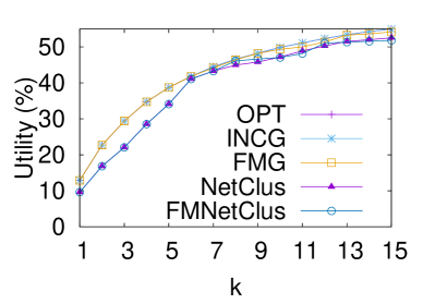
(a) Utility.

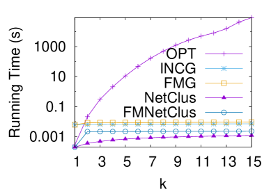
(b) Running time.

Figure 4: Comparison with optimal at $\tau=0.8$ Km.

Since this integer linear program based optimal algorithm requires impractical running times, we ran it only on the Beijing-Small dataset mainly to assess the quality of the other algorithms. Fig. 4 shows that the average utility of all the algorithms are quite close to Opt although the running times are much better. (Note that the utilities in these and all subsequent figures are plotted as a percentage of the total number of trajectories.) Opt requires hours to complete even for this small dataset and, therefore, is not practical at all. Consequently, we did not experiment with Opt any further.

8.4 Quality Results

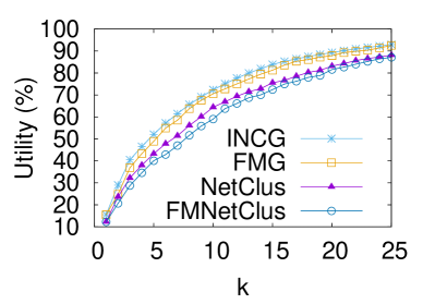
(a) Varying $k$

(b) Varying $\tau$

Figure 5: Quality results.

Fig. 5 shows the utility yields for different values of $k$ and $\tau$. The utilities of NetClus are close to that of IncG and are within 93% of it on an average. Owing to high memory requirements (for reasons to be discussed in the next section), IncG and FMG could not run beyond $\tau=1.2$ Km. The utilities of FMG and FMNetClus are very close to that of IncG and NetClus, respectively.

8.5 Memory Footprint

$\tau$ (in Km.)	IncG	FMG	NetClus	FMNetClus
0.1	7.04	7.90	6.43	7.09
0.2	9.14	10.00	4.17	4.81
0.4	13.47	14.34	3.67	3.94
0.8	19.58	20.44	3.22	3.64
1.2	23.98	24.85	3.52	3.88
1.6	Out of memory		3.41	3.98

Table 9: Memory footprint of different algorithms (in GB).

Table 9 shows that the memory footprints of NetClus and FMNetClus are significantly less than those of IncG and FMG. As the coverage threshold $\tau$ increases, the size of the covering sets, $TC$ and $SC$, used in IncG and FMG, increase sharply. Consequently, these algorithms could not scale beyond $\tau=1.2$ Km. On the other hand, with higher $\tau$, NetClus and FMNetClus use lower resolution clustering instances leading to higher data compression, thereby resulting in lower memory footprints. The FM sketch based schemes require slightly more memory than their counterparts, due to storage of multiple bit vectors for each site or cluster, as applicable.

8.6 Performance Results

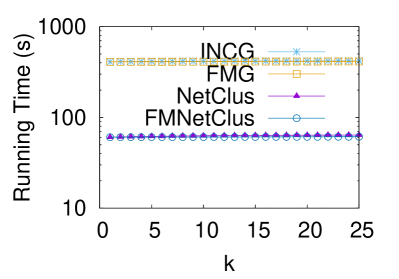
(a) Varying $k$

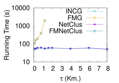
(b) Varying $\tau$

Figure 6: Running time performance.

We next measure the performance of the algorithms for different values of $k$ and $\tau$. Fig. 6 shows that for $\tau\leq 1.2$ km., NetClus and FMNetClus are up to $36$ times faster than IncG and FMG, respectively. For $\tau>1.2$ km., as stated in the previous section, IncG and FMG fail to run due to high memory overheads. When $\tau$ increases, NetClus (and FMNetClus) uses a higher index instance having lesser number of clusters, leading to its efficiency. On the other hand, IncG and FMG use $TC$ and $SC$ covering sets of increasingly larger size, resulting in poor performance.

Note that the plots in Fig. 6a appear to be linear w.r.t. $k$. This is because (i) the initial cost of computing the covering sets significantly dominates the iterative phase of the algorithms, (ii) the running times are plotted in log-scale.

Although FMNetClus (FMG) offers a speed up of about $5$ times in the algorithm running time when compared to NetClus (IncG respectively), its effect is negated by a relatively large initial pre-processing time required for computing the covering sets. Due to this fact, we only compare the results of NetClus with that of IncG in the subsequent sections.

8.7 Extensions and Variants of TOPS

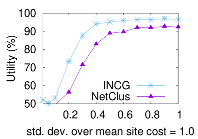
(a) Cost.

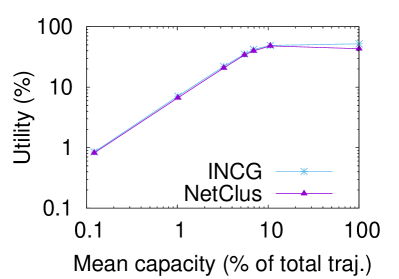
(b) Capacity.

Figure 7: Utilities for TOPS extensions.

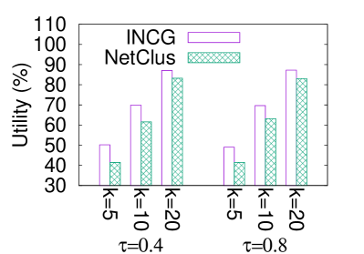
(a) Utility.

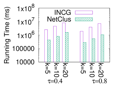
(b) Running time.

Figure 8: Tops2: A variant of TOPS.

We next show results of NetClus on different TOPS extensions and variants (discussed in Sec. 7) over the Beijing dataset.

Tops-Cost: We consider a budget of $B=5.0$ and $\tau=0.8$ Km. The cost of each site was assigned using a normal distribution with mean $\mu=1.0$ and standard deviation varied between $\sigma\in[0,1]$ (the least cost of a site was constrained to be $0.1$). Fig. 7a shows that the utility increases with standard deviation (note that $\sigma=0$ degenerates to basic TOPS). This is due to the fact that with higher standard deviation, more number of sites can be chosen with lower costs which ultimately leads to larger number of trajectories being covered. The increased number of iterations does not increase the running time much since it is a small overhead on the initial costs (Fig. 9).

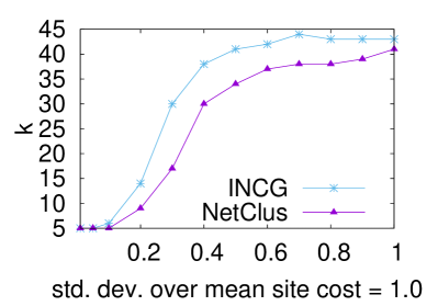
(a) Number of sites.

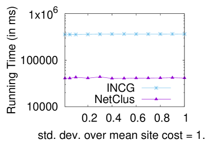
(b) Running time.

Figure 9: TOPS under cost constraint.

Tops-Capacity: We consider $k=5$ and $\tau=0.8$ Km. The sites were assigned varying capacities drawn from a normal distribution where the mean was varied in the range $[0.1\%,100\%]$ of the total number of trajectories, and the standard deviation fixed at $10\%$ of the mean. (note that mean capacity of $100\%$ corresponds to basic unconstrained TOPS). Fig. 7b shows that, as expected, utility increases with mean capacity. NetClus has almost the same utility as that of IncG. We do not show the running time plots, as the algorithms for Tops-Capacity are almost the same as those for TOPS and, hence, exhibit similar performance.

Tops2: Finally, we study the Tops2 variant where the preference function $\psi$ was a convex function of the distance between the site and trajectory. The results, shown in Fig. 8, portray that NetClus has utility close to that of IncG, while being about an order of magnitude faster.

8.8 Updates of Sites and Trajectories

# Trajectories added	Update time	# Candidate sites added	Update time
10000	22.83 s	10000	1.26 s
20000	44.58 s	20000	1.56 s
30000	74.07 s	30000	1.76 s
40000	92.06 s	40000	1.85 s
50000	122.69 s	50000	2.10 s

Table 10: Index update cost.

Table 10 shows that NetClus efficiently processes additions of trajectories and candidate sites over the index structure (Sec. 6). Adding a trajectory requires more time than that for a candidate site since a trajectory passes through multiple clusters in general and the covering sets, etc. of all those clusters need to be updated. Adding a site, on the other hand, requires simply finding the cluster it is in and updating the cluster representative, if applicable.

8.9 Robustness with Parameters

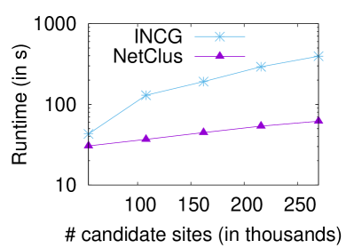
(a) Number of sites.

(b) Number of trajectories.

Figure 10: Scalability results ($k=5$ and $\tau=0.8$ Km).

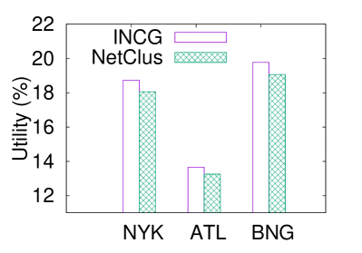
(a) Utility.

(b) Running time.

Figure 11: Effect of city geometries ($k=5$ and $\tau=0.8$ Km).

(a) Utility.

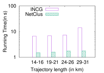
(b) Running time.

Figure 12: Effect of trajectory length ($k=5$ and $\tau=0.8$ Km).

Number of Sites and Trajectories: Fig. 10 shows scalability results with varying number of candidate sites and trajectories on the Beijing dataset. NetClus is about an order of magnitude faster than IncG.

City Geometries: We experimented with three typical city geometries, Atlanta, New York, and Bangalore (Fig. 11). New York has a star topology while Bangalore is poly-centric. Consequently, Bangalore has a larger utility percentage. Since Atlanta has a mesh structure with trajectories distributed all over the city, its utility is lowest. There is not much difference in the running times, though. Bangalore has least running time due to its smaller road network.

Length of Trajectories: To determine the effect of length of trajectories, the trajectories were divided into four classes based on their lengths and from each of the classes, 5,000 trajectories were sampled (Fig. 12). Longer trajectories are easier to cover since they pass through more number of candidate sites over a larger area and, therefore, exhibit higher utility than the shorter ones. The running time also increases with trajectory length due to more number of update operations of the marginal utilities.

8.10 Index Construction

$R_{p}$ (Km)	$\kappa$	$\bar{|\Lambda|}$	$\bar{|\mathcal{TL}|}$	$\bar{|\mathcal{CL}|}$	Run-time (s)
0.0093	258340	1.04	561.88	4.29	269.35
0.0286	195910	1.15	571.41	6.43	239.58
0.0163	233729	1.38	592.45	12.62	255.60
0.0500	153210	1.76	626.18	19.44	221.79
0.0875	112223	2.40	675.60	26.04	204.38
0.1531	76836	3.51	757.03	45.38	192.12
0.2680	48288	5.58	895.19	64.27	188.25
0.4689	28510	9.46	1162.93	53.74	205.74
0.8207	15775	17.10	1525.09	42.73	281.62
1.4361	8258	32.66	2162.01	35.62	537.27
2.5133	4202	64.18	3092.64	21.73	1300.12
4.3982	2024	133.24	4148.03	12.49	3231.92
7.6968	938	287.51	7537.33	3.51	7333.60

Table 11: Details of indexing for Beijing road network comprising of 269,686 nodes with $\gamma=0.75$.

Referring to Table 11, we observe that as the cluster radius $R_{p}$ increases, the number of clusters $\eta_{p}$ decreases as the average dominating set sizes $\bar{|\Lambda|}$ increases. Therefore, the average number of trajectories passing through a cluster $\bar{|\mathcal{TL}|}$ also increases. The average number of neighbors of a cluster $\bar{|\mathcal{CL}|}$ initially increases but finally decreases. Importantly, we observe that the offline index construction times across different cluster radii are practical.

9 Related Work

The related work falls in two main classes, optimal location queries [14, 17, 40, 11, 28], and flow based facility location problems [7, 5, 2, 6, 4, 3].

An optimal location (OL) query has three inputs: a set of facilities, a set of users, and a set of candidate sites. The objective is to determine a candidate site to set up a new facility that optimizes an objective function based on the distances between the facilities and the users. Comparing OL query with TOPS query, we note that: (a) While fixed user locations are considered for OL queries, TOPS uses trajectories of users. (b) OL queries report only a single optimal location, while TOPS reports $k$ locations. (c) Unlike OL queries that are solvable in polynomial time, TOPS is NP-hard (it is polynomially solvable only for $k=1$).

Recently, [28] studied OL queries on trajectories over a road network. Two algorithms were proposed to compute the optimal road segment to host a new service. Their work has quite a few limitations and differences when compared with our work: (a) Since a single optimal road segment is reported, their problem is polynomially solvable. (b) Their work identifies the optimal road segment, rather than the optimal site. (c) There is no analysis on the quality of the reported optimal road segment, either theoretically or empirically. (d) It is not shown how does the reported road segment performs for other established metrics, such as number of new users covered, distance traveled by the users to avail the service, etc.

Facility location problems [13, 18] typically consider a set of users, and a set of candidate sites. The goal is to identify a set of $k$ candidate sites that optimize certain metrics such as covering maximum number of users, or minimizing the average distance between a user and its nearest facility, etc. Almost all of these problems are NP-hard. While early works assumed that the users are static, mobile users are now considered. The flow based facility location works [7, 5, 2, 6, 4, 3] assume a flow model to characterize human mobility, instead of using real trajectories. A fairly comprehensive literature survey is available in [8]. We briefly outline the major works related to the different versions of TOPS queries that have been discussed in Sec. 7. In [7], few exact and approximate algorithms for Tops1 and Tops4, were presented, under the restriction that a customer would stay on the path, i.e., $\tau=0$. Later, in [2], few generalizations of the model were proposed, where the customers were allowed to deviate. These include Tops1, Tops2 and Tops3 problems. Further generalizations of Tops1 were examined in [6], with probabilistic customer flows, single and multiple flow interceptions, and fixed and variable installation costs of the services. Several existing flow-based facility location models were generalized in [43]. Few flow refueling location models have been proposed in [31, 26, 34] for sitingalternative- fuel stations. We have already discussed how our work differs from these works in Sec. 1.

Recently, a greedy heuristic was proposed for the Tops1 problem in [29]. under the assumption that $\tau=0$, i.e., no customer deviations are allowed. We present a detailed study of the Tops1 problem in [36], with arbitrary value of $\tau$.

10 Conclusions

In this paper, we have proposed a generic TOPS framework to solve the problem of finding facility locations for trajectory-aware services. We showed that the problem is NP-hard, and proposed a greedy heuristic with constant factor approximation bound. However, this heuristic does not scale for large datasets. Thus, we developed an index structure, NetClus, to make it practical for city-scale road networks. Extensive experiments over real datasets showed that NetClus yields solutions that are comparable with those of the greedy heuristic, while being significantly faster, and low in memory overhead. The proposed framework can handle a wide class of objectives, and additional constraints, thus making it highly generic and practical.

Appendix A Algorithms for TOPS

A.1 Linearization for Optimal Algorithm

Each inequality in Ineq. (6) can be expressed as

$$U_{j}\leq\max\{U_{j1},U_{j2}\}$$

where

$$U_{j1}\leq\max\{\psi(T_{j},s_{i})x_{i}|1\leq i\leq\lfloor n/2\rfloor\}$$

and

$$U_{j2}\leq\max\{\psi(T_{j},s_{i}).x_{i}|\lfloor n/2\rfloor+1\leq i\leq n\}$$

The terms $U_{j1}$ and $U_{j2}$ can be recursively expressed in the same manner as in case of $U_{j}$.

Finally, the constraint $U_{j}\leq\max\{U_{j1},U_{j2}\}$ can be linearized as follows:

$$U_{j1} \leq U_{j2}+M.y_{j}$$

$$U_{j2} \leq U_{j1}+M.(1-y_{j})$$

$$U_{j} \leq U_{j2}+M.y_{j}$$

$$U_{j} \leq U_{j1}+M.(1-y_{j})$$

$$y_{j} \in\{0,1\}$$

where $M$ is a sufficiently large number.

A.2 Inc-Greedy Algorithm

Algorithm 1 Inc-Greedy

1:procedure Inc-Greedy($k,\tau,\psi$)

2:    Compute the sets $TC,SC$ and the site-weights.

3:    $\mathcal{Q}_{0}\leftarrow\varnothing$

4:    for each $s_{i}\in\mathcal{S}$ do

5:       $U_{0}(s_{i})\leftarrow w_{i}$

6:       $\forall T_{j}\in TC(s_{i}),\alpha_{ji}\leftarrow\psi(T_{j},s_{i})$     

7:    $\forall T_{j}\in\mathcal{T},U_{j}\leftarrow 0$

8:    for each $\theta=1,\dots,k$ do

9:       $s_{\theta}\leftarrow\arg\max_{\forall s_{i}\in\mathcal{S}\setminus\mathcal{Q}_{\theta-1}}\{U(\mathcal{Q}_{\theta-1}\cup\{s_{i}\})-U(\mathcal{Q}_{\theta-1})\}$

10:       $\mathcal{Q}_{\theta}\leftarrow\mathcal{Q}_{\theta-1}\cup\{s_{\theta}\}$

11:       for each trajectory $T_{j}\in TC(s_{\theta})$ do

12:          $U_{j}\leftarrow\max(U_{j},\psi(T_{j},s_{\theta}))$

13:          if $U_{j}$ changes then

14:             for each site $s_{i}\in SC(T_{j}),s_{i}\notin\mathcal{Q}_{\theta}$ do

15:                $\alpha_{ji}^{\prime}\leftarrow\max(0,\psi(T_{j},s_{i})-U_{j})$

16:                $U_{\theta}(s_{i})\leftarrow U_{\theta-1}(s_{i})-(\alpha_{ji}-\alpha_{ji}^{\prime})$

17:                $\alpha_{ji}\leftarrow\alpha_{ji}^{\prime}$                                   

The Inc-Greedy procedure is outlined in Algorithm 1. The algorithm begins by computing the sets $TC,SC$, and the site-weights. It then initializes the marginal utilities of each site $s_{i}\in\mathcal{S}$ to its site weight, i.e., $U_{0}(s_{i})=w_{i}$. Further, for each trajectory $T_{j}\in TC(s_{i})$, it initializes $\alpha_{ji}=\psi(T_{j},s_{i})$.

In iteration $\theta=1,\dots,k$, it selects the site $s_{\theta}$ with maximal marginal utility, i.e., $\forall s_{i}\notin\mathcal{Q}_{\theta-1},U_{\theta}(s_{\theta})\geq U_{\theta}(s_{i})$. If multiple candidate sites yield the same maximal marginal gain we choose the one with maximal weight. Still, if there are ties, then without loss of generality, the site with the highest index is selected.

For each trajectory $T_{j}\in TC(s_{\theta})$ (line 11), first the utility $U_{j}$ is updated (line 12). In case there is a gain in $U_{j}$, each site $s_{i}\in SC(T_{j})$ is processed as indicated in line 14. In line 15, the new marginal utility of trajectory $T_{j}$ w.r.t. site $s_{i}$ is computed. Using this value, the marginal utility of site $s_{i}$ and $\alpha_{ji}$ are updated.

Appendix B NetClus

B.1 Clustering based on Jaccard Similarity

$\tau$ (Km)	Running Time (s)	Memory (in GB)
0	2890	3.88
0.2	12473	8.93
0.4	26693	9.98
0.8	28391	14.23
1.2	29058	16.57
1.6	32647	20.85
2.0	34618	26.74
2.4	Out of memory

Table 12: Performance of Jaccard similarity based clustering for Beijing road network using a Jaccard distance threshold $\alpha=0.8$.

Given two nodes $s_{i},s_{j}\in\mathcal{S}$, the Jaccard similarity between their trajectory covers is

$$J_{s}(s_{i},s_{j}) =\frac{|TC(s_{i})\cap TC(s_{j})|}{|TC(s_{i})\cup TC(s_{j})|}$$

The Jaccard distance is

$$J_{d}(s_{i},s_{j})=1-J_{s}(s_{i},s_{j})$$

The nodes in the road network $V$ are clustered using the above measure as follows.

The node $v_{1}$ with the highest weight, i.e., the one whose sum of preference scores over the covered trajectories as defined in Sec. 3.2, is chosen as the first cluster center of the cluster $g_{1}$. All nodes that are within a threshold of $\alpha$ Jaccard distance from $v_{1}$ are added to $g_{1}$. From the remaining set of unclustered nodes, the node with the highest weight is chosen as a cluster center, and the process is repeated until each node is clustered.

The results of clustering on the Beijing dataset are shown in Table 12. The limitations of Jaccard similarity based clustering are explained in Sec. 4.

B.2 Complexity Analysis of Greedy-GDSP

Theorem 18.

Greedy-GDSP runs in $O(|V|.(\nu\log\nu+\eta))$ time where $\nu$ is the maximum number of vertices that are reachable within the largest round-trip distance $R_{max}$ from any vertex $v$, and $\eta$ is the number of clusters returned by the algorithm.

Proof B.1.

As the underlying graph models a road network which is roughly planar, we assume that the number of edges (i.e., road segments) incident on any set of $\nu$ vertices is $O(\nu)$. Since the cost of running the shortest path algorithm from a given node in a graph $G=(V,E)$ is $O(|E|\log|V|)$ [12], therefore, the initial distance computation for a given source vertex requires $O(\nu\log\nu)$ time. Thus, the distance computation across all the vertices in $V$ takes $O(|V|.\nu\log\nu)$. The neighbors of each node $v$ can be maintained as a list sorted by the round-trip distance from $v$. Therefore, computing the dominating set for a particular $R$ requires at most $\nu$ time for each vertex. The total time for the construction of dominating sets, hence, is $O(|V|.\nu)$.

Choosing the vertex with the largest incremental dominating set requires bitwise OR operations of FM sketches. For $|V|$ vertices, there are at most $|V|-1$ such operations, each requiring $O(f)$ time (since there are $f$ copies of FM sketches each with a constant size of $32$ bits). As the number of clusters produced is $\eta$, the running time is $O(|V|.\eta)$.

The total running time is, therefore, $O(|V|.(\nu\log\nu+\eta))$.

B.3 Complexity of NetClus

Theorem 19.

The time and space complexities of NetClus are $O(k.\eta_{p}.\xi_{p})$ and $O(\sum_{p=1}^{t}(\eta_{p}(\xi_{p}+\lambda_{p})))$ respectively.

Proof B.2.

The number of cluster representatives, $|\widehat{\mathcal{S}}|$ is at most the number of clusters, $\eta_{p}$. For any cluster $g_{i}\in p$, $|\mathcal{TL}(g_{i})|=O(\xi_{p})$. We assume that the number of neighboring clusters for any cluster is bounded by a constant, i.e., $|\mathcal{CL}(g_{i})|=O(1)$. (Table 11 that lists typical mean values of $|\mathcal{CL}(g_{i})|$ empirically supports the assumption.) Hence, computing the set $\widehat{TC}(r_{i})$ requires at most $O(\xi_{p})$ time. The total time across all the $\eta_{p}$ clusters, therefore, is $O(\eta_{p}.\xi_{p})$. The inverse maps $\widehat{CC}(T_{j})$ for the trajectories can be computed along with $\widehat{TC}(r_{i})$. Hence, the total time remains $O(\eta_{p}.\xi_{p})$. Using Th. 7, the subsequent Inc-Greedy phase requires $O(k.\eta_{p}.\xi_{p})$ time. Therefore, the overall time complexity of the algorithm is $O(k.\eta_{p}.\xi_{p})$.

We next analyze the space complexity for a particular index instance $p$. Storing the sets $\mathcal{TL}(g_{i})$, each of size at most $\xi_{p}$, across all the $\eta_{p}$ clusters require $O(\eta_{p}.\xi_{p})$ space. Storing the inverse maps $CC(T_{j})$ for all the trajectories, thus, also requires $O(\eta_{p}.\xi_{p})$ space. As there are at most $\lambda_{p}$ vertices in any cluster, storing their ids and distances from the cluster center requires $O(\lambda_{p})$ space for each cluster. Assuming $|\mathcal{CL}(g_{i})|=O(1)$, the total storage cost for a cluster is $O(\lambda_{p})$. Therefore, the total storage cost is $O(\eta_{p}.(\xi_{p}+\lambda_{p}))$. Summing across all the index instances, the entire space complexity is $O(\sum_{p=1}^{t}(\eta_{p}(\xi_{p}+\lambda_{p})))$.

References

- [1] P. Banerjee, S. Ranu, and S. Raghavan. Inferring uncertain trajectories from partial observations. In ICDM, pages 30–39, 2014.
- [2] O. Berman, D. Bertsimas, and R. C. Larson. Locating discretionary service facilities, ii: maximizing market size, minimizing inconvenience. Operations Research, 43(4):623–632, 1995.
- [3] O. Berman and D. Krass. Flow intercepting spatial interaction model: a new approach to optimal location of competitive facilities. Location Science, 6(1):41–65, 1998.
- [4] O. Berman and D. Krass. The generalized maximal covering location problem. Computers & Operations Research, 29(6):563–581, 2002.
- [5] O. Berman, D. Krass, and C. W. Xu. Locating discretionary service facilities based on probabilistic customer flows. Transportation Science, 29(3):276–290, 1995.
- [6] O. Berman, D. Krass, and C. W. Xu. Locating flow-intercepting facilities: New approaches and results. Annals of Operations research, 60(1):121–143, 1995.
- [7] O. Berman, R. C. Larson, and N. Fouska. Optimal location of discretionary service facilities. Transportation Science, 26(3):201–211, 1992.
- [8] M. Boccia, A. Sforza, and C. Sterle. Flow intercepting facility location: Problems, models and heuristics. J. Mathematical Modelling and Algorithms, 8(1):35–79, 2009.
- [9] L. Chen and R. Ng. On the marriage of edit distance and Lp norms. In VLDB, 2004.
- [10] N. Chen, J. Meng, J. Rong, and H. Zhu. Approximation for dominating set problem with measure functions. Computing and Informatics, 23(1):37–49, 2012.
- [11] Z. Chen, Y. Liu, R. C.-W. Wong, J. Xiong, G. Mai, and C. Long. Efficient algorithms for optimal location queries in road networks. In SIGMOD, pages 123–134, 2014.
- [12] T. H. Cormen, C. E. Leiserson, R. L. Rivest, and C. Stein. Introduction to Algorithms. MIT Press, 2009.
- [13] Z. Drezner. Facility location: a survey of applications and methods. Springer, 1995.
- [14] Y. Du, D. Zhang, and T. Xia. The optimal-location query. In Advances in Spatial and Temporal Databases, pages 163–180, 2005.
- [15] P. Flajolet and G. N. Martin. Probabilistic counting algorithms for data base applications. J. Computer and System Sciences, 31(2):182–209, 1985.
- [16] E. Frentzos, K. Gratsias, and Y. Theodoridis. Index-based Most Similar Trajectory Search. In ICDE, pages 816–825, 2007.
- [17] P. Ghaemi, K. Shahabi, J. P. Wilson, and F. Banaei-Kashani. Optimal network location queries. In SIGSPATIAL GIS, pages 478–481, 2010.
- [18] H. W. Hamacher and Z. Drezner. Facility location: applications and theory. Springer, 2002.
- [19] T. W. Haynes, S. Hedetniemi, and P. Slater. Fundamentals of Domination in Graphs. CRC Press, 1998.
- [20] W. He, D. Li, T. Zhang, L. An, M. Guo, and G. Chen. Mining regular routes from gps data for ridesharing recommendations. In SIGKDD, pages 79–86, 2012.
- [21] H. Jeung, M. L. Yiu, X. Zhou, C. S. Jensen, and H. T. Shen. Discovery of convoys in trajectory databases. Proceedings of the VLDB Endowment, 1(1):1068–1080, 2008.
- [22] P. Kalnis, N. Mamoulis, and S. Bakiras. On discovering moving clusters in spatio-temporal data. In International Symposium on Spatial and Temporal Databases, pages 364–381. Springer, 2005.
- [23] B. kee Yi, H. V. Jagadish, and C. Faloutsos. Efficient Retrieval of Similar Time Sequences Under Time Warping. In ICDE, 1998.
- [24] S. Khuller, A. Moss, and J. S. Naor. The budgeted maximum coverage problem. Information Processing Letters, 70(1):39–45, 1999.
- [25] V. Kolar, S. Ranu, A. P. Subramanian, Y. Shrinivasan, A. Telang, R. Kokku, and S. Raghavan. People in motion: Spatio-temporal analytics on call detail records. In COMSNETS, pages 1–4, 2014.
- [26] M. Kuby, L. Lines, R. Schultz, Z. Xie, J.-G. Kim, and S. Lim. Optimization of hydrogen stations in florida using the flow-refueling location model. International journal of hydrogen energy, 34(15):6045–6064, 2009.
- [27] J.-G. Lee, J. Han, and K.-Y. Whang. Trajectory clustering: a partition-and-group framework. In Proceedings of the 2007 ACM SIGMOD international conference on Management of data, pages 593–604. ACM, 2007.
- [28] X. Li, V. Čeikute, C. S. Jensen, and K.-L. Tan. Trajectory based optimal segment computation in road network databases. In SIGSPATIAL GIS, pages 396–399, 2013.
- [29] Y. Li, J. Bao, Y. Li, Y. Wu, Z. Gong, and Y. Zheng. Mining the most influential k-location set from massive trajectories. In Proceedings of the 24th ACM SIGSPATIAL International Conference on Advances in Geographic Information Systems, page 51. ACM, 2016.
- [30] Z. Li, B. Ding, J. Han, and R. Kays. Swarm: Mining relaxed temporal moving object clusters. Proceedings of the VLDB Endowment, 3(1-2):723–734, 2010.
- [31] S. Lim and M. Kuby. Heuristic algorithms for siting alternative-fuel stations using the flow-refueling location model. European Journal of Operational Research, 204(1):51–61, 2010.
- [32] X. Lin, Y. Yuan, Q. Zhang, and Y. Zhang. Selecting stars: The k most representative skyline operator. In ICDE, pages 86–95, 2007.
- [33] Y. Lou, C. Zhang, Y. Zheng, X. Xie, W. Wang, and Y. Huang. Map-matching for low-sampling-rate gps trajectories. In GIS, pages 352–361, 2009.
- [34] S. MirHassani and R. Ebrazi. A flexible reformulation of the refueling station location problem. Transportation Science, 47(4):617–628, 2012.
- [35] S. Mitra, S. Ranu, V. Kolar, A. Telang, A. Bhattacharya, R. Kokku, and S. Raghavan. Trajectory aware macro-cell planning for mobile users. In INFOCOM, 2015.
- [36] S. Mitra, P. Saraf, R. Sharma, A. Bhattacharya, S. Ranu, and H. Bhandari. NetClus: A scalable framework for locating top-k sites for placement of trajectory-aware services. ICDE, 2017.
- [37] G. L. Nemhauser, L. A. Wolsey, and M. L. Fisher. An analysis of approximations for maximizing submodular set functions. Mathematical Programming, 14(1):265–294, 1978.
- [38] S. Ranu, P. Deepak, A. D. Telang, P. Deshpande, and S. Raghavan. Indexing and matching trajectories under inconsistent sampling rates. In ICDE, 2015.
- [39] M. Vlachos, D. Gunopoulos, and G. Kollios. Discovering similar multidimensional trajectories. In ICDE, 2002.
- [40] X. Xiao, B. Yao, and F. Li. Optimal location queries in road network databases. In ICDE, pages 804–815, 2011.
- [41] J. Yuan, Y. Zheng, X. Xie, and G. Sun. Driving with knowledge from the physical world. In KDD, pages 316–324, 2011.
- [42] J. Yuan, Y. Zheng, C. Zhang, W. Xie, X. Xie, G. Sun, and Y. Huang. T-drive: driving directions based on taxi trajectories. In SIGSPATIAL GIS, pages 99–108, 2010.
- [43] W. Zeng, I. Castillo, and M. J. Hodgson. A generalized model for locating facilities on a network with flow-based demand. Networks and Spatial Economics, 10(4):579–611, 2010.
- [44] W. Zeng, M. J. Hodgson, and I. Castillo. The pickup problem: consumers’ locational preferences in flow interception. Geographical Analysis, 41(1):107–126, 2009.
- [45] D. Zhang, Y. Du, T. Xia, and Y. Tao. Progressive computation of the min-dist optimal-location query. In Proceedings of the 32nd international conference on Very large data bases, pages 643–654. VLDB Endowment, 2006.