Practical Weak Lensing Shear Measurement with Metacalibration

Abstract

Metacalibration is a recently introduced method to accurately measure weak gravitational lensing shear using only the available imaging data, without need for prior information about galaxy properties or calibration from simulations. The method involves distorting the image with a small known shear, and calculating the response of a shear estimator to that applied shear. The method was shown to be accurate in moderate sized simulations with galaxy images that had relatively high signal-to-noise ratios, and without significant selection effects. In this work we introduce a formalism to correct for both shear response and selection biases. We also observe that, for images with relatively low signal-to-noise ratios, the correlated noise that arises during the metacalibration process results in significant bias, for which we develop a simple empirical correction. To test this formalism, we created large image simulations based on both parametric models and real galaxy images, including tests with realistic point-spread functions. We varied the point-spread function ellipticity at the five percent level. In each simulation we applied a small, few percent shear to the galaxy images. We introduced additional challenges that arise in real data, such as detection thresholds, stellar contamination, and missing data. We applied cuts on the measured galaxy properties to induce significant selection effects. Using our formalism, we recovered the input shear with an accuracy better than a part in a thousand in all cases.

1. Introduction

Weak gravitational lensing is a fascinating phenomenon that has become a useful tool for testing our theories of gravity, measuring the properties and distribution of dark matter, and characterizing the accelerated expansion of the universe known as dark energy (for a review, see Hoekstra & Jain, 2008).

Light passing massive objects undergoes a deflection, and the amount of this deflection depends on all the mass in the “lens”, both luminous and dark. The deflection distorts, or “shears”, the observed shape of extended objects such as galaxies, and this shear is spatially correlated. By studying these spatial correlations, one can infer the correlations in the mass that caused the lensing. One can study these correlations at any place in the universe, including the locations of galaxies (Mandelbaum et al., 2006), clusters of galaxies (Johnston et al., 2007), voids (Melchior et al., 2014), and even correlations without reference to any particular lensing objects (Kilbinger et al., 2013). Because the effect depends on the geometry of the lens-source system as well as mass, the expansion history and growth of structure can be inferred, and thus weak lensing is also sensitive to dark energy (Heymans et al., 2013).

Pioneered as a measurement technique in the 1980s and 1990s, weak lensing was quickly recognized to be complimentary to more standard dynamical techniques (Tyson et al., 1984). Because the effect is independent of the dynamical state of the lensing mass, it can be used to study the distribution of mass in systems that are far from equilibrium (Clowe et al., 2006). And because the effect can be measured nearly anywhere, it can be used to probe very large scales, measuring the correlation between objects and large scale structure (Sheldon et al., 2009).

Thus far, progress in measurement has been limited by technical challenges, a few of which we will outline below. To set a scale of reference, the weak lensing shear due to a foreground lens typically introduces correlations in the shapes of background galaxies at the percent level. We would like to measure this percent level signal to approximately a part in a thousand in upcoming imaging surveys (Huterer et al., 2006).

There have traditionally been two approaches to measuring shear from galaxy images: measuring moments of the light distribution and fitting models.

In the model fitting approach, a parametric model is convolved by an estimate of the point-spread function (PSF) of the atmosphere and instrument, and fit to the galaxy surface brightness profile. The shear estimator, the “shape” of the galaxy, is then determined from the parameters of this model. This method is limited for two primary reasons: first, in order for the shear inference to be accurate, the model must accurately reproduce the galaxy profile before noise and convolution by the PSF, which requires a large number of parameters. If the model cannot sufficiently reproduce the galaxy the estimator is said to exhibit “model bias” (Bernstein, 2010). The second is the bias in the nonlinear model fitting caused by noise, which is significant for images with low signal-to-noise ratios ($S/N$), and is difficult to predict (Hirata et al., 2004; Refregier et al., 2012; Melchior & Viola, 2012). This “noise bias” is made worse if large number of model parameters are used in an attempt to accurately represent the galaxy.

Because of these biases, model fitting methods require additional calibration. However, there are no absolute calibration sources in the universe that can be used to derive a calibration. Instead, image simulations have often been used to determine the shear calibration (e.g. Zuntz et al., 2013; Miller et al., 2013; Fenech Conti et al., 2017; Refregier & Amara, 2014; Jee et al., 2016). These simulations must include all the relevant details of the real universe in order to provide an accurate calibration. It has been suggested that model biases can partly be alleviated without image simulations if a sufficiently flexible statistical framework is used (Schneider et al., 2015), but this has not yet been demonstrated.

Another traditional shear measurement technique uses the second moments of the galaxy light distribution, after correction for the effect of the PSF (e.g. Kaiser et al., 1995; Bernstein, 2010). These methods can be made quite accurate for galaxy images with high $S/N$, with little model bias (Bernstein, 2010; Okura & Futamase, 2016). However, unlike model fitting approaches, missing data and light from nearby objects cannot be “masked-out” or ignored. Also, these methods still suffer the “noise bias” found in model fitting methods as a result of the nonlinear fitting involved with the measurement. Without further development, these methods are not accurate at the part-in-a-thousand level.

Finally, selection effects can bias the recovered shear in both model fitting and moment based methods, but the corrections are typically considered as separate from the shear estimation, to be inferred as part of a calibration based on simulations (Jarvis et al., 2016; Fenech Conti et al., 2017)).

Methods have recently been developed to avoid some of these biases without relying on calibration from simulations. The method of Zhang et al. (2017) involves measuring the weighted moments in Fourier space, after subtracting an appropriate noise power spectrum to deal with noise effects, and deconvolving the PSF. No nonlinear fitting is performed. The shear is then estimated either from the ratio of sums of these moments (Zhang et al., 2015), or the PDF of the un-normalized moments is symmetrized in order to infer an applied shear (Zhang et al., 2017). The sum method was shown to be accurate at the part-in-a-thousand level in challenging simulations, but with unacceptably high noise. The PDF symmetrization method was shown to be more precise, but the simulations used were not large enough to determine the accuracy of the method to the part-in-a-thousand level. No formalism has been proposed as yet to deal with selection effects.

Another new approach is the Bayesian Fourier Domain (BFD) method for shear inference introduced by Bernstein & Armstrong (2014) and further developed by Bernstein et al. (2016). A rigorous Bayesian framework was presented, in which prior information on galaxy images from much deeper data is included. Un-normalized moments in Fourier space are used as the basic data vector, avoiding nonlinear fitting issues. BFD is also the first method for which selection effects are corrected for naturally in the formalism, without use of external simulations. The method was tested in Bernstein et al. (2016) using a challenging simulation. In that initial study, a bias of $\sim 2\times 10^{-3}$ was detected, falling just short of the part-in-a-thousand target. However, given its rigorous foundation, it seems possible that the desired accuracy will be achieved with further technical development. The required prior information from deep data should in principle be available to current and future surveys (The Dark Energy Survey Collaboration, 2005; Takada, 2010; Ivezic et al., 2008; Laureijs et al., 2011; Spergel et al., 2015).

Metacalibration (Huff & Mandelbaum, 2017), the subject of this work, is a new method designed to calibrate standard shear estimators, without requiring significant prior information about galaxy properties. This is accomplished by introducing an artificial shear to images, and calculating how the shear estimator responds to the applied shear, addressing both model bias and noise bias. Metacalibration can in principle be used to calibrate any shear estimator, including shapes derived from model fitting or weighted moments.

The metacalibration approach is not entirely new. A quite similar idea to metacalibration was introduced by Kaiser (2000), although the full equivalent of metacalibration was not implemented therein. Kaiser et al. (1995) also introduced the use of sheared high-resolution space-based images as a way to provide an overall calibration for a shear estimator.

The metacalibration technique was shown to be accurate in controlled simulations (Huff & Mandelbaum, 2017). However, the simulations used in that study (based on those used in Mandelbaum et al., 2014) contained galaxy images with fairly high $S/N$, and the galaxies were relatively large compared to the PSF size. In a real survey, the images are dominated by small faint galaxies, many of which cannot be reliably detected or measured. Furthermore, owing to the limited number of galaxies in those simulations, the accuracy of the method could only be tested to about three parts in a thousand. In this work we use a more challenging set of simulations.

We will also address other difficulties that arise in real data. During estimation of a shear statistic, further selection beyond a simple detection threshold is often required, such as cutting or binning based on galaxy properties, which can cause significant selection biases. We introduce a formalism to deal with selection effects, for example, cuts on $S/N$ and galaxy size, that are required for any practical analysis.

In real images, stars cannot be perfectly removed from the sample of objects used to measure shear. We will show that metacalibration is robust to the presence of stars in the sample if the PSF is well determined.

Finally, the metacalibration procedure itself correlates the noise across the image, which becomes a dominant source of error for galaxy images with low $S/N$. We introduce a simple image-level correction for this correlated noise.

We show that, in all scenarios we tested, metacalibration is indeed accurate to a part in a thousand.

2. Introduction to Metacalibration

In this section we introduce the basic concepts of metacalibration. We derive the full formalism for shear measurements in §3.

Suppose we have a noisy measurement $e$ that we wish to use for shear estimation. $e$ may be some estimate of an objects two-component ellipticity such that $\mbox{\boldmath$e$}=(e_{1},e_{2})$. We can expand this observable in a Taylor series about zero shear

$$e =\mbox{\boldmath$e$}|_{\gamma=0}+\frac{\partial\mbox{\boldmath$e$}}{\partial\mbox{\boldmath$\gamma$}}\bigg{|}_{\gamma=0}\mbox{\boldmath$\gamma$}+...$$

$$\equiv\mbox{\boldmath$e$}|_{\gamma=0}+\mbox{\mbox{\boldmath$R$}}\mbox{\boldmath$\gamma$}+...$$ (1)

where we have defined the shear response:

$$R \equiv\frac{\partial\mbox{\boldmath$e$}}{\partial\mbox{\boldmath$\gamma$}}\bigg{|}_{\gamma=0}.$$ (2)

Note that the derivative is also with respect to the two-component shear $\gamma$, making $R$ a $2\times 2$ matrix:

$$\mbox{\mbox{\boldmath$R$}}=\left(\begin{array}[]{cc}\partial e_{1}/\partial\gamma_{1}&\partial e_{2}/\partial\gamma_{1}\\ \partial e_{1}/\partial\gamma_{2}&\partial e_{2}/\partial\gamma_{2}\end{array}\right).$$

We can use the ensemble mean of such measurements $e$, for example, measured from a population of galaxies, as a shear estimator. Assuming the shear is small, we can drop terms of order $\gamma^{2}$ and higher (we explore this approximation in §9), such that

$$\langle\mbox{\boldmath$e$}\rangle =\langle\mbox{\boldmath$e$}\rangle|_{\gamma=0}+\langle\mbox{\mbox{\boldmath$R$}}\mbox{\boldmath$\gamma$}\rangle+...$$

$$\approx\langle\mbox{\mbox{\boldmath$R$}}\mbox{\boldmath$\gamma$}\rangle,$$ (3)

where we have also assumed the intrinsic ellipticities of galaxies are randomly oriented such that $\langle\mbox{\boldmath$e$}\rangle|_{\gamma=0}\sim(0,0)$. If we have estimates of $R$ for each galaxy, we can form a weighted average:

$$\langle\mbox{\boldmath$\gamma$}\rangle \approx\langle\mbox{\mbox{\boldmath$R$}}\rangle^{-1}\langle\mbox{\boldmath$e$}\rangle\approx\langle\mbox{\mbox{\boldmath$R$}}\rangle^{-1}\langle\mbox{\boldmath$R$}\mbox{\boldmath$\gamma$}\rangle.$$ (4)

Note the special case of constant shear, where $\gamma$ factors out of the right-hand side.

If the estimator $e$ is unbiased, the mean response matrix $\langle R\rangle$ will be consistent with the identity matrix. If $e$ is a biased estimator, $\langle R\rangle$ will deviate from the identity matrix, and could have significant structure.

The essence of metacalibration (Huff & Mandelbaum, 2017) is to estimate the shear response $R$ for a measurement $e$ directly from image data. The measurement of the shear estimator $e$ is repeated on sheared versions of the galaxy image and these are used to form a finite-difference central derivative. For component $i,j$ we can write

$$R_{i,j}=\frac{e_{i}^{+}-e_{i}^{-}}{\Delta\gamma_{j}},$$ (5)

where $e^{+}$ is the measurement made on an image sheared by $+\gamma$, $e^{-}$ is the measurement made on an image sheared by $-\gamma$, and $\Delta\gamma=2\gamma$.

The shearing is accomplished via a series of image manipulations. The original image $I$ is deconvolved from the point spread function (PSF), sheared, and reconvolved by the another function to suppress the amplified noise that is due to deconvolution. This function should be slightly larger than the original PSF in order to suppress Fourier modes exposed by the shearing that were previously hidden in the finite resolution of the original image. We can represent the series of operations clearly in Fourier space, where convolutions are products and deconvolutions are divisions:

$$\mbox{$\widetilde{I}$}(\gamma)=\left[\left(\mbox{$\widetilde{I}$}/\mbox{$\widetilde{P}$}\right)\oplus\gamma\right]\times\mbox{$\widetilde{P_{d}}$}$$ (6)

where $\widetilde{I}$ and $\widetilde{P}$ are the Fourier transforms of the image and PSF. $\widetilde{P_{d}}$ is the Fourier transform of the function with which the image is reconvolved; we use the subscript $d$ to indicated that the function is “dilated” with respect to the original PSF. Shearing is represented by $\oplus$.

Note that for measurement of the shear estimator $e$, one should use an image passed through these same image manipulations, but without any shear applied. This ensures that the same reconvolution function is used for the shear estimator and the response measurements.

We find that the results are rather insensitive to the choice of applied shear. We tested values in the range of 0.001 to 0.05 and did not see significant changes in the results. We take $\gamma=0.01$.

In practice, the response matrices measured from each image can have significant structure, but the average $\langle R\rangle$ is to good approximation diagonal. Thus, for a straight mean shear measurement the correction in equation 4 reduces to element-wise division. However, measurements such as tangential shear or pairwise two-point functions involve projecting the ellipticities into different coordinate systems. The measurement may require projection of the response matrix as well, which could require using the full response matrix.

One might expect the response to be proportional to the identity matrix if there is no preferred direction in the measurement process. In the simulation tests we present in §6, we found that the diagonal elements can differ by as much as a few parts in a thousand due to the use of a strong PSF anisotropy oriented along the diagonal of the image.

As mentioned, the estimator $e$ can be noisy, but in principle, when averaging over a large ensemble of measurements, the noise does not cause any bias because $\langle R\rangle$ is very well determined (see §2.1). However, when working with images, the metacalibration process itself alters the noise in a coherent way, requiring a correction (see §4.1).

2.1. PSF Anisotropy and Shear Inference

If the PSF correction is not perfect, the leading term $\langle\mbox{\boldmath$e$}\rangle|_{\gamma=0}$ will not be zero. Huff & Mandelbaum (2017) discussed another response, the response of the measurement to the PSF ellipticity, to correct this effect. In this work we instead reconvolve the image by a circular function, which removes most additive effects that are due to the PSF (see §7).

In Huff & Mandelbaum (2017) the simple averaging in equation 4 did not work well because the shape estimators used therein were relatively noisy. Instead, a sophisticated statistical method was developed to infer the shear. For the estimator we use in this work (see §7), the $R$ are relatively well measured, even for galaxies with very low $S/N$, and the average $\langle R\rangle$ is very well determined. We find that using simple averages in equation 4 is adequate to infer the correct shear.

3. Full Metacalibration Formalism

In this section we derive the full metacalibration formalism, including selection effects. First we introduce some notation: in principle, the estimator $e$ can be any set of measurements from an image, but in what follows, without loss of generality, we write the shear estimator $e$ as a two-component ellipticity $\mbox{\boldmath$e$}=(e_{1},e_{2})$. We write the ellipticity measured from a sheared image as $\mbox{\boldmath$e$}^{+}$ and $\mbox{\boldmath$e$}^{-}$, for measurements on positive and negatively sheared images, respectively. We denote the selection probability as $S$; we can also make selections based on sheared parameters, which we denote $S^{+}$ and $S^{-}$, the probability of selection after a positive or negative shear is applied, respectively.

3.1. Response for the Mean Shear

Suppose we wish to use the mean ellipticity as an estimator for the mean shear. The mean ellipticity over a large ensemble can be written as

$$\langle\mbox{\boldmath$e$}\rangle=\int P(\mbox{\boldmath$e$})~{}\mbox{\boldmath$e$}~{}d\mbox{\boldmath$e$},$$ (7)

where $P(\mbox{\boldmath$e$})$ is the probability distribution of $e$. We choose to work with continuous functions so that all derivatives are well defined, in particular the derivative of the selection function that we introduce below.

Assuming each galaxy experiences a small shear and that galaxy orientations are random in the absence of shear, the mean ellipticity can be rewritten, to leading order, as

$$\langle\mbox{\boldmath$e$}\rangle\approx\int d\mbox{\boldmath$e$}\frac{\partial P(\mbox{\boldmath$e$})\mbox{\boldmath$e$}}{\partial\mbox{\boldmath$\gamma$}}\bigg{|}_{\gamma=0}\mbox{\boldmath$\gamma$}~{}d\mbox{\boldmath$e$}=\langle\mbox{\boldmath$R_{\gamma}$}\mbox{\boldmath$\gamma$}\rangle,$$ (8)

where we have ignored the perturbation of the normalization $\int d\mbox{\boldmath$e$}P(\mbox{\boldmath$e$})$ because it leads to terms that are second order or higher in the shear. The mean shear is thus weighted by a response matrix $R_{\gamma}$. This is the same $2\times 2$ response matrix as discussed in §2; we have added the subscript $\gamma$ to differentiate this response from the selection response discussed below. If the $R_{\gamma}$ are known, we can form a weighted-average estimator for the mean shear:

$$\left<\mbox{\boldmath$\gamma$}\right>\approx\mbox{\boldmath$\langle R_{\gamma}\rangle$}^{-1}\left<\mbox{\boldmath$e$}\right>\approx\mbox{\boldmath$\langle R_{\gamma}\rangle$}^{-1}\left<\mbox{\boldmath$R_{\gamma}$}\mbox{\boldmath$\gamma$}\right>.$$ (9)

We can calculate this mean response $\langle R_{\gamma}\rangle$ using quantities measured on artifically sheared images, as discussed in §2. We will approximate the derivatives using finite differences in the shear, such that

$$\langle R_{\gamma}\rangle =\int\frac{\partial P(\mbox{\boldmath$e$})\mbox{\boldmath$e$}}{\partial\mbox{\boldmath$\gamma$}}\bigg{|}_{\gamma=0}d\mbox{\boldmath$e$}\approx\int d\mbox{\boldmath$e$}\left(\frac{P^{+}\mbox{\boldmath$e$}_{i}^{+}-P^{-}\mbox{\boldmath$e$}_{i}^{-}}{\Delta\gamma_{j}}\right)d\mbox{\boldmath$e$}$$

$$=\frac{\langle e_{i}^{+}\rangle-\langle e_{i}^{-}\rangle}{\Delta\gamma_{j}},$$ (10)

where we switched to component notation, such that $i,j$ denotes the derivative of the $i$th ellipticity component with respect to the $j$th shear component. In practice, this averaging is performed over an ensemble of measurements for discrete objects. It is equivalent to averaging the responses as measured for each object.

3.1.1 Selection Effects for the Mean Shear

Now consider a selection that modifies the distribution of the measurement $e$. We will write this selection function as $S(\mbox{\boldmath$e$})$, the probability of selecting an object with ellipticity $e$, although the selection may be indirect, for example, a cut on $S/N$. This selection function could also represent some kind of weighting scheme that indirectly weights by ellipticity.

After introducing a selection, the mean becomes

$$\langle\mbox{\boldmath$e$}\rangle^{S}=\int S(\mbox{\boldmath$e$})~{}P(\mbox{\boldmath$e$})~{}\mbox{\boldmath$e$}~{}d\mbox{\boldmath$e$}.$$ (11)

We will assume the $\int d\mbox{\boldmath$e$}P(\mbox{\boldmath$e$})S(\mbox{\boldmath$e$})=1$, and continue to ignore the higher order effect from changes in the normalization under shear. Again, assuming a small shear and that galaxy orientations are random in the absence of shear, the mean ellipticity after selection can be rewritten, to leading order, as

$$\langle\mbox{\boldmath$e$}\rangle\approx\int d\mbox{\boldmath$e$}\frac{\partial S(\mbox{\boldmath$e$})P(\mbox{\boldmath$e$})\mbox{\boldmath$e$}}{\partial\mbox{\boldmath$\gamma$}}\bigg{|}_{\gamma=0}~{}\mbox{\boldmath$\gamma$}~{}d\mbox{\boldmath$e$}=\langle\mbox{\boldmath$R$}\mbox{\boldmath$\gamma$}\rangle,$$ (12)

Thus, the mean shear in the presence of selections is also weighted by a response term $R$, and this response now includes the shear response as well as the effects of the selections. The probability that an object is selected changes after it is sheared.

This response with selections can be calculated using quantities measured on artifically sheared images. It is useful to examine separately the response of the estimator $e$ to a shear and the response of selection effects to a shear:

$$\langle R\rangle =\int\frac{\partial S(\mbox{\boldmath$e$})P(\mbox{\boldmath$e$})\mbox{\boldmath$e$}}{\partial\mbox{\boldmath$\gamma$}}\bigg{|}_{\gamma=0}d\mbox{\boldmath$e$}$$

$$=\int\left[S(\mbox{\boldmath$e$})\frac{\partial P(\mbox{\boldmath$e$})\mbox{\boldmath$e$}}{\partial\mbox{\boldmath$\gamma$}}\bigg{|}_{\gamma=0}+P(\mbox{\boldmath$e$})\mbox{\boldmath$e$}\frac{\partial S(\mbox{\boldmath$e$})}{\partial\mbox{\boldmath$\gamma$}}\bigg{|}_{\gamma=0}\right]d\mbox{\boldmath$e$}$$ (13)

Note that the first term is identical to the response in equation 8, but now with selections applied. As we show below, the second term represents the response of selection effects to a shear.

We will again approximate the derivatives using finite differences in the shear. Using the notation for measurements on sheared images, introduced in §3, we can rewrite the response as

$$\langle R\rangle \approx\int d\mbox{\boldmath$e$}\left[S\left(\frac{P^{+}e_{i}^{+}-P^{-}e_{i}^{-}}{\Delta\gamma_{j}}\right)+Pe_{i}\left(\frac{S^{+}-S^{-}}{\Delta\gamma}\right)\right]d\mbox{\boldmath$e$}$$

$$=\frac{\langle e_{i}^{+}\rangle^{S}-\langle e_{i}^{-}\rangle^{S}}{\Delta\gamma_{j}}+\frac{\langle e_{i}\rangle^{S+}-\langle e_{i}\rangle^{S-}}{\Delta\gamma_{j}}$$

$$\equiv\langle\mbox{\mbox{\boldmath$R_{\gamma}$}}\rangle+\langle\mbox{\mbox{\boldmath$R_{S}$}}\rangle,$$ (14)

where $\langle e^{+}\rangle^{S}$ represents the mean of the ellipticity measured from artificially sheared images, with selections based on parameters measured on images without artificial shearing. $\langle\mbox{\boldmath$e$}\rangle^{S+}$ represents the mean ellipticity measured on images without artificial shearing, but with selection based on parameters measured from artificially sheared images.

Thus the first term $\langle R_{\gamma}\rangle$ in equation 3.1.1 is the average of the shear responses measured for individual galaxies, the same as shown in equation 3.1, but now with selections applied based on the object parameters measured from images without artificial shearing. The second term $\langle R_{S}\rangle$ represents the response of the selection effects to a shear.

In order to calculate the desired weighted mean shear, one measures the following:

1. The mean ellipticity measured from unsheared images, selecting on measurements from unsheared images. This is the mean shear estimator we wish to calibrate.

2. The mean ellipticity measured from artificially sheared images, selecting on measurements from unsheared images, $\langle e^{+}\rangle^{S}$, $\langle e^{-}\rangle^{S}$. Alternatively, one can form responses for each galaxy $R_{\gamma}$ and average those.

3. The mean ellipticity from unsheared images, selecting on measurements from positively and negatively sheared images $\langle e\rangle^{S+}$, $\langle e\rangle^{S-}$

3.2. Response for Two-point Functions

We can extend this formalism to two-point functions of the ellipticity also known as shear-shear correlations. In this type of measurement, the product of ellipticites for objects or regions of sky separated by some finite distance is averaged. Because the mass causing the lensing effect is correlated, the shears will be correlated as well. The two-point function can thus be interpreted to constrain the correlations in the mass.

We will write the two-point function as

$$\xi =\langle\mbox{\boldmath$e$}_{\alpha}\mbox{\boldmath$e$}_{\beta}\rangle$$

$$=\int\mbox{\mbox{$P(\mbox{\boldmath$e$}_{\alpha},\mbox{\boldmath$e$}_{\beta})$}}\mbox{\boldmath$e$}_{\alpha}\mbox{\boldmath$e$}_{\beta}d\mbox{\boldmath$e$}_{\alpha}d\mbox{\boldmath$e$}_{\beta}$$ (15)

where the $\langle\mbox{\boldmath$e$}_{\alpha}\mbox{\boldmath$e$}_{\beta}\rangle$ indicates the mean ellipticity product for pairs of objects at different locations, or two separated regions of sky. Including selection effects, this becomes

$$\xi =\int\mbox{\mbox{$P(\mbox{\boldmath$e$}_{\alpha},\mbox{\boldmath$e$}_{\beta})$}}S_{\alpha}S_{\beta}\mbox{\boldmath$e$}_{\alpha}\mbox{\boldmath$e$}_{\beta}d\mbox{\boldmath$e$}_{\alpha}d\mbox{\boldmath$e$}_{\beta}$$ (16)

where the selections are independent for each object. Note that we have used the shorthand $S(\mbox{\boldmath$e$}_{\alpha})\rightarrow S_{\alpha}$.

Adopting the symmetry assumptions used in §3.1 and additionally assuming that the mean shear is zero over a large area of sky used to measure the two-point function, the leading term in the Taylor expansion is a second derivative,

$$\xi \approx\int d\mbox{\boldmath$e$}_{\alpha}d\mbox{\boldmath$e$}_{\beta}\frac{\partial^{2}S_{\alpha}S_{\beta}\mbox{\mbox{$P(\mbox{\boldmath$e$}_{\alpha},\mbox{\boldmath$e$}_{\beta})$}}\mbox{\boldmath$e$}_{\alpha}\mbox{\boldmath$e$}_{\beta}}{\partial\mbox{\boldmath$\gamma$}_{\alpha}\partial\mbox{\boldmath$\gamma$}_{\beta}}\bigg{|}_{\gamma=0}\mbox{\boldmath$\gamma$}_{\alpha}\mbox{\boldmath$\gamma$}_{\beta}$$

$$\equiv\left<\mbox{\mbox{\boldmath$R^{2pt}$}}\mbox{\boldmath$\gamma$}_{\alpha}\mbox{\boldmath$\gamma$}_{\beta}\right>.$$ (17)

The next largest terms are of order $\langle e_{\alpha}\rangle|_{\gamma=0}\gamma_{\alpha}^{2}$. In equation 3.2 the true correlation function has been weighted by a response $R^{2pt}$. The mean of this response is given by

$$\mbox{\mbox{\boldmath$\langle R^{2pt}\rangle$}}=\int d\mbox{\boldmath$e$}_{\alpha}d\mbox{\boldmath$e$}_{\beta}\frac{\partial^{2}S_{\alpha}S_{\beta}\mbox{\mbox{$P(\mbox{\boldmath$e$}_{\alpha},\mbox{\boldmath$e$}_{\beta})$}}\mbox{\boldmath$e$}_{\alpha}\mbox{\boldmath$e$}_{\beta}}{\partial\mbox{\boldmath$\gamma$}_{\alpha}\partial\mbox{\boldmath$\gamma$}_{\beta}}\bigg{|}_{\gamma=0}.$$ (18)

If we know the response $R^{2pt}$, we can form an estimator for the correlation function that takes the form of a weighted average:

$$\xi\approx\mbox{\boldmath$\langle R^{2pt}\rangle$}^{-1}\langle\mbox{\boldmath$e$}_{\alpha}\mbox{\boldmath$e$}_{\beta}\rangle\approx\mbox{\boldmath$\langle R^{2pt}\rangle$}^{-1}\left<\mbox{\mbox{\boldmath$R^{2pt}$}}\mbox{\boldmath$\gamma$}_{\alpha}\mbox{\boldmath$\gamma$}_{\beta}\right>.$$ (19)

Note that the joint probability distribution $P(\mbox{\boldmath$e$}_{\alpha},\mbox{\boldmath$e$}_{\beta})$ is not separable because the shear at each galaxy $\alpha$ is correlated with that at galaxy $\beta$. However, assuming the shapes of galaxies are not correlated in the absence of lensing, $P(\mbox{\boldmath$e$}_{\alpha},\mbox{\boldmath$e$}_{\beta})$ is separable at zero shear such that $\mbox{\mbox{$P(\mbox{\boldmath$e$}_{\alpha},\mbox{\boldmath$e$}_{\beta})$}}|_{\gamma=0}=P(\mbox{\boldmath$e$}_{\alpha})|_{\gamma=0}P(\mbox{\boldmath$e$}_{\beta})|_{\gamma=0}$. The following identities also hold:

$$\frac{\partial\mbox{\mbox{$P(\mbox{\boldmath$e$}_{\alpha},\mbox{\boldmath$e$}_{\beta})$}}}{\partial\mbox{\boldmath$\gamma$}_{\alpha}}\bigg{|}_{\gamma=0} =P(\mbox{\boldmath$e$}_{\beta})\frac{\partial P(\mbox{\boldmath$e$}_{\alpha})}{\partial\mbox{\boldmath$e$}_{\alpha}}\frac{\partial\mbox{\boldmath$e$}_{\alpha}}{\partial\mbox{\boldmath$\gamma$}_{\alpha}}\bigg{|}_{\gamma=0}$$

$$\frac{\partial^{2}\mbox{\mbox{$P(\mbox{\boldmath$e$}_{\alpha},\mbox{\boldmath$e$}_{\beta})$}}}{\partial\mbox{\boldmath$\gamma$}_{\alpha}\partial\mbox{\boldmath$\gamma$}_{\beta}}\bigg{|}_{\gamma=0} =\frac{\partial P(\mbox{\boldmath$e$}_{\alpha})}{\partial\mbox{\boldmath$e$}_{\alpha}}\frac{\partial P(\mbox{\boldmath$e$}_{\beta})}{\partial\mbox{\boldmath$e$}_{\beta}}\frac{\partial\mbox{\boldmath$e$}_{\alpha}}{\partial\mbox{\boldmath$\gamma$}_{\alpha}}\frac{\partial\mbox{\boldmath$e$}_{\beta}}{\partial\mbox{\boldmath$\gamma$}_{\beta}}\bigg{|}_{\gamma=0}.$$ (20)

It then follows that the response can be completely factored such that

$$\int d \mbox{\boldmath$e$}_{\alpha}d\mbox{\boldmath$e$}_{\beta}\frac{\partial^{2}S_{\alpha}S_{\beta}\mbox{\mbox{$P(\mbox{\boldmath$e$}_{\alpha},\mbox{\boldmath$e$}_{\beta})$}}\mbox{\boldmath$e$}_{\alpha}\mbox{\boldmath$e$}_{\beta}}{\partial\mbox{\boldmath$\gamma$}_{\alpha}\partial\mbox{\boldmath$\gamma$}_{\beta}}\bigg{|}_{\gamma=0}$$

$$\approx\int d\mbox{\boldmath$e$}_{\alpha}\frac{\partial S_{\alpha}P(\mbox{\boldmath$e$}_{\alpha})\mbox{\boldmath$e$}_{\alpha}}{\partial\mbox{\boldmath$\gamma$}_{\alpha}}\bigg{|}_{\gamma=0}\int d\mbox{\boldmath$e$}_{\beta}\frac{\partial S_{\beta}P(\mbox{\boldmath$e$}_{\beta})\mbox{\boldmath$e$}_{\beta}}{\partial\mbox{\boldmath$\gamma$}_{\beta}}\bigg{|}_{\gamma=0}$$

$$=\mbox{\boldmath$\langle R_{\alpha}\rangle$}\mbox{\boldmath$\langle R_{\beta}\rangle$}.$$ (21)

For cross-correlations, the separate mean responses given in equation 3.2 are different and should be calculated as indicated. For auto-correlations, these two responses $\langle R_{\alpha}\rangle$ and $\langle R_{\beta}\rangle$ are identical, and are each equal to the response of the mean shear given in equation 3.1.1. In that case, the response of the two-point auto-correlation function is approximately given by

$$\left<R^{2pt}\right>\approx\mbox{\mbox{\boldmath$\langle R\rangle$}}^{2}.$$ (22)

Thus it may be sufficient when measuring two-point functions to calculate the mean response for the ensemble of objects. This is a reflection of the assumption that $P(\mbox{\boldmath$e$}_{\alpha},\mbox{\boldmath$e$}_{\beta})$ is separable at zero shear. However, this assumption may not hold in general if spatially correlated objects have correlated shapes in the absence of lensing (see §3.4) or if imperfections in image reduction and object identification cause biases that depend on the local galaxy density (see §11).

In what follows we test the formulas for mean shear. We will test the response for two-point functions in a future work.

3.3. Remarks on Selections

Selections that produce additive effects are not addressed in the above. If a circular reconvolution function used, as we will do (see §7), then selections on object properties will not be correlated with the PSF shape, by construction, and thus no net additive bias will be introduced. Note, however, that preselections, for example detection thresholds, will in general produce such biases. We will test the importance of preselections with image simulations below.

It is important that the selections be placed well above any detection thresholds, such that after shearing, detected objects can move into and out of the selected sample. If the selection were too close to a detection threshold, some objects that should become detectable after a shear would not be included.

In real data, a selection may directly or indirectly select the redshift of the sources, which means that the true shear will be different after selection, even in the absence of selection biases. This must be taken into account separately. We do not treat this effect in what follows.

Note that if the selection function $S(\mbox{\boldmath$e$})$ is a step function, the derivative of $S(\mbox{\boldmath$e$})$ in 3.1.1 will be infinite. Thus one should avoid placing threshold cuts directly on the ellipticities. However, it is valid to place cuts on other observables, such as $S/N$, which will result in a smooth selection on the ellipticity.

3.4. Remarks on Intrinsic Alignments

In the above we assumed that $P(\mbox{\boldmath$e$}_{\alpha},\mbox{\boldmath$e$}_{\beta})$ is separable at zero shear, but this assumption breaks down for physically associated galaxies (e.g. Hirata et al., 2007), an affect known as “intrinsic alignments” (IA; for a recent review, see Troxel & Ishak, 2015). Within the metacalibration formalism, the non-separable nature of $P(\mbox{\boldmath$e$}_{\alpha},\mbox{\boldmath$e$}_{\beta})$ can be partly dealt with by calculating the full pair-weighted response in equation 18, without the approximations leading to equation 3.2. However, the signal itself will be biased by the presence of IA. A number of methods have been proposed to correct for the contaminating effect of IA in the shear (Troxel & Ishak, 2015). With metacalibration, we can include the correct shear weighting that occurs as a result of the non-unity response of the shear estimate, which should improve the accuracy of the corrections (see §5).

4. Contamination of the Response by Correlated Noise

In the presence of noise, the observed image can be written $I_{o}=I+\eta$, where $\eta$ is the “noise image.” The metacalibration sheared images $I_{o}(\gamma)$ will contain contributions from deconvolved, sheared and reconvolved noise. Again working in Fourier space, and using the notation introduced in §2,

$$\mbox{$\widetilde{I}$}_{o}(\gamma) =\left[\left(\mbox{$\widetilde{I}$}/\mbox{$\widetilde{P}$}+\mbox{$\widetilde{\eta}$}/\mbox{$\widetilde{P}$}\right)\oplus\gamma\right]\times\mbox{$\widetilde{P_{d}}$}$$

$$=\mbox{$\widetilde{I}$}(\gamma)+\mbox{$\widetilde{\eta}$}(\gamma).$$ (23)

The deconvolution correlates the noise across the image. This correlated noise is sheared and then reconvolved by $\widetilde{P_{d}}$, producing the sheared correlated noise image $\eta(\gamma)$. The pattern of this sheared noise is coherent between the positively sheared and negatively sheared images. The effect is small, but it is amplified through division by $\Delta\gamma$ to form the central derivative. We thus expect the observed response $R_{o}$ to be contaminated by the response of the correlated sheared noise which we denote $R_{\eta}$:

$$\mbox{\mbox{\boldmath$R_{o}$}}=\mbox{\boldmath$R$}+\mbox{\mbox{\boldmath$R_{\eta}$}}.$$ (24)

For the simulations and fitting method employed in this work, we generally found $R_{\eta}$ to be $-5$ to $-10$%.

4.1. Correction for Sheared Correlated Noise

We explored four different empirical corrections. We describe our favored method here; the others are described in appendix A.

This method, which we refer to as “fixnoise”, is designed to statistically cancel the effects of correlated noise caused by the metacalibration procedure. For each image that was passed through the convolution and shearing steps, producing an image $I(\gamma)_{o}$, we generated a random noise field $\eta_{r}$, and applied the same operations, but using a shear with the opposite sign:

$$\widetilde{\eta}_{r}(-\gamma)=\left[\left(\mbox{$\widetilde{\eta}$}/\mbox{$\widetilde{P}$}\right)\oplus(-\gamma)\right]\times\mbox{$\widetilde{P_{d}}$}\\$$

We then added this image in real space to the $I(\gamma)_{o}$ image

$$\hat{I}(\gamma)=I_{o}(\gamma)+\eta_{r}(-\gamma).$$ (25)

The result, $\hat{I}(\gamma)$, is an approximation for the image without correlated noise. We used these $\hat{I}(\gamma)$ to measure the shapes and responses used in shear recovery.

This procedure necessarily increases the noise in the measurements and shear recovery. We test the increased noise in §8.2.4.

Because the noise is increased, it is important that both the response and estimator should be measured on the $\hat{I}(\gamma)$ images, so that the response is representative of the correct noise level.

Note that we have assumed that the original noise in the image is uncorrelated. This assumption does not hold in coadded images because of the interpolation that must occur to place all images in the same coordinate system. In order to apply this correction, it is therefore simplest to work with the original images rather than a coadded image. For a description of such a processing scheme, see, for example, Jarvis et al. (2016).

5. Weighted Averages for Associated Parameters

As discussed in §3, if a shear estimator has non-unity response, the mean shear (or two-point function) is effectively weighted. If we know the responses, we can form a weighted average.

When averaging associated quantities, such as redshifts, one should also weight by these responses. For example, a quantity $x$ should be averaged as

$$\left<x\right>=\frac{\sum_{i}R_{i}x_{i}}{\sum R_{i}}.$$ (26)

The responses are not scalar, but it is probably sufficient to use the average of the two diagonal components of the $R$ matrix for this purpose. One concern is that the measured $R$ values are not strictly positive. It is worth exploring whether this causes any bias in real scenarios.

6. Image Simulations

We applied metacalibration to a set of “postage stamp” image simulations. We used two different types of simulations, one based on parametric galaxies and another based on real galaxy images. Information about each simulation type is give in table 1. In both simulations, only a single object was present in the image to avoid the effects of blending.

Sim	Galaxy Model	Size & Flux	PSF Model	PSF FWHM	PSF shape	Shear	# Galaxies	# Stars
				[arcsec]
RG	COSMOS	COSMOS	Kolm./Opt.	0.9/Opt.	Optical	Variable	$10^{8}$	None
BDK	Bulge+Disk+Knots	COSMOS Fits	Moffat	0.9	$0.000,0.025$	0.02,0.00	$5.6\times 10^{9}$	None
BDK+Stars	Bulge+Disk+Knots	COSMOS Fits	Moffat	0.9	$0.000,0.025$	0.02,0.00	$5.6\times 10^{9}$	$5.6\times 10^{8}$

Table 1 Description of the image simulations. For the BDK simulations, the Bulge and Disk had independent ellipticities but the same half light radius $r_{50}$. The galaxy $r_{50}$ and flux were drawn from fits to the 25.2 mag. limited COSMOS sample. Additionally, knots of “star formation” were added as point sources distributed as a random walk in the disk. The BDK+Stars simulation shared the same galaxy images with the BDK simulation, but with additional star images included. For the RG simulation, real COSMOS images were used for the galaxies. For the PSF, a Kolmogorov atmospheric turbulence model was used, plus contributions from an optical model matched to DES; the mean PSF size was approximately 0.9 arcsec. The PSF ellipticity is given in the “reduced shear” convention. For comparision, the typical DES PSF ellipticity is about 0.01 in these units.

6.1. Simulations with Parametric Models

We created an image simulation using complex parametric models. We modeled galaxies as a bulge and disk, with additional knots of star formation. We label this simulation Bulge+Disk+Knots (BDK).

We used different uncorrelated ellipticities for the bulge and disk components, but gave both bulge and disk the same half-light radius $r_{50}$. We drew the $r_{50}$ and flux from fits (Lackner & Gunn, 2012) to the 25.2 magnitude limited sample from the COSMOS data (Scoville et al., 2007a, b), as distributed with the GALSIM simulation package (Rowe et al., 2015). In order to avoid repeating the exact parameters, we interpolated the joint $r_{50}$-flux distribution using a kernel density estimate.

The ellipticities were drawn from the simple model used in Bernstein et al. (2016),

$$P(e) \propto\left[1-(e)^{2}\right]^{2}\exp\left[-e^{2}/2\sigma^{2}\right],$$ (27)

with $\sigma=0.2$ for the disk and $\sigma=0.1$ for the bulge. Note that we used the “reduced-shear” style ellipticity

$$e=\frac{1-q}{1+q},$$ (28)

where $q$ is the axis ratio (Bernstein & Jarvis, 2002). This definition is roughly a factor of two smaller than the “distortion” style ellipticity used in Bernstein et al. (2016).

For the simulated knots of star formation, we distributed 100 point sources according to a random walk starting at the disk centroid, with each point taking 40 steps. This random walk method was inspired by the simulation presented in Zhang (2008). We then distorted this distribution using the same ellipticity assigned to the disk; but note that this does not result in a purely elliptical distribution of point sources. Only in the rare case of a pure bulge or disk with no knots is the model purely elliptical.

The fraction of the flux in the bulge was drawn uniformly between zero and unity. The fraction of the disk flux assigned to knots of star formation was then also chosen uniformly between zero and unity. The resulting objects range from pure bulge, bulge+disk, pure disks, bulge+disk+knots, to pure knots. A model with pure knots resembles an irregular galaxy.

Finally, the entire composite Bulge+Disk+Knots object was sheared with the same shear, $\mbox{\boldmath$\gamma$}=(0.02,0.00)$.

We convolved the galaxy images with a PSF modeled as a Moffat profile (Moffat, 1969), with $\beta=3.5$ and FWHM=0.9 arcsec. The PSF ellipticity was set to $e_{2}=0.025$ in reduced-shear units ($\sim 0.05$ in units of distortion).

These convolved objects were randomly offset from the image center by $\pm 0.5$ pixels, and rendered onto a 48 by 48 grid, with pixel scale 0.263 arcsec per pixel. Constant Gaussian noise was added, with the same noise level used for all images.

In figure 1 we show some example simulated galaxies with a range of parameters. Here we have shown large models, much larger than the PSF, in order to show detailed internal structure.

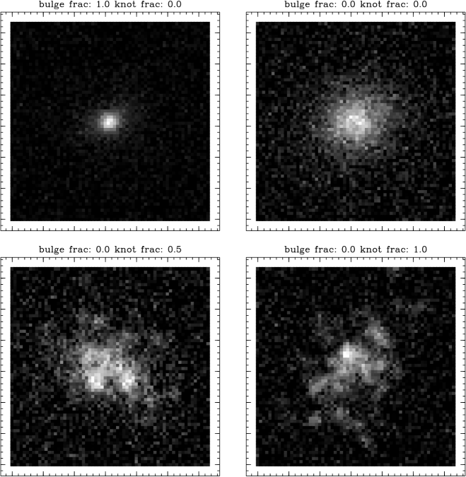
Figure 1.— Example of simulated galaxy images. Each image is a composite of a bulge and disk, plus knots of star formation. The half-light radius is the same for all components, while the fraction of light in each component varies. In the upper left and upper right we show pure bulge and pure disk models, respectively. In the lower left we show a disk with half the light in knots, and in the lower right we show a pure “irregular” galaxy composed entirely of knots. Each model was convolved by a Moffat PSF and pixelized. For demonstration purposes, we here show very large models to make the detailed structure visible; the galaxies used for our shear tests are typically much smaller than the PSF (see figure 2).

In figure 2 we show the distribution of $r_{50}$ for the parametric galaxies, along with the $r_{50}$ for the PSF. Note that most objects had $r_{50}$ significantly smaller than the PSF.

In figure 3 we show the distribution of $S/N$ for the parametric galaxies. Shown are both the true input $S/N$ and the distribution of true $S/N$ after applying a cut at measured $S/N$$>5$. This “true” $S/N$ is that calculated by GALSIM, and is the maximal $S/N$ based on the true model (Jarvis et al., 2016). The measured $S/N$ is noisy and biased (see §8), being derived from a single-Gaussian model, so the cut results in a smooth rolloff in the true $S/N$. This $S/N$ preselection results in a noisy cut on magnitude. The resulting input catalog for metacalibration has a limiting magnitude of COSMOS i-band $\sim$25, but with a significant number of objects removed at brighter magnitudes.

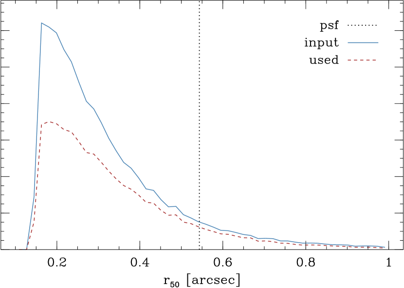
Figure 2.— Distribution of half-light-radius $r_{50}$ in the parametric simulations. The solid line represents the distribution of input $r_{50}$, drawn from fits to COSMOS data. The dashed line represents the $r_{50}$ for objects that passed the initial $S/N>5$ pre-cut. The $r_{50}$ of the PSF is shown as the vertical dotted line.

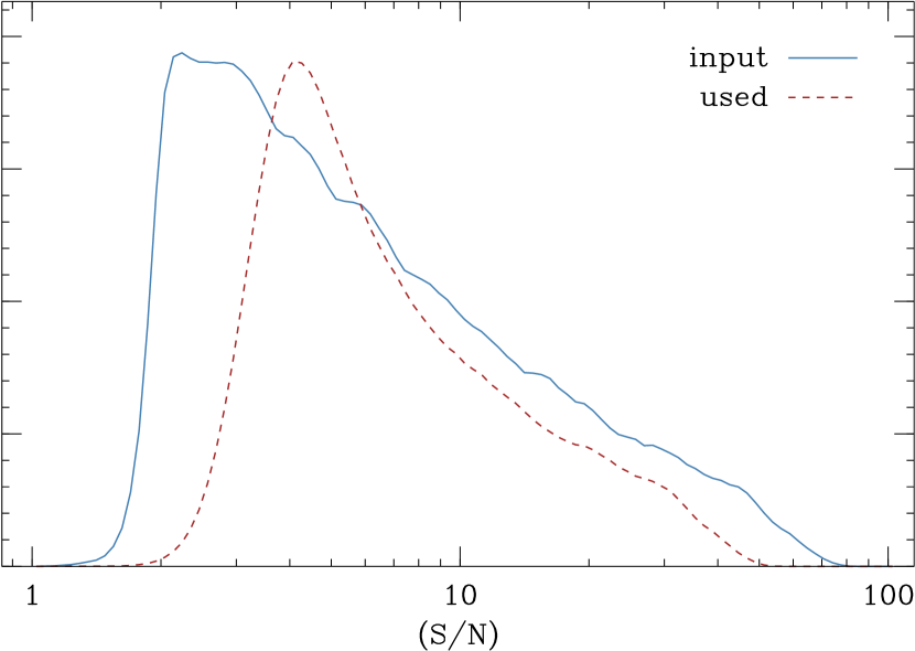
Figure 3.— Distribution of S/N in the parametric simulations. The solid curve represents the true input distribution, the dashed curve represents the objects that passed the initial pre-cut on measured $S/N$$>5$. The measured $S/N$ was biased and noisy, resulting in a smooth selection on true $S/N$. This pre-cut does not sharply cut on magnitude and results in a catalog that is limited at COSMOS i-band magnitude $\sim$25.

6.1.1 Simulated Stars

In order to test the robustness of metacalibration to stellar contamination, we included $\sim$10% stars in the BDK simulation. The stars were simply drawn as PSFs, with the same flux distribution as used for the galaxies. We refer to the simulation with stars as BDK+Stars; the galaxies are identical to those in the BDK simulation, but stars were then included in the analysis.

6.1.2 Preselection

In real data, detections with significance less than $S/N$$\sim 5$ can be spurious, so in practice a threshold must be placed to produce what are considered reliable detections. Such a preselection can produce significant selection biases. A round object has a higher $S/N$ than if it were sheared, and galaxies oriented in the same direction as the PSF have a higher $S/N$ than objects otherwise oriented. Thus a preselection will tend to alter the distribution of ellipticities, which will bias the shear recovery. In particular, if this selection occurs before metacalibration and object fitting, the corrections for selection effects presented in §3 cannot be used.

In the BDK simulation, we generated images with $S/N$ as low as $\sim 2$, as shown in figure 3. In order to test the effect of a preselection, we did not perform the metacalibration process on all images. We applied a preselection on objects with measured $S/N$$>5$, and these objects were removed from the analysis. Then, as discussed in §8.2, we applied further cuts on the measured $S/N$ above this threshold in order to minimize the bias that is due to removal of these galaxies.

6.2. Real-Galaxy Simulations

We designed a second set of simulations to mimic the “real-galaxy” constant shear simulations used in the GREAT3 challenge (Mandelbaum et al., 2014), which used real galaxy images from COSMOS data. The galaxies were drawn from the 23.5 magnitude limited sample distributed with the GALSIM simulation package (Rowe et al., 2015). We generated 1000 different fields in which galaxies were given a constant shear ranging from 0.01 to 0.08, with random orientations.

We implemented two important changes as compared to GREAT3. First, we oriented the galaxies randomly, whereas in GREAT3 the galaxies were placed in pairs rotated by 90 degrees, in order to cancel shape noise. Using paired galaxies has the undesired effect of cancelling some biases that we wish to explore (Jarvis et al., 2016). Second, we used optical aberrations in the PSF designed to match that seen in the Dark Energy Survey data. Similar to GREAT3, we varied the aberrations as Gaussian random variables around a fiducial value. These root-mean-squared variations, in units of waves in the Noll convention (Noll, 1976), are given in table 2. We used a Kolmogorov model for the atmospheric component, such that the overall mean FWHM $\sim 0.9$ arcsec for 0.263 arcsec pixels. Each galaxy was rendered onto a 48 by 48 pixel grid. For this configuration there are significant variations in the PSF ellipticity, but relatively little net ellipticity across the entire simulation. The code used to generate these simulations began as a fork of the GREAT3 public code base, and is freely available online.

Zernike Component	RMS Variation
Defocus	0.13
Astigmatism in Y	0.13
Astigmatism in X	0.14
Coma in Y	0.06
Coma in X	0.06
Trefoil in Y	0.05
Trefoil in X	0.06
Spherical	0.03

Table 2 Root-mean-squared variation for the aberrations in the optical model, in units of waves in the Noll convention, derived from Dark Energy Survey data.

In figure 4 we show the distribution of measured $S/N$ for the COSMOS simulations, as well as for the Bulge+Disk+Knots simulation BDK. Also shown is the distribution of the half-light-radius $r_{50}$ for the two simulations.

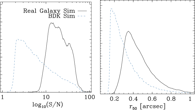
Figure 4.— Distribution of properties in the COSMOS real galaxy simulations. The left panel contains the distribution of measured S/N, while the right panel contains the distribution of half-light-radius from the cosmos catalog for the input galaxies. For comparison, the distributions for the Bulge+Disk+Knots BDK simulations are overplotted as dashed lines.

Note that the galaxies used in the parametric sims presented in §6.1 are much fainter and smaller than those used in the RG simulation. Also note that the RG simulation was relatively expensive compared to the parametric simulations, so we generated fewer galaxies and did not implement any preselection. We thus do not expect the real galaxy simulation to be more challenging than the parametric simulation in every aspect. We include it to directly test the robustness of metacalibration to special properties of real galaxies that may not appear in our Bulge+Disk+Knots simulation, and to test shear recovery using a more realistic PSF.

7. Model Fitting and Metacalibration Operations

We fit the images with a single Gaussian model using the ngmix code. To perform the fit we used an implementation of the “adaptive moments (AM)” algorithm originally presented in Bernstein & Jarvis (2002). We applied no PSF correction. We expected this estimator to respond weakly to a shear, exhibit large model bias, noise bias, and bias due to lack of PSF correction. Note that we also applied metacalibration to a forward-modeling, maximum likelihood estimator; we give some brief results for that method in appendix B.

In order to correct for PSF anisotropy, we reconvolved by a symmetrized version of the PSF. We created this PSF by adding the PSF image to itself, rotated by 90, 120, and 180 degrees. This averaging can result in a Fourier space image that is larger in some dimensions than the original, so we further shrunk the symmetrized PSF in Fourier space. The shrink factor was taken to be $1+2*\delta$, where

$$\delta=\frac{E}{T/2}$$ (29)

Here $E$ is the maximum eigenvalue from the covariance matrix of the best-fit Gaussian. This we divide by half the trace $T$, which is the mean extent of the object. For a purely elliptical PSF, a factor of $1+\delta$ would be sufficient; we conservatively increase the factor to $1+2\delta$ in case the Gaussian fit does not completely capture the asymmetries of the true PSF.

This symmetrization method requires that an image of the PSF is available at the location of the object, which is already a requirement of metacalibration in order to perform deconvolutions. To produce such an image, one must accurately model stars and interpolate to the location of each object, for example as provided by the PSFEx package (Bertin, 2011). Note that instead of using a round reconvolution function, one may instead use the response of the estimator to a PSF shear to address any uncorrected affects of PSF anisotropy (Huff & Mandelbaum, 2017).

All metacalibration image operations were performed using the metacal module from ngmix, which in turn uses GALSIM to perform most image manipulations. We used the correction for correlated noise, as discussed in §4.1

8. Results

In what follows, we will characterize the bias using the standard linear model (e.g. Mandelbaum et al., 2014) with a multiplicative part $m$ and an additive part $c$, such that

$$\left<\gamma_{meas}\right>=(1+m)\gamma_{true}+c.$$ (30)

For the BDK simulations, there was only one shear value (0.02,0.00), and the PSF had ellipticity only in one component (0.000, 0.025). We thus determined $m$ from the first component and $c$ from the second. For the RG simulations, there were many different shears, so the linear model above was fit. We found the multiplicative bias was the same in each component, so we combined them into a single value in the plots and tables below.

In all cases the measured $S/N$ is based on the best-fit Gaussian model (true parameters for the simulated galaxies, such as scale radius or $S/N$, were never used in the analysis). We used a similar definition to that implemented in the GREAT3 simulations (Mandelbaum et al., 2014, equation 16), but replaced the true profile with the model

$$(S/N)^{2}=\frac{1}{\sigma^{2}}\int m(x,y)^{2}dxdy,$$ (31)

where $m$ is the value of the model at location $x,y$, and $\sigma^{2}$ is the variance of the noise in the image. A Gaussian is a poor fit in general, so this measure of the $S/N$ is biased and noisy.

8.1. Metacalibration Responses

In figure 5 we show the measured metacalibration responses for the BDK  simulations. Also shown is the response with the stars included in the BDK+Stars simulation. The distribution of $R$ is quite symmetric in the absence of stellar contamination. We will discuss the affect of stars in §8.2.2.

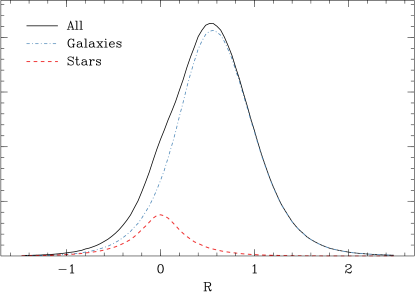
Figure 5.— Distribution of metacalibration responses for galaxies and stars in the BDK+Stars simulation. Stars have mean response close to zero, and thus do not bias the overall shear calibration.

8.2. Shear Recovery

In table 3 we show results for shear recovery in each of our simulations. As was discussed in §6.1.2, we applied a preselection to the BDK simulation at measured $S/N$$>5$, which imposes a selection bias. We thus placed cuts at higher $S/N$ than this threshold, so that the corrections for selection effects presented in §3 could be used accurately. In this table we show results for $S/N$$>10$. For the RG simulation we did not apply a preselection.

Sim	$m$	$c_{1}$	$c_{2}$
	$[10^{-3}]$	$[10^{-5}]$	$[10^{-5}]$
RG	$0.22\pm 0.58$	$2.6\pm 2.9$	$2.2\pm 2.9$
BDK	$0.03\pm 0.31$	-	$-0.15\pm 0.62$
BDK+Stars	$0.01\pm 0.32$	-	$-0.08\pm 0.63$

Table 3 Metacalibration results for each image simulation described in §6 and table 1. For each simulation, a cut was placed at $S/N$$>10$, and corrections were applied for selection effects (see table 4 for more results on selections). A single Gaussian was fit to the observed object, with no PSF correction applied. No multiplicative or additive bias was detected in any case. Stellar contamination at the level of 10% increases the noise in the recovered shear by $\sim 2-3$% but does not introduce a significant bias.

Using metacalibration we found no significant multiplicative or additive biases. Without applying the metacalibration responses, the multiplicative bias $m$ was of order 50% for all simulations.

8.2.1 Results with Selection Effects

In table 4 we show the results for different $S/N$ threshold cuts in the BDK simulations. We show the recovered bias with and without corrections for selection effects. These results are also shown graphically in figures 6 and 7. The cuts were all placed above the preselection at $S/N$$>5$ to guarantee the validity of the corrections.

	Uncorrected for Selection		Corrected for Selection
Selection	$m$	$c$	$m$	$c$
	$[10^{-3}]$	$[10^{-5}]$	$[10^{-3}]$	$[10^{-5}]$
$\mbox{$S/N$}>7$	$+15.55\pm 0.34$	$+0.80\pm 0.68$	$+0.55\pm 0.34$	$+0.79\pm 0.67$
$\mbox{$S/N$}>10$	$+3.78\pm 0.31$	$-0.15\pm 0.62$	$+0.03\pm 0.31$	$-0.15\pm 0.62$
$\mbox{$S/N$}>13$	$-1.46\pm 0.31$	$+0.27\pm 0.63$	$+0.03\pm 0.31$	$+0.27\pm 0.63$
$\mbox{$S/N$}>16$	$-4.58\pm 0.33$	$+0.44\pm 0.67$	$+0.26\pm 0.34$	$+0.44\pm 0.67$
$\mbox{$S/N$}>19$	$-8.33\pm 0.36$	$+0.17\pm 0.73$	$+0.05\pm 0.37$	$+0.18\pm 0.73$

Table 4 Metacalibration results for the BDK simulation with various cuts on signal-to-noise ratio $S/N$. Results are shown with and without corrections for selection effects.

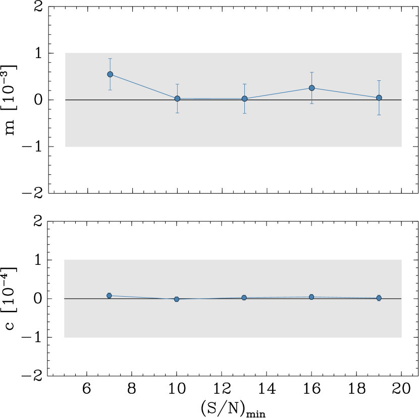
Figure 6.— Multiplicative (upper panel) and additive bias (lower panel) in the BDK simulation after applying threshold selections in the measured signal-to-noise ratio $S/N$. The filled gray region represents the target accuracy.

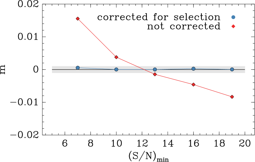
Figure 7.— Same as the top panel of figure 6, but now additionally showing the multiplicative bias without corrections for selection effects. The bias without correction for selection effects is represented as red diamonds. The bias after correction for selection effects is represented as blue circles. The filled gray region represents the target accuracy.

We measured and corrected for a significant multiplicative selection bias in each case. These biases are generally well above our desired part-in-a-thousand accuracy. After correction, we found that the multiplicative bias was less than a part in a thousand in all cases. We did not find any additive selection biases, which suggests that our procedure of reconvolving by a symmetrized PSF was sufficient for these simulations.

8.2.2 Results with Stellar Contamination

Results including 10% stars in the BDK+Stars simulation are shown in table 3. We did not detect any additional bias after including stars. The noise in the recovered shear did, however, increase by $\sim 2-3$%.

Metacalibration is robust to stellar contamination if the PSF is well characterized. Images consistent with a PSF will not, in the mean, respond to the shear applied during the metacalibration process. Measurement on stars also yields zero average shape as long as the PSF correction is sufficiently accurate: our use of a symmetrized PSF (see §7) appears to be sufficient in this case. In figure 5 we show the measured response $R$ for stars and galaxies. Indeed we see that for stars, the $R$ is noisy but consistent with zero. Thus, in the mean, stars contribute zero to both the estimator and response, leaving equation 4 unbiased.

If the additional variance is tolerable, it may be useful to include stars in a shear analysis if the PSF is sufficiently well known. Attempting to remove faint stars from a sample is a noisy procedure, likely to induce selection effects. These can be controlled using the corrections derived in §3, but only if the selection is also repeated based on quantities measured on sheared images, so the corrections can be calculated. If the selection must be performed outside of the metacalibration process, it may be better to avoid it altogether.

For accurate interpretation of the signal, it is important to weight by the metacalibration response terms in order to obtain the correct redshift distribution (see §5 for more discussion of weighted means). It is also desirable that the redshift estimates for stars be close to zero, so that the weighted redshift distribution is minimally contaminated.

8.2.3 Effects of Missing Data

The Fourier transforms used to perform the metacalibration convolutions cannot accommodate missing data. In real data there are features in the image, however, such as bad pixels and columns, and cosmic rays that cannot be used for object measurement. This can be dealt with easily when the galaxy model is fit simultaneously to postage stamps drawn from all available observing epochs and bands (e.g. Jarvis et al., 2016). If the epochs are spatially offset, such that the object does not always appear at the same location in the image, then a small fraction of images should be affected by missing data such as bad pixels. In that case, data deemed problematic can simply be left out of the fit.

If only a single image is available, one may wish to replace the missing data. To test this scenario, we chose to replace the missing data with the value from the best fit Gaussian model. Using a better model would be preferred; this may be considered a worst-case scenario.

We ran a simulation in which 10% of the images had bad pixels or bad columns. We found that the model replacement worked well for single bad pixels. For bad columns we found a large additive $e_{1}$ bias, as well as a multiplicative bias of a few parts in a thousand. However, this bias disappeared if we introduced a compensatory “bad column” at 90 degree rotation about the center of the image, restoring symmetry to the image. Again, we wish to emphasize that such a procedure may not be necessary when there are many images available for fitting.

8.2.4 Noise Degredation Due to Correlated Noise Corrections

As a result of the noise added to correct for correlated noise (see §4.1), the $S/N$ of the measurements after the metacalibration procedure are reduced by $\sqrt{2}$, but this not a severe limitation. For faint galaxies, which dominate the sample, the shape measurement noise is comparable to the intrinsic shape noise, so one might expect the increase in effective shear noise to be less than $\sqrt{2}$.

We performed a test where the mean shear was calculated in a simulation, with the correlated noise correction. This was compared to a “perfect” metacalibration procedure without correlated noise. To accomplish this, we added noise after the metacalibration image manipulations were performed, rather than before. In both cases we placed a cut at S/N$\ >10$. For the simulations described in §6.1 and the fitting used in §7, we found that the uncertainty in the shear recovery was increased by $\sim$20%. Note that one may be tempted to decrease the $S/N$ cut to recover objects that have a lower $S/N$ after the additional noise is added, but we find that including objects with $S/N$ $<10$ actually increases the variance. This can also be seen in the results shown in table 4. We found this to be true even when inverse variance weighting was introduced.

For correlation function measurements over large scales, such as shear-shear correlations, sample-variance will dominate and this 20% increase will be relatively unimportant. Nevertheless, we consider it worthwhile to explore alternative corrections that do not involve adding significant noise.

9. Weak Shear Approximation

In deriving the response terms in §3, we assumed the shear was small, so that the response of the estimator to a shear was linear. This approximation will break down at higher shears. We expect the multiplicative bias to have the following generic form (Bernstein et al., 2016):

$$B(\gamma)=m+\alpha\gamma^{2}+O(\gamma^{4})$$ (32)

We tested the bias from nonlinearity using both the BDK image simulations and a “toy model,” inspired by that used in (Bernstein & Armstrong, 2014). For the BDK image simulations, we ran tests with shears of 0.06 and 0.10, in addition to the 0.02 discussed above.

For the toy model we drew ellipticities from the distribution given in equation 27 and added constant shear analytically using the standard shear transformation equations (Seitz & Schneider, 1997). We then multiplied by a bias factor of 0.6 and added Guassian noise to each ellipticity component with scatter of 0.2. We truncated the total ellipticity to be less than unity, making the noise effectively non-Gaussian. We performed metacalibration operations by analytically shearing the shapes. Note that we did not shear the noise, so sheared noise effects as seen in the image simulations are not present.

In figure 8 we show the results. Fitting the bias model in equation 32, we found $m\sim 0$ and $\alpha\sim 1$ for the toy model. For the image simulations we found $m\sim 0$ and $\alpha\sim 0.6$. We note that Bernstein et al. (2016) also found that the value of $\alpha$ depended on the type of simulation used, with values for $\alpha$ as high as 2. Taking the value of $\alpha$ from the image simulation, we find that the nonlinearity in this simulation becomes greater than our part-in-a-thousand goal for shears greater than about 0.04. Using $\alpha=1$ from the toy model, we reach the threshold for shears higher than about 0.03.

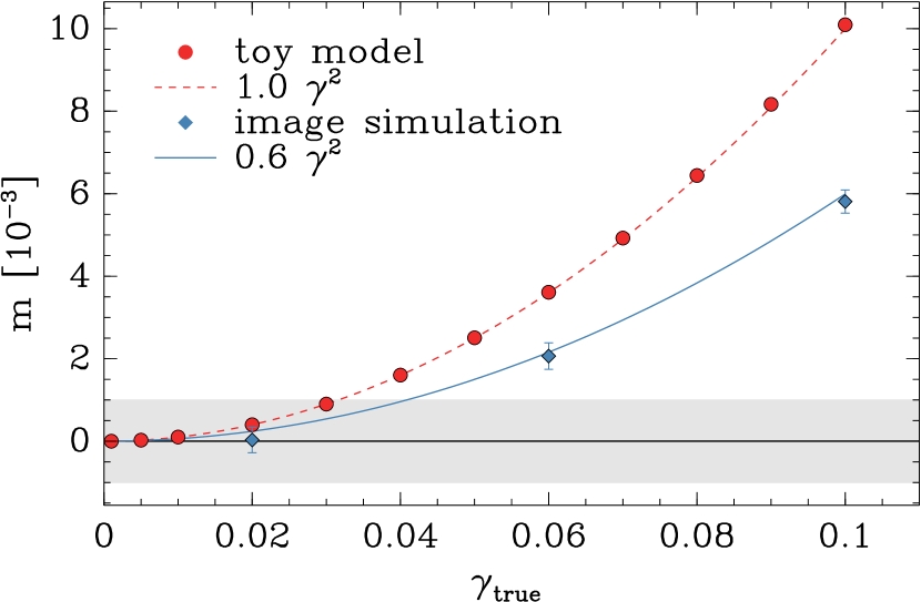
Figure 8.— Multiplicative bias as a function of applied shear in two types of simulations. The circles represent the results for the toy simulation presented in the text. The diamonds represent results for the parametric BDK image simulations. For the toy simulation, the bias scales with $\gamma^{2}$. For the image simulation the bias scales as $0.6\gamma^{2}$. The gray region represents the target accuracy.

Following the discussion in Bernstein et al. (2016), we expect the bias on a cosmic shear measurement to be approximately $1+3\alpha\sigma_{\gamma}^{2}$, with a shear variance of $\sigma_{\gamma}^{2}\sim 0.02^{2}$. For the $\alpha=0.6$ found in the image simulations, the bias would be about $7.2\times 10^{-4}$. For $\alpha=1$, the bias would be be about $1.2\times 10^{-3}$, exceeding our desired accuracy and requiring some correction. As pointed out by Bernstein et al. (2016), this correction does not require great precision. If the bias were determined at the $\sim 40$% level for $\alpha=1$, the shear could be recovered accurately with 95% confidence. More care may be required for measurements of higher shear, such as tangential shear measurements near the centers of galaxy clusters. We will explore strategies to mitigate this potential bias in a future work.

10. Computation Time

metacalibration involves performing image manipulations five times, one for the zero shear, but reconvolved image, and four for each of the sheared images. We then perform image fitting on each of these images.

The total computation time per object was approximately 0.2 seconds. In our tests the time was dominated by the image manipulations, primarily the Fourier transforms used for convolutions. The image manipulations dominated partly because we used the fast ngmix code; fitting each image took only about 0.001 seconds, so about 0.005 to fit all five images. For slower fitting codes, the metacalibration manipulations may be subdominant.

It may be that further optimization is possible. For example, a code that works entirely in Fourier space could avoid rendering the reconvolved image in real space.

11. Summary and Future Work

We introduced a formalism for metacalibration to calculate shear response corrections, including corrections for selection effects. We developed a simple empirical correction for the correlated noise associated with the metacalibration procedure.

We tested the formalism using simulations based on real galaxy images, as well as challenging parametric simulations that included preselection effects and stellar contamination. We applied a range of cuts on the object $S/N$, inducing significant selection affects. In all cases we recovered the input shear to better than a part in a thousand.

Metacalibration compares favorably with other shear measurement techniques. At the time of writing, the only technique with demonstrated accuracy close to metacalibration, without reliance on calibration from simulations, and which accurately addresses selection effects, is BFD (Bernstein et al., 2016). metacalibration has been tested using more challenging simulations and has proved more accurate. Unlike BFD, Metacalibration does not rely on significant prior information about galaxy properties. On the other hand, in our current implementation we add extra noise to deal with correlated noise effects. This extra noise increases the uncertainty in the shear recovery by about 20% in our tests. The relative increase in noise should be smaller for studies that are sample-variance limited, such as shear-shear correlations on large scales. Nevertheless, we have identified the development of a more precise correlated noise correction as a priority going forward.

In order to reach part-in-a-thousand accuracy in real data, there are a number of additional challenges to be addressed. These challenges are shared with other shear measurement techniques. We think the most important are the effects of overlapping objects and the limitations of current image processing techniques. The accurate determination of the PSF is also fundamental, but we do not address that here.

Biases in the image processing pipeline that identifies image artifacts, determines the background light, identifies unique detections, and assigns light to objects will potentially produce biases in the shear recovery. Image artifacts may not be properly corrected for, or masked. In crowded regions such as galaxy clusters, the pipeline may fail to determine the background accurately. The metacalibration process may not accurately determine the shear response in these cases.

In crowded regions the detection algorithm may fail to identify all the unique objects, even those brighter than the detection threshold, because objects overlap significantly on the sky. The Metacalibration procedure will correctly estimate the shear response for blended objects, as long as the presence of neighbors does not result in an instability in the measurement process. This is sufficient for blends at the same redshift, but for blends at different redshift, this combined shear response has no simple interpretation because each object will experience a different shear. Ideally, we would identify the unique objects and assign a fraction of the light in each pixel to each object. Then separate shear responses would be measured for each object, and redshifts of the objects would be determined, at least statistically.

There will also be large numbers of faint galaxies that are not bright enough to exceed the detection threshold. This is an important source of bias when using simulations to calibrate the shear (see e.g. Hoekstra et al., 2017), but we have not yet tested how this will affect metacalibration. These objects will be included at some level in the metacalibration shear response measured for brighter galaxies, and will contaminate the light used for flux and color determination. The concern in this case is the same as for the bright blends mentioned above: unique objects must be identified and the redshift distribution determined in order to properly interpret the shear measurement. The presence of unidentified neighbors will complicate this process. Going forward, it is imperative to assess the importance of this effect on both the shear response measurement and redshift determination.

It may be possible to address these issues by inserting artificial galaxy images into the data using something like the BALROG framework (Suchyta et al., 2016), followed by rerunning processing pipelines, including shear estimation. BALROG uses the original images as the basis, so all the features of real observations need not be simulated. The approach is particularly applicable to studying the effects of blending, undetected objects, and image artifacts.

The formalism we have developed recovers a weighted average of the shear, and this weighting is known, being the same responses used to calibrate the shear estimate. In this work we only tested the simplest case of constant shear. When using metacalibration in real data, where the shear and response vary across the sky, it will be important to accurately propagate this weighting, for example when inferring the redshift distribution of a source population.

Appendix A Alternative Methods for Correlated Noise Correction

A.1. Correction using GALSIM Methods

With guidance from the GALSIM developers, we attempted to use the GALSIM noise isotropization and whitening functionality to correct the correlated noise. Isotropization enforces four-fold symmetry, introducing minimal extra noise, while whitening completely whitens the image, introducing significant extra noise. However, neither of these methods improved the shear recovery in our simulations. It may be that some aspects of the metacalibration procedure invalidate the assumptions behind these correction methods.

A.2. Detrending the Correlated Noise Bias

A.2.1 Expected Scaling of the Bias with Noise Level

The bias in the ellipticity that is due to correlated noise should scale with the noise correlation function, and thus the square of the noise level in the image $n^{2}$ (Kaiser, 2000; Hirata, 2016). As discussed in §4, this bias will propagate into the response. We can write the observed $R_{o}$ as a contribution from both the actual response $R$ and a noise term $R_{\eta}$

$$R_{o} =\mbox{\boldmath$R$}+\mbox{\boldmath$R_{\eta}$}$$

$$=\mbox{\boldmath$R$}+An^{2}.$$ (A1)

A.2.2 Detrending Correction Scheme

We add a small amount of noise to the image such that $n\rightarrow n+\Delta n$. If we then run the new image through the metacalibration process, we can measure $R^{\mathrm{before}}$, a response that will include correlated noise effects. We can write this observed response as

$$\mbox{\boldmath$R_{o}$}^{\mathrm{before}} =\mbox{\boldmath$R$}+A(n+\Delta n)^{2}$$

$$\simeq\mbox{\boldmath$R$}+An^{2}+2An\Delta n$$ (A2)

where we have dropped terms of order $(\Delta n)^{2}$ and higher. In equation A.2.2, $R$ is the response at noise $n+\Delta n$ in the absence of correlated noise.

We can also add identical noise after the original image has been run through metacalibration, and measure $R^{\mathrm{after}}$. The response when adding noise after metacalibration does not suffer any additional bias due to correlated noise:

$$\mbox{\boldmath$R_{o}$}^{\mathrm{after}} =\mbox{\boldmath$R$}+An^{2}.$$ (A3)

The difference between these responses is then

$$\Delta\mbox{\boldmath$R$} \equiv\mbox{\boldmath$R_{o}$}^{\mathrm{before}}-\mbox{\boldmath$R_{o}$}^{\mathrm{after}}$$

$$\simeq 2An\Delta n.$$ (A4)

We propose the following procedure to correct for correlated noise:

1. Calculate $\Delta\mbox{\boldmath$R$}$ for a series of noise offsets $\Delta n$.

2. Average $\Delta\mbox{\boldmath$R$}$ over all objects for each noise offset.

3. Perform a linear fit to $\Delta\mbox{\boldmath$R$}$ vs. $2n\Delta n$ to find the coefficient $A$.

4. Apply a mean correction for correlated noise given by

   $$R_{\eta} \simeq An^{2}.$$ (A5)

If the noise varies between observations, we can apply a correction based on the mean variance $A\langle n^{2}\rangle$.

A.2.3 Measurements of the detrending Parameters

We measured $\Delta R$ vs $2n\Delta n$ to find the coefficient $A$. In figure 9, we show this fit for the RG simulation. The trend is well fit by a linear model, as expected, with a slope $A\simeq$$-1.11$, implying a correction $An^{2}\simeq$ $-0.0694$ for this simulation.

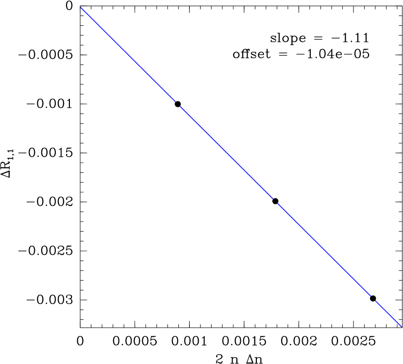
Figure 9.— Trend of $\Delta R_{1,1}$ with $2n\Delta n$ for the real galaxy simulation. $n$ is the original noise level and $\Delta n$ is the additional noise added. The trend is linear as predicted.

A.2.4 Using a Random Subset To Calculate Detrending Corrections

Measuring the detrending parameters requires extra computations, at least a factor of three to fit the linear parameters given in §A.2, and a factor of four if an additional point is used to check for possible nonlinearity. These extra computations could be expensive for large surveys.

However, the detrending parameters are more precisely measured than the shear itself. Here we explore the precision of the recovered shear using smaller subsets of the object catalog to measure the detrending parameters, and applying the corrections to the full sample. In Table 5 we show the shear recovery parameters for various subset sizes for the BDK simulation described in §8

We find that a relatively small sample can be used to determine the correlated noise correction. Calculating the detrending terms for 10% of the sample leads to only 0.3% extra variance in the recovered shear, and using 1% of galaxies leads to only 4.4% increase in variance.

To calculate these numbers, we have assumed the extra uncertainty is added quadratically with the uncertainty measured using all galaxies to estimate the detrending parameters; e.g for the first row, we have added approximately 30% quadratically with the measured uncertainty, resulting in a net increase of 4.4%.

It is important to use a truly random subset of the population to determine the corrections, including a fair sample of stars and other contaminants, and a representative amount of pixel level masking. If a particular aggregate shear measurement involves a selection, this selection must also be applied to the random subset.

A.2.5 Performance of the detrending method

We found that this method did not work as well as the fixnoise method described in §4.1. We detected a remaining bias of $m\sim 2\times 10^{-3}$ in the RG simulations.

A.3. Simulating Models

In this method, we generated model images with the correct noise level corresponding to each real image. We then measured the response of the noise that is due to the convolutions and shears used in metacalibration, with noise added before and after the metacalibration procedure.

The measurement with correlated noise will be the sum of the response without correlated noise plus the response of the correlated noise field,

$$\mbox{\boldmath$R^{model}_{\eta}$}=\mbox{\boldmath$R^{model}$}+\mbox{\boldmath$R_{\eta}$}.$$ (A6)

This measurement is quite noisy for a single galaxy, but we can estimate the mean correlated noise response for an ensemble of galaxies,

$$\langle\mbox{\boldmath$R_{\eta}$}\rangle=\langle\mbox{\boldmath$R^{model}_{\eta}$}\rangle-\langle\mbox{\boldmath$R^{model}$}\rangle.$$ (A7)

Each entry used in this average corresponds to the best-fit model and noise properties for a galaxy in the sample.

The response $R_{\eta}$ can be subtracted to recover an estimate of the mean response without correlated noise,

$$\langle\mbox{\boldmath$R$}\rangle=\langle\mbox{\boldmath$R_{o}$}\rangle-\langle\mbox{\boldmath$R_{\eta}$}\rangle.$$ (A8)

We detected significant bias using both exponential and Gaussian models for the galaxy. We found a remaining bias of $m\sim 4\times 10^{-3}$ in the RG simulations.

Subset Size	Extra Error
1%	4.4%
5%	0.8%
10%	0.3%

Table 5 Additional variance in the recovered shear using differently sized subsets to estimate the detrending corrections. Values were obtained from 100 bootstrap samples.

Appendix B Metacalibration Using Maximum-likelihood Forward Modeling

In §8 we discussed in detail the results for a moment based fitting method using adaptive moments (AM), with no explicit PSF correction. We also performed tests using a forward-modeling maximum likelihood method. In this method we fit a single Gaussian to the PSF and then fit a Gaussian to each object, convolved analytically by the Gaussian PSF model. This method should be more sensitive because the PSF is accounted for in the modeling, although imperfectly. We applied smooth priors to the likelihood for each parameter in the model in order to ensure a stable fit, but these priors were not tuned to match the true parameters of the simulated galaxies.

In the Bulge+Disk+Knots simulation, we found this method to perform equally as well as AM, but with some interesting differences. The method is indeed more sensitive: as shown in figure 10, the distribution of the response has a narrow peak near 0.7, corresponding to disk-dominated galaxies with a high $S/N$, with a tail to low response from a mix galaxies with low $S/N$. Note also that the expected value for perfect response for this estimator is unity, whereas for AM it would be approximately twice as large because the estimator for AM is a distortion style ellipticity rather than a reduced shear style ellipticity. However, we do not see correspondingly large decrease in the variance of the shear estimator, so it is not clear whether this increased sensitivity is necessarily an advantage.

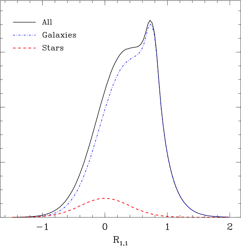
Figure 10.— Distribution of shear response in the Bulge+Disk+Knots simulations for a shear estimator based on forward-modeling maximum likelihood fitting. The colors and line styles are the same as that used in figure 5.

We also note that the distribution of response for the forward-modeling estimator is less symmetric than for AM without PSF correction (see figure 5), but this did not bias the shear recovery. We see that the distribution of response for stars is still quite symmetric about zero for this estimator.

It was noted in Huff & Mandelbaum (2017) that for some very noisy estimators, the resulting complex distribution of response can be problematic. For this reason, we suggest that practitioners explore the performance of their chosen estimator in simulations before applying it to real data.

References

- Bernstein (2010) Bernstein G. M., 2010, MNRAS, 406, 2793
- Bernstein & Armstrong (2014) Bernstein G. M., Armstrong R., 2014, MNRAS, 438, 1880
- Bernstein & Jarvis (2002) Bernstein G. M., Jarvis M., 2002, AJ, 123, 583
- Bernstein et al. (2016) Bernstein G. M., Armstrong R., Krawiec C., March M. C., 2016, MNRAS, 459, 4467
- Bertin (2011) Bertin E., 2011, in Evans I. N., Accomazzi A., Mink D. J., Rots A. H., eds, Astronomical Society of the Pacific Conference Series Vol. 442, Astronomical Data Analysis Software and Systems XX. p. 435
- Clowe et al. (2006) Clowe D., Bradač M., Gonzalez A. H., Markevitch M., Randall S. W., Jones C., Zaritsky D., 2006, ApJ, 648, L109
- Fenech Conti et al. (2017) Fenech Conti I., Herbonnet R., Hoekstra H., Merten J., Miller L., Viola M., 2017, MNRAS, 467, 1627
- Heymans et al. (2013) Heymans C., et al., 2013, MNRAS, 432, 2433
- Hirata (2016) Hirata C., 2016, in preparation
- Hirata et al. (2004) Hirata C. M., et al., 2004, MNRAS, 353, 529
- Hirata et al. (2007) Hirata C. M., Mandelbaum R., Ishak M., Seljak U., Nichol R., Pimbblet K. A., Ross N. P., Wake D., 2007, MNRAS, 381, 1197
- Hoekstra & Jain (2008) Hoekstra H., Jain B., 2008, Annual Review of Nuclear and Particle Science, 58, 99
- Hoekstra et al. (2017) Hoekstra H., Viola M., Herbonnet R., 2017, MNRAS, 468, 3295
- Huff & Mandelbaum (2017) Huff E., Mandelbaum R., 2017, preprint, (arXiv:1702.02600)
- Huterer et al. (2006) Huterer D., Takada M., Bernstein G., Jain B., 2006, MNRAS, 366, 101
- Ivezic et al. (2008) Ivezic Z., et al., 2008, preprint, (arXiv:0805.2366)
- Jarvis et al. (2016) Jarvis M., et al., 2016, MNRAS, 460, 2245
- Jee et al. (2016) Jee M. J., Tyson J. A., Hilbert S., Schneider M. D., Schmidt S., Wittman D., 2016, ApJ, 824, 77
- Johnston et al. (2007) Johnston D. E., et al., 2007, preprint, (arXiv:0709.1159)
- Kaiser (2000) Kaiser N., 2000, ApJ, 537, 555
- Kaiser et al. (1995) Kaiser N., Squires G., Broadhurst T., 1995, ApJ, 449, 460+
- Kilbinger et al. (2013) Kilbinger M., et al., 2013, MNRAS, 430, 2200
- Lackner & Gunn (2012) Lackner C. N., Gunn J. E., 2012, MNRAS, 421, 2277
- Laureijs et al. (2011) Laureijs R., et al., 2011, preprint, (arXiv:1110.3193)
- Mandelbaum et al. (2006) Mandelbaum R., Seljak U., Kauffmann G., Hirata C. M., Brinkmann J., 2006, MNRAS, 368, 715
- Mandelbaum et al. (2014) Mandelbaum R., et al., 2014, ApJS, 212, 5
- Melchior & Viola (2012) Melchior P., Viola M., 2012, MNRAS, 424, 2757
- Melchior et al. (2014) Melchior P., Sutter P. M., Sheldon E. S., Krause E., Wandelt B. D., 2014, MNRAS, 440, 2922
- Miller et al. (2013) Miller L., et al., 2013, MNRAS, 429, 2858
- Moffat (1969) Moffat A. F. J., 1969, A&A, 3, 455
- Noll (1976) Noll R. J., 1976, Journal of the Optical Society of America (1917-1983), 66, 207
- Okura & Futamase (2016) Okura Y., Futamase T., 2016, ApJ, 827, 138
- Refregier & Amara (2014) Refregier A., Amara A., 2014, Physics of the Dark Universe, 3, 1
- Refregier et al. (2012) Refregier A., Kacprzak T., Amara A., Bridle S., Rowe B., 2012, MNRAS, 425, 1951
- Rowe et al. (2015) Rowe B. T. P., et al., 2015, Astronomy and Computing, 10, 121
- Schneider et al. (2015) Schneider M. D., Hogg D. W., Marshall P. J., Dawson W. A., Meyers J., Bard D. J., Lang D., 2015, ApJ, 807, 87
- Scoville et al. (2007a) Scoville N., et al., 2007a, ApJS, 172, 38
- Scoville et al. (2007b) Scoville N., et al., 2007b, ApJS, 172, 150
- Seitz & Schneider (1997) Seitz C., Schneider P., 1997, A&A, 318, 687
- Sheldon et al. (2009) Sheldon E. S., et al., 2009, ApJ, 703, 2217
- Spergel et al. (2015) Spergel D., et al., 2015, preprint, (arXiv:1503.03757)
- Suchyta et al. (2016) Suchyta E., et al., 2016, MNRAS, 457, 786
- Takada (2010) Takada M., 2010, in Kawai N., Nagataki S., eds, American Institute of Physics Conference Series Vol. 1279, American Institute of Physics Conference Series. pp 120–127, doi:10.1063/1.3509247
- The Dark Energy Survey Collaboration (2005) The Dark Energy Survey Collaboration 2005, ArXiv Astrophysics e-prints,
- Troxel & Ishak (2015) Troxel M. A., Ishak M., 2015, Phys. Rep., 558, 1
- Tyson et al. (1984) Tyson J. A., Valdes F., Jarvis J. F., Mills A. P., 1984, ApJ, 281, L59
- Zhang (2008) Zhang J., 2008, MNRAS, 383, 113
- Zhang et al. (2015) Zhang J., Luo W., Foucaud S., 2015, J. Cosmology Astropart. Phys, 1, 024
- Zhang et al. (2017) Zhang J., Zhang P., Luo W., 2017, ApJ, 834, 8
- Zuntz et al. (2013) Zuntz J., Kacprzak T., Voigt L., Hirsch M., Rowe B., Bridle S., 2013, MNRAS, 434, 1604