Metacalibration: Direct Self-Calibration of Biases in Shear Measurement

Abstract

One of the primary limiting sources of systematic uncertainty in forthcoming weak lensing measurements is systematic uncertainty in the quantitative relationship between the distortions due to gravitational lensing and the measurable properties of galaxy images. We present a statistically principled, general solution to this problem. Our technique infers multiplicative shear calibration parameters by modifying the actual survey data to simulate the effects of a known shear. It can be applied to any shear estimation method based on weighted averages of galaxy shape measurements, which includes all methods used to date for shear estimation with real data. Use of the real images mitigates uncertainty due to unknown galaxy morphology, which is a serious concern for calibration of shear estimates based on image simulations. We test our results on simulated images from the GREAT3 challenge, and show that the method eliminates calibration biases for several different shape measurement techniques at the level of precision measurable with the GREAT3 simulations (a few tenths of a percent).

1. Introduction

Accurate measurement of weak gravitational lensing offers the most direct probe of the dark sector of the universe (e.g., Bartelmann & Schneider 2001; Refregier 2003; Schneider 2006; Hoekstra & Jain 2008; Massey et al. 2010; Weinberg et al. 2013). Weak lensing measurements are thus a core part of the international cosmology program, and a key science driver for several wide-field astronomical imaging cameras and associated surveys – the Kilo Degree Survey (de Jong et al. 2015), the Dark Energy Survey (Flaugher 2005), the Hyper Suprime-Cam and associated survey (Miyazaki et al. 2012), LSST (LSST Science Collaborations & LSST Project 2009), Euclid (Laureijs et al. 2011), and WFIRST (Spergel et al. 2015).

Despite this investment, the weak lensing community has more work to do in order to ensure that the algorithms for inferring shear are unbiased at the required levels to avoid systematic errors from dominating over the statistical errors. One of the largest such systematic error sources is the shear calibration bias, the quantitative relationship between the true gravitational lensing shear and its observables as estimated from the ensemble of galaxies in the survey.

In the weak shear limit that is most relevant for wide-field cosmology, the gravitational lensing signal can be described as a linear transformation $\boldsymbol{A}\mathbf{x}_{\rm true}=\mathbf{x}_{\rm obs}$ between the lensed and unlensed image coordinates, parameterized by two shears $(\gamma_{1},\gamma_{2})$ and a convergence $\kappa$

$$\boldsymbol{A}=\begin{pmatrix}1+\kappa+\gamma_{1}&\gamma_{2}\\ \gamma_{2}&1+\kappa-\gamma_{1}\end{pmatrix}$$ (1)

. The major observable effect of weak lensing is to perturb the measured ellipticities $\mathbf{e}=(e_{1},e_{2})$ of galaxies. At large separations, these shapes no know preferred direction, so the mean $\mathbf{e}$ should vanish over a wide enough field. Weak lensing studies exploit this intrinsic symmetry, and search for spatially coherent anisotropies in the ensemble of observed galaxy shapes arising from lensing distortions produced by foreground matter.

The effects of the shear and convergence on this observable cannot be straightforwardly distinguished, so the fundamental quantity constrained by lensing is the reduced shear

$$g=\frac{\gamma}{1-\kappa}.$$ (2)

The responses of individual galaxy images to $g$ vary depending on the choice of ellipticity measure and the intrinsic shape and orientation of each galaxy. Lensing studies rely on ensemble averages of galaxy ellipticities, and the shears are weak enough that these ensemble averages usually respond linearly to an applied (reduced) shear, so it is conventional to define the multiplicative shear calibration and additive bias parameters as

$$\langle\mathbf{e}\rangle=(1+m)\langle\mathbf{g}\rangle+\mathbf{c}$$ (3)

where $\mathbf{e}$ and $\mathbf{g}$ are ensemble-averaged shears and ellipticity measures, respectively. Generally, $\mathbf{c}$ is a result of measurement biases (such as an incomplete correction for the point-spread function) that introduce a preferred direction in the image plane. It can in principle be known or removed with sufficient knowledge of the experiment. $m$ depends in part on the ensemble of (unobserved) galaxy properties, so it is impossible in principle to know exactly a priori (though Bernstein & Armstrong 2014 show how to derive this information for their proposed shear estimator, which does not make use of an ensemble average over ellipticities, from deeper calibration fields).

In practice, a nonlinear response generically introduced by the algorithms used for measurement of $\boldsymbol{e}$ can introduce both multiplicative and additive biases in a manner that interacts with the unknown true ensemble properties of galaxies (Massey et al. 2007b; Zhang & Komatsu 2011), and are very difficult to predict from first principles. For this reason, the weak lensing community has organized a series of blind measurement challenges, where participants attempted to extract an unkown lensing signal from simulated images. The earliest of these were the first two Shear TEsting Programmes (Heymans et al. 2006; Massey et al. 2007a, STEP1, STEP2). The results made two things clear: that lensing measurement algorithms needed to improve in order to avoid being systematics-dominated, and that shear measurement was sufficiently complex that successive simulation challenges should focus on a subset of the issues.

The next round of simulation challenges – GREAT08, GREAT10, and GREAT3 (Bridle et al. 2009; Kitching et al. 2013; Mandelbaum et al. 2015) – embraced a narrower focus and saw significant performance improvements. They also drove improvements in our understanding of various sources of bias in shear estimation, which is of use in future algorithmic development. The best-performing algorithms from the most recent challenge, GREAT3, reduced $m$ and $c$ to levels approaching those needed for the most ambitious planned lensing measurements, albeit with simulations that did not include all the features of real data.

While this was certainly good news, the narrowed focus of the GREAT challenges necessarily left some of the most important sources of lensing calibration bias untouched. Remaining issues of significant concern include biases resulting from:

• object detection and selection

• deblending

• wavelength-dependent effects

• instrumental defects and nonlinearities

• star-galaxy separation

• non-white pixel noise

• cosmic rays and other image artifacts

• redshift-dependent calibration biases

• shear estimation for low-resolution and/or low signal-to-noise ratio ($<12$) galaxies

The impact of these factors depends strongly on the specifics of the experiment. For this reason, shear calibration in current and future experiments relies heavily on simulations designed to match the properties of each experiment (Hildebrandt et al. 2016; Jarvis et al. 2016). Such external simulations are always limited in their realism: accurately modeling everything relevant about the experiment turns out to be extremely difficult. Showing that a given simulation suite is adequate for calibrating a lensing measurement is a formidable challenge in its own right (c.f. the Ultra Fast Image Generation simulations described in Bergé et al. 2013, or the calibration simulations used for the KiDS weak lensing cosmology in Fenech Conti et al. 2016).

The method outlined in this paper is motivated by the observation that introducing a synthetic shear signal into real data is much easier than building a realistic comprehensive first-principles simulation suite. While in practice the need for accurate simulations of the ensemble of galaxy images is sometimes met by relying on images from external deep fields like the Hubble Space Telescope’s COSMOS survey (Koekemoer et al. 2007; Scoville et al. 2007b, a), the deeper fields needed for calibration of future surveys like LSST and WFIRST may not be available in the volume necessary.

Perturbing the actual data automatically incorporates features present in real images (e.g., image artifacts, selection biases, unusual high-redshift galaxy morphologies) that are otherwise difficult to accurately simulate. It enables the determination of how the real galaxy population in the data responds to a shear directly and empirically.

We have implemented this concept, which we call metacalibration, using the public GalSim (Rowe et al. 2015) image simulation package, and designed our algorithm to wrap an arbitrary external shear estimation module, provided that it functions by estimation of per-galaxy ellipticities and then estimates the ensemble shear through weighted averages. We test our technique on simulated GREAT3 image data, and find that it successfully calibrates several older shear estimation methods to a level of accuracy comparable to the best-performing algorithms from the GREAT3 challenge. We also demonstrate that our algorithm can detrend additive biases resulting from incomplete point-spread function (PSF) corrections by introducing synthetic PSF ellipticity. We make our metacalibration scripts available for general use.

2. Method

There are three layers to the shear calibration method we propose here. The first is the generation of the modified images using a procedure similar to one proposed in Kaiser (2000). We use the GalSim package (Rowe et al. 2015) to modify real astronomical images by adding synthetic shear and PSF distortions of known amplitude. These modified images are counterfactuals; they are a model for what would have been observed under (nearly) the same image quality conditions, on the same galaxies, with a different shear. If the measurement process is repeated on the counterfactual images, the result gives an accurate estimate of the response of the galaxy population to a shear.

The second layer is the choice of ellipticity measure used to estimate per-object shapes. This step is the primary focus of most studies that address shear calibration biases. Here we are agnostic about the choice of measurement algorithm; as long as the algorithm is sufficiently well-behaved (in a manner that we will describe in Sec. 2.2), the image manipulation step can be used to generate an accurate shear responsivity.

The final layer is the choice of averaging mechanism to estimate the response of the ensemble shear estimate to an applied shear. Noise properties of shape measurements can vary widely depending on the shape measurement method, which entails similar variation in the metacalibration estimates for shear responsivity. For the cases we describe below, an optimal strategy for ensemble averaging produces significant gains over more straightforward averaging schemes.

2.1. Generating a Counterfactual Image

Fortunately, for the weak shears under consideration in most cosmological survey applications, the relationship between the shear and the galaxy shapes (or related observables) is very close to linear, so accurate shear calibration requires only the first derivative of the galaxy properties with respect to the shear. What follows is a method for estimating this derivative directly from the images. Throughout we will assume that the observed image $I({\mathbf{x}})$ is equal to the unsmeared galaxy image $G(\mathbf{x})$ convolved with some point-spread function (including the atmospheric seeing, the optical PSF, and the pixel response function) $P(\mathbf{x})$.

In an ideal world, we would calibrate our measurement algorithm by making measurements while varying the gravitational shear experienced by the pre-seeing image, constructing the counterfactual image $I^{\prime}(\mathbf{x}|{\boldsymbol{g}})$:

$$I^{\prime}({\mathbf{x}}|\mathbf{g})=P\ast\left(\hat{\mathbf{s}}_{\mathbf{g}}G\right)$$ (4)

where $\hat{\mathbf{s}}_{\boldsymbol{g}}$ is the shear operator that produces the reduced shear $\mathbf{g}$, as in e.g. Bernstein & Jarvis (2002). The shear sensitivity of the image would then be a straightforward numerical derivative of $I^{\prime}$ with respect to $\mathbf{g}$, and the shear sensitivity of an ellipticity measure $\mathbf{e}$ can be calculated from measurements on multiple counterfactual images. We can even write down a formal procedure for producing $I^{\prime}$ from $I$ if we know $P$:

$$I^{\prime}({\mathbf{x}}|\mathbf{g})=P\ast\left[\hat{\mathbf{s}}_{\mathbf{g}}\left(P^{-1}\ast I\right)\right].$$ (5)

The convolutions become products in Fourier space, where we can write

$$\tilde{I^{\prime}({\mathbf{k}}|\mathbf{g})}=\tilde{P}^{\ast}(\mathbf{k})\>\hat{\mathbf{s}}_{\mathbf{g}}\left(\frac{\tilde{I}(\mathbf{k})}{\tilde{P}^{\ast}(\mathbf{k})}\right)$$ (6)

Noise in the original image $\tilde{I}$ generally has power at Fourier modes where $\tilde{P}$ is small or vanishing. The power in these modes will thus be formally large or infinite. Because of the shear operation, this power is not subsequently cancelled by multiplication by $\tilde{P}$. We must choose a new PSF $\Gamma$ for the final convolution step to suppress this deconvolution-amplified noise.

If $||\tilde{P}(\mathbf{k})||$ is monotonically decreasing with $k$, this condition can be achieved without introducing additional PSF anisotropy by choosing

$$\Gamma(\mathbf{x})=P\left((1+2|\gamma|)\mathbf{x}\right).$$ (7)

This does not always work, however. If $||\tilde{P}(\mathbf{k})||$ crosses zero (as in cases with a strongly under-sampled PSF) the ratio of $\tilde{\Gamma}(\mathbf{k})$ and the sheared, deconvolved image will still be formally large or infinite, as power from $k-$values beyond the zero crossing will be dragged by the shear operation into the region where the dilated PSF does not vanish.

Other, implementation-specific considerations may be important when choosing $\Gamma$. When choosing a target PSF, it may prove convenient to design one which is well-suited to the shear estimator in hand. We defer exploration of this topic to future work.

Our chosen procedure for producing a sheared counterfactual image is

$$I^{\prime}({\mathbf{x}}|\mathbf{g})=\Gamma\ast\left[\hat{\mathbf{s}}_{\mathbf{g}}\left(P^{-1}\ast I\right)\right].$$ (8)

This procedure clearly requires a good model for $P$, but so do all shear measurements. PSF model errors enter at the same order in measurements on the resulting image that they would in an unmodified image.

Once the counterfactual image $I^{\prime}(\mathbf{x}|\mathbf{g})$ with $\|\mathbf{g}\|\ll 1$ has been created, the galaxy detection and shear measurement pipeline should be rerun. This provides a measure of the shear sensitivity – not for the original image, but for an image with the PSF $\Gamma$. This requires that the full measurement – not just the sensitivity analysis – be run on an additional counterfactual image $I^{\prime}(\mathbf{x}|\mathbf{g}=0)$, so that the numerical derivative $\frac{\partial I^{\prime}}{\partial\mathbf{g}}$ is well-defined.

This procedure introduces anisotropic correlated noise, which can produce a systematic multiplicative shear bias. If the noise properties of the initial image are known, the noise anistropy can be removed with the addition of further anisotropic correlated noise (with power spectrum carefully chosen). As we describe below, we have not found noise isotropization to be a necessary step for the images that we used for testing. These have an effective $S/N$ limit of $\sim 12$, and the mode of the distribution is $\sim 20$. Concurrent work (Sheldon & Huff 2017) investigates the effects of the anisotropic correlated noise at lower signal-to-noise ratios, and describe effective mitigation procedures.

Metacalibration can be used to mitigate other systematics as well. Even those measurement methods with the highest scores in the GREAT3 lensing challenge were unable to completely remove the effects of PSF ellipticity on the inferred shear. We can introduce an artifical PSF anisotropy by replace $\Gamma$ with a PSF containing the desired synthetic distortion. We show below that reconstructing images with added PSF ellipticity, rather than added shear, allows us to de-trend some of the bias due to PSF anisotropy. A similar approach could be used to measure additive or multiplicative calibration biases arising from any effect – signal or systematic error – that can be simulated by perturbing the images as above.

2.2. Shape Measurement Algorithms

Accurate ensemble shears can only be derived through measurement of the counterfactual images described above if the shape measurement algorithm is sufficiently well-behaved. Here, that entails the requirement that the quantity reported by the shape measurement algorithm be sufficiently linear in the underlying shear in the regime relevant for the measurement that the ensemble response is truly linear.

We test a variety of shape algorithms below that make use of differing definitions of ellipticity. As we are attempting to construct a shear calibration procedure that is agnostic about the choice of per-object shape measurement algorithm, and which only requires that we use a measured galaxy property with approximately linear sensitivity to shear (called a shape measure), we will use $\mathbf{e}$ below to signify all of the shape measures discussed in this paper, regardless of their precise definition.

2.3. Ensemble Shear Inference

Counterfactual images can in principle be used to derive a per-object shear response for a modified version of the original image. However, the quantities of interest in Eq. 3 are ensemble responses. Hence it is necessary to run the shear inference step on the counterfactual images, in order to get the shear responsivity of the ensemble shear estimate.

The distribution of measured shear responses determines the nature of the ensemble inference procedure. The distribution of MetaCal responses, especially for shape measures that involve ratios of noisy quantities, can make simple averaging schemes problematic; power-law tails result in a very high variance and slow convergence of the mean response. We develop and implement a simple technique below which deals adequately with the large noise in the regaussianized moment responses. If the measurement algorithm is nonlinear, however, then our averaging scheme will require some additional correction, beyond what we develop here, for the resulting nonlinear ensemble response.

2.4. Algorithmic Limitations

The fundamental assumptions of the image processing steps are frequently violated in real data. The image manipulation step assumes that the image is linearly related to the true surface brightness on the sky. This is not valid for common image processing artifacts like cosmic rays, for saturated pixels, or when charge-deflection effects produce a flux-dependent PSF (e.g., Gruen et al. 2015).

The presumption of a single shear, with a single response factor, can also be problematic. The lensing signal varies with redshift along a single line of sight, so blended images of multiple galaxies at appreciably different redshifts involve at least two different shears, and the relationship of the metacalibrated response to the underlying shear field is not straightforward. Nevertheless, these issues are generic, and will if unaddressed will cause problems for any shear inference method; we require our images to be reliable representations of the sky, and that the shear field be in some sense single-valued where it can be measured.

Linearity in the ensemble inference is also vital if the image processing algorithm only computes first derivatives of the image with respect to the shear, as in the implementation we describe here. More finite difference steps could in princple be used to calibrate a nonlinear shear response, but this significantly increases the noise and the computation cost of the method. Here we will perform enough finite difference steps to allow for an estimate of the linearity of each estimator.

3. Implementation

3.1. Image Modification

We use GalSim to manipulate the images and to generate simulations for validation. For each galaxy, we create nine modified images: two for each of the two shear components, two for each of the two PSF ellipticity components, and one for the final measurement using the enlarged PSF $\Gamma$ (two-sided derivatives with respect to shear and PSF ellipticity were found to be less noisy than one-sided derivatives). We run the provided shape measurement pipeline on each of these images, and the results are used to construct a set of finite difference estimates of shear calibration and additive PSF biases.

This sort of image manipulation is trivial to carry out using GalSim; we rely on the rigorous testing of the image convolution, interpolation, and resampling algorithms that the development team performed to enable the GREAT3 shear testing simulations. From the perspective of numerical validation, the tests in section 9 of Rowe et al. (2015) illustrate that GalSim can accurately render sheared images of quite complex galaxy and PSF light profiles with its default interpolants and settings that control numerical accuracy.

For each galaxy and PSF postage stamp, we first create an InterpolatedImage object. This object is deconvolved by the PSF model (including the pixel response). For the shear finite differences, we apply a small shear $\Delta\mathbf{g}$ (typically 1%) to the resulting deconvolved image. The original PSF is dilated by twice the shear distortion to produce $\Gamma$, and then re-convolved with the sheared deconvolved image. This reconvolved, sheared image is then passed to the shape measurement routine, along with the image representation of the new, enlarged PSF $\Gamma$. For the PSF sensitivity, we follow a similar procedure, but shear the dilated PSF image rather than the deconvolved galaxy image. Finally, we create a reconvolved image with no added shear but with the PSF $\Gamma$, on which we perform the final shape measurement.

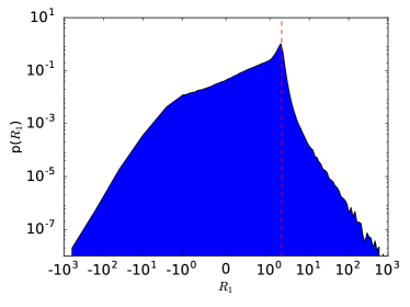
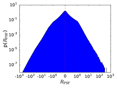
Figure 1.— Left: Normalized distribution of metacalibration shear responsivities from regaussianization, on the Control-Ground-Constant branch of the GREAT3 simulations. Right: Distribution of metacalibration PSF ellipticity responsivities from regaussianization, on the Control-Ground-Constant branch of the GREAT3 simulations. A vertical red dashed line is drawn for reference at the expected responsivity for perfectly round objects, $R=2$, in the left panel.

3.2. Shear Estimation Algorithms

Since the metacalibration method can in principle be used to calibrate shears from any shear estimation algorithm derived using an average of per-object shapes, we chose three easily available shear estimation methods, all of which are implemented in GalSim. Two of these methods are traditional shear estimation methods that have somewhat different assumptions but are both based on object moments. One method is not a standard shear estimation method at all: we use linear combinations of the directly observed second moments without any correction for the PSF. In principle, the information about how those respond to shear should be determined by metacalibration to correctly infer the shear. The difference in this case is that instead of providing a small correction to the outputs of a PSF correction method, we rely on metacalibration to do the entirety of the PSF correction, which is a very stringent test that may at least partially violate some of the assumptions about the ensemble average of the measured quantities having a linear response to shear. The three methods are described below.

3.2.1 Regaussianization

Re-Gaussianization (Hirata & Seljak 2003) is a PSF correction method based on the use of the moments of the image and of the PSF to correct for the effects of the PSF on the galaxy shapes. It includes corrections for the non-Gaussianity of the galaxy profile (Bernstein & Jarvis 2002; Hirata & Seljak 2003) and of the PSF (to first order in the PSF non-Gaussianity). The performance of this algorithm has been extensively studied in real data and simulations (e.g., Mandelbaum et al. 2005, 2012, 2013, 2015).

The outputs of the re-Gaussianization algorithm are PSF-corrected “distortions”, which for an object with purely elliptical isophotes with minor-to-major axis ratio $q$ and position angle $\theta$ with respect to the $x$ axis in pixel coordinates are defined as

$$(e_{1},e_{2})=\frac{1-q^{2}}{1+q^{2}}\left(\cos{2\theta},\sin{2\theta}\right).$$ (9)

As discussed in Bernstein & Jarvis (2002), the response of a distribution of galaxies with some intrinsic distribution of distortions $p(e)$ to a shear depends on the $p(e)$ itself. Conceptually, we can think of an ensemble shear estimator using re-Gaussianization outputs as

$$\hat{g}_{j}=\frac{\langle e_{j}\rangle}{\mathrm{d}\langle e_{j}\rangle/\mathrm{d}g_{j}}$$ (10)

where the denominator gives the response of the ensemble average distortion to a shear (often called the responsivity). Estimators of this shear responsivity use the observed galaxy $p(e)$ and its moments, and for typical $p(e)$, the denominator is around $1.7$–$1.8\approx 2(1-e_{\text{RMS}}^{2})$ in terms of the per-component RMS distortion. As this implementation was meant to be a simple and fast example, its intrinsic calibration correction is a simple one that does not include all known systematics.

3.2.2 KSB

The KSB method (Kaiser et al. 1995) parametrises galaxies and stars according to their weighted quadrupole moments. The main assumption of the KSB method is that the PSF can be described as a small but highly anisotropic distortion convolved with a large circularly symmetric function. With that assumption, the shear can be recovered to first-order from the observed ellipticity of each galaxy via

$$g=P_{g}^{-1}\left(e^{\rm obs}-\frac{P^{\rm sm}}{P^{\rm sm*}}e^{*}\right),$$ (11)

where asterisks indicate quantities that should be measured from the PSF model at that galaxy position, $P^{\rm sm}$ is the smear polarisability (see Heymans et al. 2006 for definitions) and $P_{g}$ is the correction to the shear polarisability that includes the smearing with the isotropic component of the PSF. The ellipticities are constructed from weighted quadrupole moments, and the other quantities involve higher order moments. A circular Gaussian weight of scale length $r_{g}$ is used, where $r_{g}$ is galaxy size, as determined by the second moment of the surface-brightness profile.

The KSB method returns a per-object estimate of the shears $(\hat{g}_{1},\hat{g}_{2})$. We can use metacalibration to remove multiplicative and additive biases that come from averaging the per-object KSB shear estimates.

3.2.3 Linear Moments

As mentioned previously, the third method we use does not involve PSF-corrected galaxy shapes. Instead, we use linear combinations of the second moments of galaxy images. The motivation behind this choice is as follows. One way to estimate the distortion $(e_{1},e_{2})$ is via combinations of the second moments of the light profile,

$$\langle x_{i}\rangle=\frac{\int x_{i}w({\mathbf{x}})I({\mathbf{x}})\mathrm{d}^{2}{\mathbf{x}}}{\int w({\mathbf{x}})I({\mathbf{x}})\mathrm{d}^{2}{\mathbf{x}}}$$ (12)

for $i=1,2$,

$$M_{ij}=\frac{\int(x_{i}-\langle x_{i}\rangle)(x_{j}-\langle x_{j}\rangle)w({\mathbf{x}})I({\mathbf{x}})\mathrm{d}^{2}{\mathbf{x}}}{\int w({\mathbf{x}})I({\mathbf{x}})\mathrm{d}^{2}{\mathbf{x}}}$$ (13)

for $i,j=1,2$, and finally

$$e_{1}=\frac{M_{11}-M_{22}}{M_{11}+M_{22}},\qquad e_{2}=\frac{2M_{12}}{M_{11}+M_{22}}.$$ (14)

One source of noise (and noise bias) in traditional moments-based methods is the division of two noisy quantities in Eq. 14, typically followed by further division by other noisy quantities to remove the dilution of the galaxy shape by the PSF. Thus, as a final example of a statistic that we will attempt to use as a calibrated shear estimator with metacalibration, we define the following linear combinations of moments:

$$\hat{M}_{i}=(M_{11}-M_{22},2M_{12}).$$ (15)

Clearly these moments are sensitive to a number of nuisance quantities, like the galaxy flux and size, and the PSF size and shape. In principle, metacalibration should be able to nonetheless determine the response of this statistic to shear, $\mathrm{d}\hat{M}_{i}/\mathrm{d}g$, and produce a reliable shear estimate from the ensemble-averaged $\hat{M}_{i}$ values, provided that the linear model for the signal and dominant sources of systematic error is correct. This is a quite stringent test of the metacalibration method, as it is unclear whether that purely linear model will be valid in this case.

3.3. Per-Object Responsivity

Shape measurements on the set of modified images can be used to derive noisy shear and PSF responsivities for individual galaxies. In the case where the measured ellipticity is thought to depend linearly on the lensing shear and the PSF ellipticity, the shapes measured from the sheared, reconvolved images with positive and negative applied shears, $\mathbf{e}_{+}$ and $\mathbf{e}_{-}$, can be used for a straightforward finite-difference estimate of the per-object shear response

$$R =\frac{\partial\mathbf{e}}{\partial\mathbf{g}}$$ (16)

$$=\frac{\mathbf{e}_{+}-\mathbf{e}_{-}}{2\Delta\mathbf{g}}$$ (17)

Additive biases introduced by the shape measurement can be extracted from the sum of these two quantities

$$\mathbf{c}=\frac{\mathbf{e}_{+}+\mathbf{e}_{-}}{2}-\mathbf{e},$$ (18)

where the final $\mathbf{e}$ on the right-hand side is the ellipticity measured using the reconvolved PSF $\Gamma$, not that measured from the unmodified original image.

If the shape measurement algorithm does not perfectly remove PSF ellipticity, then the shapes measured from shearing the PSF ($\mathbf{e}_{+,\rm PSF}$ and $\mathbf{e}_{-,\rm PSF}$) permit calculation of at least the linear-order residual PSF ellipticity biases:

$$R_{\rm PSF}=\frac{\mathbf{e}_{+,\rm PSF}-\mathbf{e}_{-,\rm PSF}}{2\Delta\mathbf{g}}.$$ (19)

The result of this process is a catalog of per-object shear and PSF responsivities every galaxy. A histogram of these quantities for one of the measurement algorithms examined in this paper is shown in figure 1.

Accurate calibration depends on characterising the ensemble response, however, not the per-object responses. We argue that the power-law wings of the distribution make estimation of the ensemble response by simple averaging problematic, and describe next a general scheme for regularizing the ensemble response estimation. These wings are a consequence of the fact that the regaussianization shapes are themselves ratios of noisy quantities; other methods with more compact support may not require this sort of regularization scheme.

3.4. Ensemble Responsivity

We test the metacalibration procedure on two different shear estimation methods – regaussianization and KSB – each of which is known to have calibration biases that depend on the $S/N$, galaxy size and morphology, and so on. For both methods, we use the entire ensemble of measured shapes to build a model of the unlensed shape distribution, $p_{0}(\mathbf{e})$. There is no guarantee that the average shear (or PSF ellipticity) over the ensemble is actually small enough that the effective mean ellipticity is zero, however. Before proceeding with the inference, we subtract from each galaxy the expected contribution from the PSF for its field, $R_{\rm PSF}e_{\rm PSF}$. We then symmetrize the resulting distribution by averaging it with its reflection about $\mathbf{e}=0$ (note that the resulting model for the null shape distribution will be somewhat broader than the true distribution of ellipticities at zero shear). The newly symmetrized model unlensed distribution is $p_{0,\rm sym}$. We perform the same PSF subtraction from the measured catalog prior to performing inference in the procedure described below.

If the measured shape distribution $n(\mathbf{e}_{\rm meas})$ is linear in the shear, then we can write

$$\frac{n(\mathbf{e}_{\rm meas})}{N_{tot}}=p_{0,\rm sym}(\mathbf{e})+\mathbf{g}\cdot\partial_{g}p_{0,\rm sym}(\mathbf{e})$$ (20)

It will be convenient to discretize this distribution into a histogram. If the probability of a galaxy ending up in the $i^{\rm th}$ shape histogram bin is $q_{i}$, and each galaxy’s shape can be considered an independent draw from some underlying distribution, then the likelihood function for an observed histogram is the multinomial likelihood

$$p(\left\{N_{i}\right\}|\left\{q_{i}\right\})=\frac{N_{\rm tot}!}{\prod\limits_{i}(N_{i}!)}\prod\limits_{j}q_{j}^{N_{j}}$$ (21)

where $N_{\rm tot}=\sum\limits_{i}N_{i}$ is the total number of samples in the histogram. The covariance matrix for the bin amplitudes of this histogram is

$${\rm cov}(N_{i},N_{j})=C_{ij}=\begin{cases}q_{i}(1-q_{i})N_{\rm tot},&i=j\\ -q_{i}q_{j}N_{\rm tot},&i\neq j.\end{cases}$$ (22)

To make the notation for what follows less cumbersome, let the normalized histogram be $h_{i}=N_{i}/N_{\rm tot}$, and its first derivative with respect to the shear be $\mathbf{\Delta}_{h}=\partial_{g}\mathbf{h}_{\rm fid}$.

Given a measured shape histogram with some unknown shear and a fiducial, unlensed shape histogram, the (component-wise) minimum-variance estimator for $g$ is

$$\hat{g}=\frac{\mathbf{\Delta}_{h}^{T}C^{-1}\left(\mathbf{h}_{\rm meas}-\mathbf{h}_{\rm fid}\right)}{\mathbf{\Delta}_{h}^{T}C^{-1}\mathbf{\Delta}_{h}},$$ (23)

with variance

$$\sigma^{2}_{\hat{g}}=\frac{1}{\mathbf{\Delta}_{h}^{T}C^{-1}\mathbf{\Delta}_{h}}$$ (24)

This method for shear inference has as its tunable parameter only the histogram binning scheme. Once we have chosen a suitable scheme, we then bin the prior into equal-number bins and calculate its shear derivative by adding a small shear $\mathbf{g}$ using the per-object responses, then rebinning. This provides the inputs for the per-field shear estimation. To carry out the per-field shear estimation, we calculate a shape histogram with these bins for each separate field, and evaluate equations 23 and 24 using the globally-derived $\mathbf{\Delta}_{h}^{T}$.

3.5. Validating the Shear Inference

If we have a poor model for the unlensed histogram, $h_{\rm fid}$, then the results for shear inference will be biased. Once we have derived a mean shear for each field, we can quantify the degree to which the shape histogram resembles our model of the unlensed prior distribution.

To do this, we subtract from each galaxy in each field the product of its individual responsivity and the estimated shear (the PSF contribution having already been removed, as above). We then define the distance between each field and the unlensed prior using equation 21, taking the probabilities $q_{i}$ from the unlensed model and the histogram amplitudes from the current field, after correcting for the estimated shear. If the shear response measured for the unlensed prior is correct, then the performance of the estimator will depend only on the similarity of the model to the measurement field. The likelihood can then be used as an objective criterion for the quality of the inference.

In practice, we only apply a cut on the likelihood in cases where we have an a priori reason to believe that the prior constructed as we describe above will not be an adequate description of all of the simulation fields. In our tests below, we apply this cut in simulation branches where there is large expected variation in the PSF properties. In these cases, we exclude from our analysis those fields with the $10\%$ worst log-likelihood cuts.

We can also devise a simple test for the linearity (in the shear) of the ensemble estimator. The estimator we use to infer the shear response relies on two-sided finite-difference numerical derivatives, but it is also possible to get a noisier measure the nonlinear ensemble response by testing for consistency between the forward- and backwards finite-difference estimates for the ensemble response. We quantify this with the parameter $\eta_{\rm nl}$, defined as

$$1+\eta_{nl}=\frac{\Delta_{h+}^{T}C^{-1}\Delta_{h-}}{\Delta_{h}^{T}C^{-1}\Delta_{h}}$$ (25)

where the $+$ and $-$ subscripts refer to the forward- and backwards finite difference histogram derivative estimates.

3.6. Relationship to previous implementations

As shown in the GREAT3 results paper (Mandelbaum et al. 2015), an early version of metacalibration was used in the GREAT3 challenge. That implementation differs from the one presented here and released publicly in association with this paper in two important ways. First, the model for systematics was simpler than the one presented below; it neglected additive systematics entirely, focusing exclusively on multiplicative systematics. Second, the method for inferring shears from an ensemble of objects was entirely different. These differences are of sufficient importance that the GREAT3 results (especially the ones for additive systematics) are not relevant to the implementation described here.

4. Testing Framework

We test the performance of our algorithm on simulated image sets. Our baseline simulations are drawn from the GREAT3 simulation suite. We run additional simulations in order to distinguish between potential biases arising separately from the three steps in our inference framework.

4.1. Simulated Images

We use the GREAT3 simulation framework as the source of simulated images that we use for testing purposes. For more detail about that simulation framework, see the GREAT3 handbook (Mandelbaum et al. 2014) and results paper (Mandelbaum et al. 2015), or the publicly available software.

In brief, we use simulated “branches” containing 200 “subfields”. Each subfield contains $10^{4}$ galaxies placed on a $100\times 100$ grid; the galaxies in a given subfield all have the same (unknown) shear and the same known PSF. The galaxy population within a subfield follows a distribution of signal-to-noise ratio, size, ellipticity, and morphology based on that in the Hubble Space Telescope (HST) COSMOS survey (Koekemoer et al. 2007; Scoville et al. 2007b, a), roughly approximating a galaxy sample with a depth of $I<25$. To ensure that most methods will be able to measure all galaxies, an effective signal-to-noise cut of $\gtrsim 12$ and a minimal resolution cut was imposed (resulting in different sets of galaxies in subfields that have different-sized PSFs). 90^∘ rotated pairs of galaxies were included, to cancel out shape noise (Massey et al. 2007a). The PSF in the simulations comes from the combination of an optics model from a ground-based telescope, along with a Kolmogorov PSF with a typical ellipticity variance. Thus, the galaxy and PSF properties are non-trivially complicated. The noise is stationary Gaussian noise. The ultimate goal is to estimate the average shear in each subfield in an unbiased way, without any multiplicative bias or correlations with the per-subfield PSF ellipticity.

We consider two sets of galaxy populations. One comes directly from HST images, and includes a process to remove the HST PSF before shearing (both operations being carried out in Fourier space) and convolving with the final target PSF (Mandelbaum et al. 2012). The other galaxy population consists of simple parametric representations of those HST images. These populations have the same effective distributions of size, ellipticity, and so on, but one includes realistic galaxy morphology while the other only includes such realism as can be captured by the sum of two Sérsic profiles. In the language of GREAT3, we use simulations corresponding to control-ground-constant (describing the parametric galaxy sample, ground-based simulated data, with a constant per-subfield shear) and real$\_$galaxy-ground-constant (the realistic galaxy sample), denoted CGC and RGC.

4.2. Simulation Branches

The simplest of our simulation tests was performed on a newly-generated set of simulations that is closely analogous to the GREAT3 CGC branch (parametric galaxy profiles), but with one modification to avoid a problem raised in the results paper (Mandelbaum et al. 2015). There, it was noted that the CGC branch has a small fraction of outlier fields related to unusually large optical PSF aberrations, specifically defocus and trefoil. Thus, our first simulated dataset is designed exactly like CGC but with all aberrations in the optical PSF set to zero, to ensure reasonable consistency of data quality. Note that the atmospheric PSF is still drawn from a distribution of seeing values for each subfield. For this branch, it is not necessary to use a likelihood cut to remove fields with aberrant PSF behavior in defining the null ellipticity distribution, and so we include all branches in our analysis. In the accompanying figures and table, this branch is denoted by “CGC-noaber-regauss.”

The next branch we analyze is similar to the previous one, but with realistic galaxies. This lets us separate the effects of realistic galaxy morphology from the problems inherent in correcting a complex PSF. Just as with the previous branch, is not necessary to use a likelihood cut to remove fields with aberrant PSF behavior in defining the null ellipticity distribution, and so we include all the generated fields in our analysis. The results from this branch are labelled “RGC-noaber-regauss.”

We use the GREAT3 CGC simulation branch as a baseline, and report the performance of metacalibration on this branch for all three of our chosen shape measurement algorithms; our results here are denoted in the accompanying figures and tables with the labels “CGC-regauss”, “CGC-moments”, and “CGC-ksb”, as appropriate. Tests on this branch allow straightforward comparison between the performance of our chosen procedure and the variety of other algorithms tested in the GREAT3 challenge.

We next report results for the GREAT3 RGC branch (“RGC-regauss”), incorporating more realistic galaxy morphologies along with the aberrant PSFs introduced in the CGC branch.

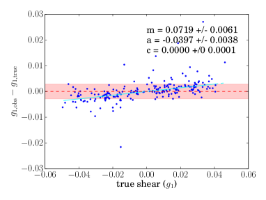
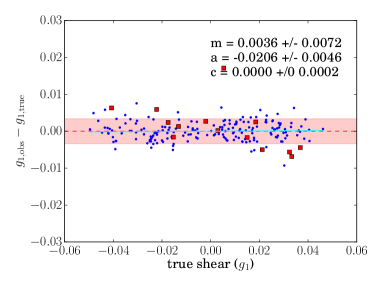
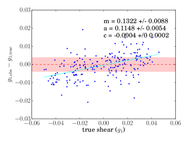
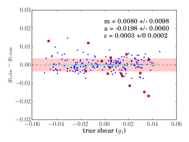
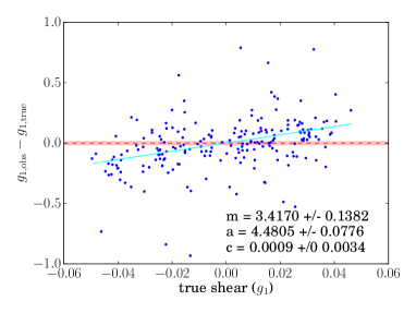
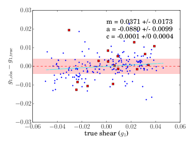
Figure 2.— Shear calibration bias $m_{1}$ before (left) and after right metacalibration for the regaussianization (top), KSB (middle), and Linear Moments (bottom) algorithms on the CGC branch. The shaded region covers the same vertical range in each panel. Points excluded by the log-likelihood cut are marked with red squares.

One issue of concern is how to understand outlier fields. In GREAT3, there was a concern that some outliers were due to failure of our model for interpreting the per-object shapes in fields that had large aberrations. As a way to understand this, we generated a version of RGC that had quite large aberrations that were identical in each field: specifically defocus of $0.5$ waves and one component of trefoil of $0.1$ wave. An example of a PSF in one subfield is shown in Fig. 7; they do not all look identical, since the atmospheric component was still allowed to vary stochastically according to a distribution of seeing FWHM. This removes the difficulties in building a null ellipticity distribution, isolating the impact of a complex PSF. The results from this simulation are labelled “RGC-FixedAber-regauss”.

Finally, we investigate the effects of increasing the noise in the images. We re-run the “CGC-regauss” analysis five times, increasing the noise in the initial image each time. The correlated noise produced by the image modification procedure may affect the derived calibration, and we expect this number of realizations to demonstrate whether correlated noise biases is consistent with the expected signal-to-noise scaling.

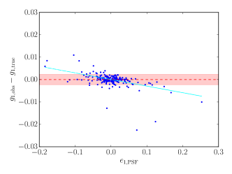
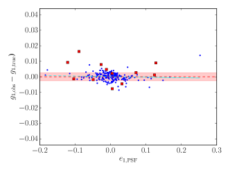
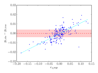
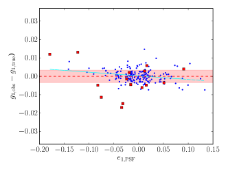
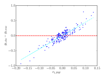
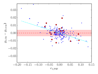
Figure 3.— Effects of the metacalibration algorithm applied to PSF correction. Left panels show the relationship between measured shear and PSF ellipticity before correction, and right panels show the same trends afterwards. Note that the shaded horizontal band covers the same vertical range in each panel. Points rejected by our likelihood cut are shown with red boxes.
Simulation branch/algorithm pairs shown in order from top to bottom are RGC-regauss, CGC-KSB, and CGC-moments. The combination of the metacalibration algorithm with our maximum-likelihood averaging procedure makes accurate corrections when the PSF ellipticities are small or comparable to the magnitude of the shear signal. It is clear that a large fraction of the trend remaining after correction is driven by remaining unmasked high-PSF-ellipticity outlier fields. While these were not rejected by our likelihood criterion, they would typically not pass the image quality requirements in a realistic experiment.

5. Results

Metacalibration reduces the shear calibration biases in every branch that we have tested in, for all methods, and nearly in all cases to a level that is consistent with zero within the errors. In the one branch (CGC-Moments) where it does not eliminate multiplicative biases for both shear components within our ability to measure them, it reduces $m$ by a factor of eighty. Our objective criterion for the quality of per-field mean shear inference generally succeeds in flagging problem fields, and (as is visible in figure 2), the metacalibrated shears tend to be less noisy than the un-metacalibrated shears.

Our PSF detrending algorithm is less successful, probably for reasons we discuss in section 6. Even here, most fields see a significant reduction in the impact of the PSF anisotropy on the inferred shears.

The remainder of section draws conclusions about the performance of the metacalibration algorithm by comparing the results across simulation branches. We discuss the impact of realistic galaxy morphologies, correlated noise, a heterogeneous PSF, and shape measurement algorithms.

The additive and multiplicative calibration biases for each simulation branch, with and without metacalibration, are reported in full in Table 1. Before/after trends for the multiplicative calibration biases and the trends with PSF ellipticity are shown in figures 2 and 3, respectively. Visualizations of the overall impact of metacalibration and PSF ellipticity detrending on the ensemble-average quantities in each branch are provided in Figures 5 and 6.

5.1. Galaxy Morphology

We can compare the performance of the metacalibration algorithm on model and realistic galaxy morphologies in two cases (RGC-regauss vs. CGC-regauss, and RGC-noaber-regauss vs. CGC-noaber-regauss). In neither case does the introduction of realistic morphology have any impact on the multiplicative shear calibration biases: metacalibrating both pairs of branches results in multiplicative biases that are consistent with zero. The most notable difference between the model and real morphologies is apparent in the PSF trends. Our perturbative PSF detrending scheme reduces the residual additive bias in most cases, but it does not completely correct the model morphologies, whereas there is no evidence of any residual PSF effects in any of the realistic morphology branches. This should not surprise us: we have chosen to perturb and detrend the linear effects of PSF ellipticity, but other PSF properties may be more significant and hence our model is not a complete description of additive systematics. The coupling between PSF morphology and inferred shear will in general depend on the details of both, as well as the galaxy morphology and measurement algorithm. We defer further development of methods to select appropriate control variables for PSF detrending to future work.

5.2. Correlated Noise

The image reconvolution procedure described in section 2.1 also modifies the noise field in the original image: the isotropic white noise typical of real images will be transformed in the counterfactual images into a correlated noise field with preferred direction and scale.

This effect was first documented in the context of shear measurement in the work described in Sheldon & Huff (2017) in simulations conducted at much lower signal-to-noise ratios than those of the Great3 challenge. A fuller exploration of the impact of correlated noise on metacalibration, along with a comprehensive mitigation strategy, is presented in that work.

We investigate the impact of this noise by successively adding noise to the CGC images and re-running the metacalibration and shear estimation algorithms. In the process we gradually increase the noise relative to its initial level by up to a factor of $3.5$.

The additive biases resulting from varying the noise level are shown in Figure 4. For the typical signal-to-noise ratios seen in the GREAT3 simulations, biases resulting from correlated noise appear to scale roughly as the variance of the initial noise field. We note that these effects do not become significant until the overall signal-to-noise ratio has been reduced by a factor of two compared to the fiducial GREAT3 values.

The case of the factor of two increase is denoted “CGC-regauss-noisy” in Table 1 and Figures 5 and 6.

5.3. Heterogeneous PSF

Large variations in the PSF properties can impact our measurement algorithm via two channels: first, a heterogeneous PSF can result in individual fields deviating from the zero-shear distribution constructed from the ensemble of measured shapes, potentially biasing the histogram estimator; and second (as discussed above) via the usual mechanism of incomplete PSF correction and detrending.

Eliminating outlier fields in those branches with large variations in the PSF via the rejection mechanism described in section 3.5 tends to significantly improve the calibration bias after metacalibration. The rejected fields (red squares in Figure 3) tend to have substantially larger residual shear calibration biases than the mean field in each branch, and without the outlier rejection, we see few-percent level calibration biases in each of these branches. With the likelihood-based rejection mechanism in place, the multiplicative and additive biases in the CGC and RGC-regauss branches are consistent with those in the CGC-noaber and RGC-noaber branches. It should be noted that we arrived at the $10\%$ cut by choosing a level that typically eliminated outliers from the compact core of the distribution of per-field likelihoods. There are certainly more objective ways to choose this cut – one can eliminate fields that are much lower than the values generated by sampling from equation (21), for instance – but we defer calibration of the outlier-rejection technique to future work.

Finally, we compare the performance of metacalibration in the RGC-noaber, and RGC-FixedAber branches. These branches have a relatively homogenous PSF, differing only in the complexity of the PSF morphology (see Figure  7). We see only marginal evidence ($\sim 1.5\sigma$) for residual calibration biases in this case (though this is the only significant bias seen among the six regauss fields we report on, so a single $\sim 1\sigma$ detection is to be expected even in the absence of any real calibration biases). It is also notable that the RGC-FixedAber branch sees no significant trend between PSF anisotropy and inferred shear.

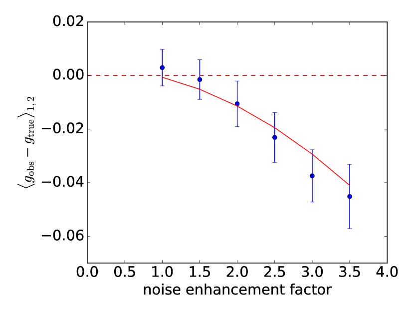
Figure 4.— Effects of introducting additional noise. Points with errors correspond to additive shear bias in the control-ground-constant branch when additional noise is added. The noise enhancement factor corresponds to the factor by which the noise in each galaxy image is increased relative to the fiducial GREAT3 simulations. The solid red line shows the expected power-law scaling resulting from correlated noise bias, with a normalization fixed to the measured additive biases.

Given these results, it would seem that the primary channel through which a heterogeneous PSF impacts our shear inference is via the first channel; the ensemble response of those fields with outlier PSF properties is sufficiently different from that estimated from the global null ellipticity distribution that identification of these fields is essential.

5.4. Shape Measurement Algorithms

We investigate the effects of the shape measurement algorithm by comparing the performance of the regauss, KSB, and linear moments measurement algorithms on the CGC simulation branch. We see large improvements in performance for each method after using metacalibration. There is weak evidence for residual KSB calibration biases, and strong evidence for residual biases in the linear moments. In the latter case, however, the improvement relative to the un-metacalibrated case is large: the multiplicative and additive biases are reduced by factors of $80$ and $51$, respectively, resulting in performance for metacalibrated linear moments that is quantitatively superior to that of the un-metacalibrated KSB. This is remarkable given that simple linear moments involve no PSF correction, leaving the entirety of the PSF correction process to metacalibration.

One potential reason for the difference in performance for different shape measurement methods is the linearity of the ensemble estimates in the resulting shear. We find values for $\eta_{nl}$ of $-0.0034\pm 0.0004$, $-0.024\pm 0.002$, and $-0.0037\pm 0.0004$, for the regauss, KSB, and linear moments algorithms, respectively (where the errors are bootstrap estimates). The quadratic correction to the shear response is much larger for KSB than for the other methods, suggesting that any problems with the KSB shapes may arise from its more nonlinear shear response (see Viola et al. 2011 for a detailed investigation of this issue).

Another potential driver of residual additive systematics is incomplete PSF detrending. The reasons for this are discussed in the previous section. The linear moments see significant PSF residuals, and Figure 3 suggests that these are primarily driven by the fields with large PSF ellipticities.

The $\eta_{nl}$ values and the residual additive and multiplicative biases for these methods suggest that the small residual calibration bias in KSB is driven by the nonlinear response of that shape measurement algorithm, while the residual linear moments calibration bias is primarily driven by imperfect PSF correction.

branch algorithm $m_{1}\times 1000$ $m_{2}\times 1000$ $a_{1}\times 1000$ $a_{2}\times 1000$ $c_{1}\times 1000$ $c_{2}\times 1000$ CGC regauss (MC) $3.6\pm 7.2$ $2.3\pm 6.4$ $-20.6\pm 4.6$ $-19.4\pm 3.6$ $0.0\pm.2$ $0.1\pm 0.2$ CGC regauss $71.9\pm 6.1$ $65.5\pm 4.9$ $-39.7\pm 3.8$ $-43.9\pm 2.9$ $0.0\pm 0.1$ $0.0\pm 0.1$ CGC regauss-noisy (MC) $-15.0\pm 8.9$ $3.7\pm 7.9$ $-24.5\pm 5.7$ $-19.7\pm 4.5$ $-0.1\pm 0.2$ $-0.1\pm 0.2$ CGC regauss-noisy $117.2\pm 7.7$ $105.2\pm 6.6$ $40.2\pm 4.9$ $-48.4\pm 4.1$ $0.2\pm 0.2$ $-0.1\pm 0.2$ CGC ksb (MC) $8.0\pm 9.8$ $-17.0\pm 8.7$ $-19.8\pm 6.0$ $-9.2\pm 5.0$ $0.3\pm 0.2$ $-0.2\pm 0.2$ CGC ksb $132.2\pm 8.8$ $145.5\pm 10.4$ $114.8\pm 5.4$ $109.6\pm 6.1$ $-0.4\pm 0.2$ $0.0\pm.3$ CGC moments (MC) $37.1\pm 17.3$ $45.9\pm 18.4$ $-88.0\pm 9.9$ $-87.7\pm 9.5$ $0.1\pm 0.4$ $-0.2\pm 0.5$ CGC moments $3417.0\pm 138.2$ $3223.8\pm 173.1$ $4480.5\pm 77.6$ $4604.4\pm 88.8$ $0.9\pm 3.4$ $-0.8\pm 4.6$ RGC regauss (MC) $-5.3\pm 7.8$ $6.1\pm 6.6$ $3.6\pm 4.0$ $-3.1\pm 3.7$ $0.1\pm 0.2$ $0.1\pm 0.2$ RGC regauss $30.4\pm 5.2$ $24.9\pm 5.0$ $-29.5\pm 2.8$ $-18.6\pm 2.8$ $0.0\pm 0.1$ $0.2\pm 0.1$ CGC-Noaber regauss (MC) $7.4\pm 6.9$ $6.1\pm 6.9$ $-33.9\pm 12.7$ $-23.7\pm 11.2$ $-0.1\pm 0.2$ $0.1\pm 0.2$ CGC-Noaber regauss $40.7\pm 2.9$ $43.9\pm 2.9$ $-27.4\pm 5.2$ $-26.5\pm 5.0$ $0.1\pm 0.1$ $-0.1\pm 0.1$ RGC-Noaber regauss (MC) $-1.3\pm 5.9$ $4.5\pm 6.4$ $-11.5\pm 11.4$ $-0.8\pm 12.2$ $0.0\pm 0.2$ $-0.1\pm 0.2$ RGC-Noaber regauss $16.4\pm 3.0$ $17.4\pm 3.4$ $2.2\pm 5.8$ $2.5\pm 6.4$ $0.2\pm 0.1$ $0.0\pm 0.1$ RGC-FixedAber regauss (MC) $-11.6\pm 8.9$ $-14.2\pm 7.5$ $17.4\pm 22.6$ $18.3\pm 18.6$ $0.2\pm 0.2$ $-0.2\pm 0.2$ RGC-FixedAber regauss $61.6\pm 6.6$ $63.7\pm 5.2$ $-30.0\pm 12.1$ $-32.3\pm 13.5$ $0.3\pm 0.2$ $0.0\pm 0.1$

Table 1Shear and PSF calibration bias parameters from each of the branches considered. Rows with metacalibrated parameters are shown above their un-calibrated counterparts.

6. Applicability to real data

Several implementation issues need to be solved before this method can be deployed on real survey data. We have made no attempt to deal with the effects of masked pixels or blending, and while it seems clear that our proposed algorithm has the potential to deal with selection biases, we have not demonstrated that capability here. We have also demonstrated the presence of a calibration bias which scales with the variance of the pixel noise, which may be a result of the correlations imposed on the noise field during the construction of the counterfactual image.

In this work, we have attempted to remove PSF systematics by measuring the response of the shape measure to PSF ellipticity. There is no guarantee, however, that the PSF ellipticity is the correct parameter to use for this detrending. In a realistic measurement, it would be best to first determine which modes of PSF variation are most likely to impact the chosen shape measure, and then use the image modification and detrending technique described here to remove those effects in the data.

Finally, our shear inference procedure is designed to extract the mean shear from a constant-shear field. While this procedure may be applicable to galaxy-galaxy lensing (i.e., projecting the shapes onto the tangent to the appropriate lens), it is not suitable for measurements like cosmic shear that typically rely on second or higher moments of the shear field. While a similar histogram estimation procedure could be implemented to model the responsivity of the distribution of ellipticity products (as would be needed for two-point shear correlation functions), we leave design and implementation of this generalization to future work.

At the time of this writing, metacalibration is being actively adapted to realistic measurements in the Dark Energy Survey. Concurrent work (Sheldon & Huff 2017) will demonstrate algorithmic improvements that allow this technique to be used on Dark Energy Survey data with state-of-the-art shear estimation algorithms.

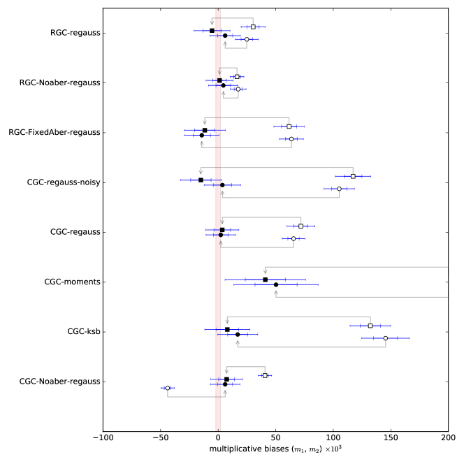
Figure 5.— Calibration bias results. Each row shows muliplicative calibration bias $m_{1}$ (top) and $m_{2}$ (bottom) before and after metacalibration. Pre- and post-correction points are connected by gray arrows: in every case the procedure has reduced or eliminated the amplitude of detectable multiplicative calibration bias.

7. Conclusions

We have proposed and implemented the first method for self-calibration of shear measurements that does not rely on deeper calibration fields or simulations. Our method can be wrapped around any sufficiently well-behaved shape measurement algorithm. We use GREAT3 and related simulations to demonstrate that metacalibration reduces or eliminates shear calibration biases across a variety of galaxy morphologies, PSF properties, and for several otherwise biased shape measurement algorithms. We have argued that our technique works because it takes advantage of the fundamental linearity of astronomical images in the weak lensing shear signal, in combination with the fact that the effects of shear on an image with a known PSF are model-independent.

Those cases we have examined where the initial biases are large or not linear are not completely corrected by our linear detrending scheme, though in every case we have studied the algorithm appears to substantially improve biases resulting from faulty additive PSF correction and multiplicative shear calibration biases. Even the nearly information-free linear moments algorithm appears to be calibrated by our procedure to a level superior to uncorrected KSB, a widely used traditional shear estimation algorithm.

We expect future work to extend this method to deal with the complexities inherent in real data.

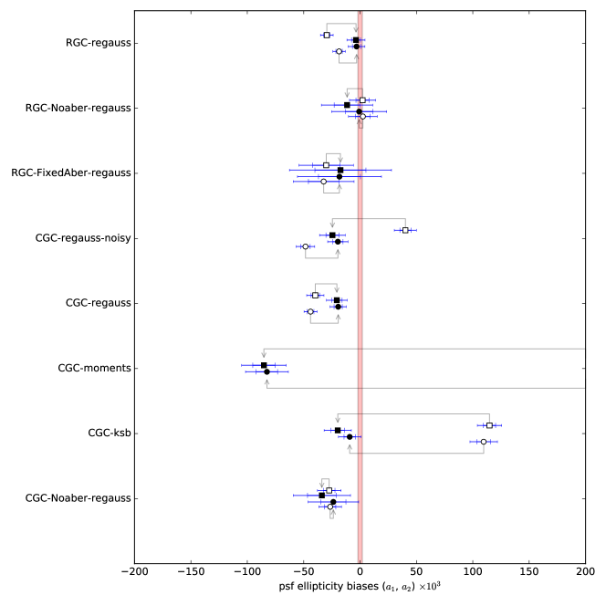
Figure 6.— Additive shear bias results. Each row shows linear coupling between the PSF ellipticity and the measured shape $a_{1}$ (top) and $a_{2}$ (bottom) before and after metacalibration. Pre- and post-correction points are connected by gray arrows: in every case the procedure has reduced or eliminated the amplitude of detectable PSF coupling.

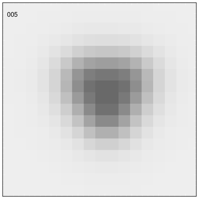
Figure 7.— Example of a PSF in one of the simulations with fixed, large aberrations. The most obvious feature in this case is the trefoil, which gives rise to the triangular shape.

References

- Bartelmann & Schneider (2001) Bartelmann, M. & Schneider, P. 2001, Phys. Rep., 340, 291
- Bergé et al. (2013) Bergé, J., Gamper, L., Réfrégier, A., & Amara, A. 2013, Astronomy and Computing, 1, 23
- Bernstein & Armstrong (2014) Bernstein, G. M. & Armstrong, R. 2014, MNRAS, 438, 1880
- Bernstein & Jarvis (2002) Bernstein, G. M. & Jarvis, M. 2002, AJ, 123, 583
- Bridle et al. (2009) Bridle, S., Shawe-Taylor, J., Amara, A., Applegate, D., Balan, S. T., Berge, J., Bernstein, G., Dahle, H., Erben, T., & et al. 2009, Annals of Applied Statistics, 3, 6
- de Jong et al. (2015) de Jong, J. T. A., Verdoes Kleijn, G. A., Boxhoorn, D. R., Buddelmeijer, H., Capaccioli, M., Getman, F., Grado, A., Helmich, E., Huang, Z., Irisarri, N., Kuijken, K., La Barbera, F., McFarland, J. P., Napolitano, N. R., Radovich, M., Sikkema, G., Valentijn, E. A., Begeman, K. G., Brescia, M., Cavuoti, S., Choi, A., Cordes, O.-M., Covone, G., Dall’Ora, M., Hildebrandt, H., Longo, G., Nakajima, R., Paolillo, M., Puddu, E., Rifatto, A., Tortora, C., van Uitert, E., Buddendiek, A., Harnois-Déraps, J., Erben, T., Eriksen, M. B., Heymans, C., Hoekstra, H., Joachimi, B., Kitching, T. D., Klaes, D., Koopmans, L. V. E., Köhlinger, F., Roy, N., Sifón, C., Schneider, P., Sutherland, W. J., Viola, M., & Vriend, W.-J. 2015, A&A, 582, A62
- Fenech Conti et al. (2016) Fenech Conti, I., Herbonnet, R., Hoekstra, H., Merten, J., Miller, L., & Viola, M. 2016, ArXiv e-prints
- Flaugher (2005) Flaugher, B. 2005, International Journal of Modern Physics A, 20, 3121
- Gruen et al. (2015) Gruen, D., Bernstein, G. M., Jarvis, M., Rowe, B., Vikram, V., Plazas, A. A., & Seitz, S. 2015, Journal of Instrumentation, 10, C05032
- Heymans et al. (2006) Heymans, C., Van Waerbeke, L., Bacon, D., Berge, J., Bernstein, G., Bertin, E., Bridle, S., & et al. 2006, MNRAS, 368, 1323
- Hildebrandt et al. (2016) Hildebrandt, H., Viola, M., Heymans, C., Joudaki, S., Kuijken, K., Blake, C., Erben, T., Joachimi, B., Klaes, D., Miller, L., Morrison, C. B., Nakajima, R., Verdoes Kleijn, G., Amon, A., Choi, A., Covone, G., de Jong, J. T. A., Dvornik, A., Fenech Conti, I., Grado, A., Harnois-Déraps, J., Herbonnet, R., Hoekstra, H., Köhlinger, F., McFarland, J., Mead, A., Merten, J., Napolitano, N., Peacock, J. A., Radovich, M., Schneider, P., Simon, P., Valentijn, E. A., van den Busch, J. L., van Uitert, E., & Van Waerbeke, L. 2016, ArXiv e-prints
- Hirata & Seljak (2003) Hirata, C. & Seljak, U. 2003, MNRAS, 343, 459
- Hoekstra & Jain (2008) Hoekstra, H. & Jain, B. 2008, Annual Review of Nuclear and Particle Science, 58, 99
- Jarvis et al. (2016) Jarvis, M., Sheldon, E., Zuntz, J., Kacprzak, T., Bridle, S. L., Amara, A., Armstrong, R., Becker, M. R., Bernstein, G. M., Bonnett, C., Chang, C., Das, R., Dietrich, J. P., Drlica-Wagner, A., Eifler, T. F., Gangkofner, C., Gruen, D., Hirsch, M., Huff, E. M., Jain, B., Kent, S., Kirk, D., MacCrann, N., Melchior, P., Plazas, A. A., Refregier, A., Rowe, B., Rykoff, E. S., Samuroff, S., Sánchez, C., Suchyta, E., Troxel, M. A., Vikram, V., Abbott, T., Abdalla, F. B., Allam, S., Annis, J., Benoit-Lévy, A., Bertin, E., Brooks, D., Buckley-Geer, E., Burke, D. L., Capozzi, D., Rosell, A. C., Kind, M. C., Carretero, J., Castander, F. J., Clampitt, J., Crocce, M., Cunha, C. E., D’Andrea, C. B., da Costa, L. N., DePoy, D. L., Desai, S., Diehl, H. T., Doel, P., Neto, A. F., Flaugher, B., Fosalba, P., Frieman, J., Gaztanaga, E., Gerdes, D. W., Gruendl, R. A., Gutierrez, G., Honscheid, K., James, D. J., Kuehn, K., Kuropatkin, N., Lahav, O., Li, T. S., Lima, M., March, M., Martini, P., Miquel, R., Mohr, J. J., Neilsen, E., Nord, B., Ogando, R., Reil, K., Romer, A. K., Roodman, A., Sako, M., Sanchez, E., Scarpine, V., Schubnell, M., Sevilla-Noarbe, I., Smith, R. C., Soares-Santos, M., Sobreira, F., Swanson, M. E. C., Tarle, G., Thaler, J., Thomas, D., Walker, A. R., & Wechsler, R. H. 2016, MNRAS
- Kaiser (2000) Kaiser, N. 2000, ApJ, 537, 555
- Kaiser et al. (1995) Kaiser, N., Squires, G., & Broadhurst, T. 1995, ApJ, 449, 460
- Kitching et al. (2013) Kitching, T. D., Rowe, B., Gill, M., Heymans, C., Massey, R., Witherick, D., Courbin, F., Georgatzis, K., Gentile, M., Gruen, D., Kilbinger, M., Li, G. L., Mariglis, A. P., Meylan, G., Storkey, A., & Xin, B. 2013, ApJS, 205, 12
- Koekemoer et al. (2007) Koekemoer, A. M., Aussel, H., Calzetti, D., Capak, P., Giavalisco, M., Kneib, J., Leauthaud, A., Le Fèvre, O., & et al. 2007, ApJS, 172, 196
- Laureijs et al. (2011) Laureijs, R., Amiaux, J., Arduini, S., Auguères, J. ., Brinchmann, J., Cole, R., Cropper, M., Dabin, C., Duvet, L., Ealet, A., & et al. 2011, ArXiv e-prints (1110.3193)
- LSST Science Collaborations & LSST Project (2009) LSST Science Collaborations & LSST Project. 2009, ArXiv e-prints (0912.0201), http://www.lsst.org/lsst/scibook
- Mandelbaum et al. (2012) Mandelbaum, R., Hirata, C. M., Leauthaud, A., Massey, R. J., & Rhodes, J. 2012, MNRAS, 420, 1518
- Mandelbaum et al. (2005) Mandelbaum, R., Hirata, C. M., Seljak, U., Guzik, J., Padmanabhan, N., Blake, C., Blanton, M. R., Lupton, R., & Brinkmann, J. 2005, MNRAS, 361, 1287
- Mandelbaum et al. (2015) Mandelbaum, R., Rowe, B., Armstrong, R., Bard, D., Bertin, E., Bosch, J., Boutigny, D., Courbin, F., Dawson, W. A., Donnarumma, A., Fenech Conti, I., Gavazzi, R., Gentile, M., Gill, M. S. S., Hogg, D. W., Huff, E. M., Jee, M. J., Kacprzak, T., Kilbinger, M., Kuntzer, T., Lang, D., Luo, W., March, M. C., Marshall, P. J., Meyers, J. E., Miller, L., Miyatake, H., Nakajima, R., Ngolé Mboula, F. M., Nurbaeva, G., Okura, Y., Paulin-Henriksson, S., Rhodes, J., Schneider, M. D., Shan, H., Sheldon, E. S., Simet, M., Starck, J.-L., Sureau, F., Tewes, M., Zarb Adami, K., Zhang, J., & Zuntz, J. 2015, MNRAS, 450, 2963
- Mandelbaum et al. (2014) Mandelbaum, R., Rowe, B., Bosch, J., Chang, C., Courbin, F., Gill, M., Jarvis, M., Kannawadi, A., Kacprzak, T., Lackner, C., & et al. 2014, ApJS, 212, 5
- Mandelbaum et al. (2013) Mandelbaum, R., Slosar, A., Baldauf, T., Seljak, U., Hirata, C. M., Nakajima, R., Reyes, R., & Smith, R. E. 2013, MNRAS, 432, 1544
- Massey et al. (2007a) Massey, R., Heymans, C., Bergé, J., Bernstein, G., Bridle, S., Clowe, D., Dahle, H., Ellis, R., & et al. 2007a, MNRAS, 376, 13
- Massey et al. (2010) Massey, R., Kitching, T., & Richard, J. 2010, Reports on Progress in Physics, 73, 086901
- Massey et al. (2007b) Massey, R., Rowe, B., Refregier, A., Bacon, D. J., & Bergé, J. 2007b, MNRAS, 380, 229
- Miyazaki et al. (2012) Miyazaki, S., Komiyama, Y., Nakaya, H., Kamata, Y., Doi, Y., Hamana, T., Karoji, H., Furusawa, H., Kawanomoto, S., Morokuma, T., Ishizuka, Y., Nariai, K., Tanaka, Y., Uraguchi, F., Utsumi, Y., Obuchi, Y., Okura, Y., Oguri, M., Takata, T., Tomono, D., Kurakami, T., Namikawa, K., Usuda, T., Yamanoi, H., Terai, T., Uekiyo, H., Yamada, Y., Koike, M., Aihara, H., Fujimori, Y., Mineo, S., Miyatake, H., Yasuda, N., Nishizawa, J., Saito, T., Tanaka, M., Uchida, T., Katayama, N., Wang, S.-Y., Chen, H.-Y., Lupton, R., Loomis, C., Bickerton, S., Price, P., Gunn, J., Suzuki, H., Miyazaki, Y., Muramatsu, M., Yamamoto, K., Endo, M., Ezaki, Y., Itoh, N., Miwa, Y., Yokota, H., Matsuda, T., Ebinuma, R., & Takeshi, K. 2012, in Proc. SPIE, Vol. 8446, Ground-based and Airborne Instrumentation for Astronomy IV, 84460Z
- Refregier (2003) Refregier, A. 2003, ARA&A, 41, 645
- Rowe et al. (2015) Rowe, B. T. P., Jarvis, M., Mandelbaum, R., Bernstein, G. M., Bosch, J., Simet, M., Meyers, J. E., Kacprzak, T., Nakajima, R., Zuntz, J., Miyatake, H., Dietrich, J. P., Armstrong, R., Melchior, P., & Gill, M. S. S. 2015, Astronomy and Computing, 10, 121
- Schneider (2006) Schneider, P. 2006, in Saas-Fee Advanced Course 33: Gravitational Lensing: Strong, Weak and Micro, ed. G. Meylan, P. Jetzer, P. North, P. Schneider, C. S. Kochanek, & J. Wambsganss, 269–451
- Scoville et al. (2007a) Scoville, N., Abraham, R. G., Aussel, H., Barnes, J. E., Benson, A., Blain, A. W., Calzetti, D., Comastri, A., Capak, P., & et al. 2007a, ApJS, 172, 38
- Scoville et al. (2007b) Scoville, N., Aussel, H., Brusa, M., Capak, P., Carollo, C. M., Elvis, M., Giavalisco, M., Guzzo, L., Hasinger, G., & et al. 2007b, ApJS, 172, 1
- Sheldon & Huff (2017) Sheldon, E. S. & Huff, E. M. 2017, ApJ, submitted
- Spergel et al. (2015) Spergel, D., Gehrels, N., Baltay, C., Bennett, D., Breckinridge, J., Donahue, M., Dressler, A., Gaudi, B. S., Greene, T., Guyon, O., Hirata, C., Kalirai, J., Kasdin, N. J., Macintosh, B., Moos, W., Perlmutter, S., Postman, M., Rauscher, B., Rhodes, J., Wang, Y., Weinberg, D., Benford, D., Hudson, M., Jeong, W.-S., Mellier, Y., Traub, W., Yamada, T., Capak, P., Colbert, J., Masters, D., Penny, M., Savransky, D., Stern, D., Zimmerman, N., Barry, R., Bartusek, L., Carpenter, K., Cheng, E., Content, D., Dekens, F., Demers, R., Grady, K., Jackson, C., Kuan, G., Kruk, J., Melton, M., Nemati, B., Parvin, B., Poberezhskiy, I., Peddie, C., Ruffa, J., Wallace, J. K., Whipple, A., Wollack, E., & Zhao, F. 2015, ArXiv e-prints
- Viola et al. (2011) Viola, M., Melchior, P., & Bartelmann, M. 2011, MNRAS, 410, 2156
- Weinberg et al. (2013) Weinberg, D. H., Mortonson, M. J., Eisenstein, D. J., Hirata, C., Riess, A. G., & Rozo, E. 2013, Phys. Rep., 530, 87
- Zhang & Komatsu (2011) Zhang, J. & Komatsu, E. 2011, MNRAS, 414, 1047