Ferroelectric glass of spheroidal dipoles with impurities: Polar nanoregions,
response to applied electric field, and ergodicity breakdown

Abstract

Using molecular dynamics simulation, we study dipolar glass in crystals composed of slightly spheroidal, polar particles and spherical, apolar impurities between metal walls. We present physical pictures of ferroelectric glass, which have been observed in relaxors, mixed crystals (such as KCN_xKBr_1-x), and polymers. Our systems undergo a diffuse transition in a wide temperature range, where we visualize polar nanoregions (PNRs) surrounded by impurities. In our simulation, the impurities form clusters and their space distribution is heterogeneous. The polarization fluctuations are enhanced at relatively high $T$ depending on the size of the dipole moment. They then form frozen PNRs as $T$ is further lowered into the nonergodic regime. As a result, the dielectric permittivity exhibits the characteristic features of relaxor ferroelectrics. We also examine nonlinear response to cyclic applied electric field and nonergodic response to cyclic temperature changes (ZFC$/$FC), where the polarization and the strain change collectively and heterogeneously. We also study antiferroelectric glass arising from molecular shape asymmetry. We use an Ewald scheme of calculating the dipolar interaction in applied electric field.

I Introduction

Ferroelectric transitions have been attracting much attention in various systems. It is known that they can occur even in simple particle systems. For example, one-component spherical particles with a point dipole undergo a ferroelectric transition in crystal or liquid-crystal phases if the dipole interaction is sufficiently strong Gao ; Wei ; Weis ; Ta ; Tao ; Ayton ; Hent0 ; Hent ; Dij0 ; Groh . Such spherical dipoles form various noncubic crystals in ferroelectric phases Groh ; Dij0 . Ferroelectriciity was also studied in positionally disordered dipolar solidsAyton . Recently, Johnson et al.Johnson0 ; Johnson1 have investigated a ferroelectric transition of spheroidal particles with a dipole moment $\mu_{0}$ parallel to the spheroidal axis. They found that the static dielectric constant increases up to $10^{2}-10^{3}$ with increasing $\mu_{0}$ if the aspect ratio is close to unity. In this paper, we examine ferroelectric transitions in mixtures of slightly spheroidal dipoles and spherical impurities.

In many solids, the polarization is induced by ion displacements within unit cells and the dielectric constant is very large. As a unique aspect, the ferroelectric transitions become diffuse with a sufficient amount of disorderVug ; Bl ; Kob , which take place over a wide temperature range without long-range dipolar order. Notable examples are relaxors Smo ; Klee ; Klee1 ; Bokov3 ; Bokov ; Bl ; Cr ; Cowley ; Samara such as Pb(Mg_1/3Nb_2/3)O₃ (PMN), where the random distribution of Mg²⁺ and Nb⁵⁺ at B sites yields quenched random fields at Pb²⁺ sites Setter ; West . In relaxors, temperature-dependence of the optic index of refraction suggested appearance of mesoscopic polarization heterogeneities Burns , called polar nanoregions (PNRs). They are enhanced at relatively high $T$ as near-critical fluctuations and are frozen at lower $T$. It is widely believed that these PNRs give rise to a broad peak in the dielectric permittivity $\varepsilon^{\prime}$ as a function of $T$ Setter ; Smo ; Klee ; Klee1 ; Bl ; Cr ; Cr1 ; Bokov ; Bokov3 ; Cowley ; Samara ; Ra . They have been detected by neutron and x-ray scattering Wel ; Stock ; Eg ; Shi1 ; Shi2 ; Cowley and visualized by transmission electron microscopy Ban ; Mori ; Uesu and piezoresponse force microscopy Bokov2 ; Bokov4 ; Ann . Strong correlations have also been found between the PNRs and the compositional heterogeneity of the B site cations Wel ; Wel1 ; Ban ; Setter ; Bokov4 ; Mori ; Perrin ; Jin ; i3 ; i6 .

Relaxor behaviors also appear in other disordered dipolar systemsBl ; Kob ; Vug . In particular, orientational glass has long been studied in mixed crystals such as KCN_xKBr_1-x or K_xLi_1-xTaO₃ Vug ; Tou ; Ho1 ; Ho2 ; Loidl3 ; qua ; ori ; Binder ; anti-Loidl ; Yokota ; Mertz ; F3 , where the two mixed components have similar sizes and shapes. Upon cooling below melting, they first form a cubic crystal without long-range orientational order in the plastic crystal phase. At lower $T$, an orientational phase transition occurs, where the crystal structure becomes noncubic. In nondilute mixtures, this transition is diffuse with slow relaxations, where the orientations and the strains are strongly coupled, both exhibiting nanoscale heterogeneitiesqua ; Heuer ; Takae-ori ; EPL . Some polymers also undergo ferroelectric transitions due to alignment of permanent dipoles Bl ; Lov ; Furukawa ; Furu1 . In particular, poly(vinylidene fluoride-trifluoroethylene) copolymersZhang ; Z1 exhibited large electrostriction and relaxor-like polarization responses after electron irradiation (which brings disorder in polymer crystals). We also mention strain glass in shape-memory alloys F5 , where the dipolar interaction does not come into play but a diffuse ferroelastic transition occurs with strain heterogeneities. We now recognize the universal features of glass coupled with a phase transition, where the order parameter fluctuations are frozen at low $T$.

In their molecular dynamics simulation of relaxors, Burton et al.Burton1 ; Burton2 ; Burton3 started with a first-principles Hamiltonian for atomic displacements in perovskite-type crystals. As a compositional distribution, they assumed nanoscale chemically ordered regions embedded in a chemically disordered matrix. On the other hand, we investigate general aspects of ferroelectric glass with a simple molecular model. In electrostatics, we use an Ewald scheme including image dipoles and applied electric field apply ; Klapp , which has been used to study water between electrodesHautman ; Takae1 ; Takae2 . To prepare a mixed crystal, we cool a liquid mixture from high $T$; then, our impurity distribution at low $T$ is naturally formed during crystallization Takae-ori ; EPL .

Our system consists of spheroidal dipoles and spherical apolar particles only. Nevertheless, we can realize enhanced polarization fluctuations forming PNRs and calculate the frequency-dependent dielectric permittivity. We can also calculate the responses to applied electric field and to ZFC$/$FC (zero-field-cooling and field-cooling) temperature changes. In the latter, nonergodicity of glass is demonstrated, so its experiments have been performed in spin glassMydosh ; F0 ; F1 , relaxorsWest ; Uesu ; F4 , orientational glassHo1 ; F3 , relaxor-like polymers Z1 , and strain glassF5 .

The organization of this paper is as follows. In Sec. II, we will explain our theoretical scheme and numerical method. In Sec. III, we will explain a structural phase transition in a one-component system of dipolar spheroids. In Sec. IV, we will examine diffuse ferroelectric transitions with impurities. Furthermore, we will examine responses to cyclic applied field in Sec.V and to cyclic temperature changes in Sec.VI. Additionally, antiferroelectric glass will be briefly discussed In Sec.VII.

II Theoretical background

We treat mixed crystals composed of spheroidal polar particles as the first species and spherical apolar particles (called impurities) as the second species. These particles have no electric charge. As in Fig.1(a), we suppose smooth metal walls at $z=0$ and $H$ to apply electric field to the dipoles. The periodic boundary condition is imposed along the $x$ and $y$ axes with period $L$. Thus, the particles are in a $L\times L\times H$ cell with volume $V=L^{2}H$.

In terms of the impurity concentration $c$, the particle numbers of the two species are written as

$$N_{1}=Vn_{1}=(1-c)N,\quad N_{2}=Vn_{2}=cN,$$ (1)

where the total particle number $N$ is set equal to $8000$. Their positions are written as ${\mbox{\boldmath$r$}}_{i}=(x_{i},y_{i},z_{i})$ ($1\leq i\leq N$). The long axes of the spheroidal particles are denoted by unit vectors ${\mbox{\boldmath$n$}}_{i}=(n_{xi},n_{yi},n_{zi})$ ($1\leq i\leq N_{1}$).

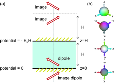
Figure 1: (a) Illustration of geometry. Dipoles are in a cell (green region) and two kinds of image dipoles are outside it. Parallel metallic plates are at $z=0$ and $H$. Electric potential is 0 at $z=0$ and is $-\Delta\Phi=-E_{\rm a}H$ at $z=H$. (b) Color maps of dipole orientation on a sphere surface used in the following figures. Displayed from above are diagonally downward view, diagonally upward view, top view, and bottom view.

II.1 Potential energy

The total potential energy $U$ is expressed as

$$U=U_{\rm LJ}+U_{\rm w}+U_{\rm d}.$$ (2)

Here, $U_{\rm LJ}$ is the sum of modified Lennard-Jones potentials between particles $i\in\alpha$ and $j\in\beta$ ($\alpha,\beta=1,2$),

$$U_{\rm LJ}=2\epsilon\sum_{i\neq j}\bigg{[}(1+A_{ij})\frac{\sigma_{\alpha\beta}^{12}}{r_{ij}^{12}}-\frac{\sigma_{\alpha\beta}^{6}}{r_{ij}^{6}}\bigg{]}.$$ (3)

where $r_{ij}=|{\mbox{\boldmath$r$}}_{i}-{\mbox{\boldmath$r$}}_{j}|$, $\epsilon$ is the characteristic interparticle energy, and $\sigma_{\alpha\beta}=(\sigma_{\alpha}+\sigma_{\beta})/2$ in terms of the particle lengths $\sigma_{1}$ and $\sigma_{2}$. The factor $A_{ij}$ depends on the angles between spheroid directions and ${\mbox{\boldmath$r$}}_{ij}={\mbox{\boldmath$r$}}_{i}-{\mbox{\boldmath$r$}}_{j}$ as EPL ; Takae-ori

$$A_{ij}=\delta_{\alpha 1}{\eta}({\mbox{\boldmath$n$}}_{i}\cdot{\mbox{\boldmath$r$}}_{ij}/r_{ij})^{2}+\delta_{\beta 1}{\eta}({\mbox{\boldmath$n$}}_{j}\cdot{\mbox{\boldmath$r$}}_{ij}/r_{ij})^{2},$$ (4)

where $i\in 1$ in the first term, $j\in 1$ in the second term, and $\eta$ represents the molecular anisotropy. For $\eta>0$, we have $0\leq A_{ij}\leq 2\eta$, which vanishes for ${\mbox{\boldmath$n$}}_{i}\cdot{\mbox{\boldmath$r$}}_{ij}=0$ for $j\in 2$ (and ${\mbox{\boldmath$n$}}_{j}\cdot{\mbox{\boldmath$r$}}_{ij}=0$ for $j\in 1$). We assume a relatively small size difference and mild anisotropy as

$$\sigma_{2}/\sigma_{1}=1.1,\quad\eta=1.2.$$ (5)

Then, at density $0.84\sigma_{1}^{-3}$, our system forms a crystal without phase separation and isotropic-nematic phase transition Latz ; EPL . For larger $\sigma_{2}/\sigma_{1}$ and $\eta$, the latter processes may take place during slow quenching from liquid. Because $U_{\rm LJ}$ is minimized at $r_{ij}=(2+2A_{ij})^{1/6}\sigma_{\alpha\beta}$ for fixed ${\mbox{\boldmath$n$}}_{i}$ and ${\mbox{\boldmath$n$}}_{j}$, we regard the anisotropic particles as spheroids with aspect ratio $(1+2\eta)^{1/6}=1.24$. Notice that our potential is similar to the Gay-Berne potential for rodlike molecules Berne .

The second term $U_{\rm w}$ in Eq.(2) is the sum of strongly repulsive, wall potentials as apply

$$U_{\rm w}=w\sum_{i}[\exp(-z_{i}/\xi_{\rm w})+\exp(-(H-z_{i})/\xi_{\rm w})],$$ (6)

We set $w=e^{40}\epsilon$ and $\xi_{\rm w}=0.01\sigma_{1}$ to make the potentials hardcore-like. Then, the distances between the dipole centers and the walls become longer than $0.4\sigma_{1}$.

II.2 Electrostatic energy and canonical distribution

We assume permanent dipolar moments ${\mbox{\boldmath$\mu$}}_{i}$ along the spheroid direction ${\mbox{\boldmath$n$}}_{i}$ ($1\leq i\leq N_{1}$) written as

$${\mbox{\boldmath$\mu$}}_{i}=(\mu_{xi},\mu_{yi},\mu_{zi})=\mu_{0}{\mbox{\boldmath$n$}}_{i},$$ (7)

where $\mu_{0}$ is a constant dipole moment. There is no induced dipole moment. The electric potential $\Phi({\mbox{\boldmath$r$}})$ can be defined away from the dipole positions ${\mbox{\boldmath$r$}}\neq{\mbox{\boldmath$r$}}_{i}$. We impose the metallic boundary condition at $z=0$ and $H$:

$$\Phi(x,y,0)=0,\quad\Phi(x,y,H)=-\Delta\Phi=-E_{\rm a}H,$$ (8)

where $\Delta\Phi$ is the applied potential difference and $E_{\rm a}=\Delta\Phi/H$ is the applied electric field. In this paper, we perform simulation by controlling $\Delta\Phi$ (or $E_{\rm a}$). In our scheme, $\Delta\Phi$ can be nonstationary.

The boundary condition (8) is realized by the surface charge densities at $z=0$ and $H$ (see Appendix A). As a mathematical convenience, we instead introduce image dipoles outside the cell for each dipole ${\mbox{\boldmath$\mu$}}_{i}$ at ${\mbox{\boldmath$r$}}_{i}=(x_{j},y_{j},z_{j})$ in the cell. As in Fig.1(a), we first consider those at ${\mbox{\boldmath$r$}}_{i}-2Hm_{z}{\mbox{\boldmath$e$}}_{z}$ ($m_{z}=\pm 1,\pm 2,\cdots$) with the same moment ${\mbox{\boldmath$\mu$}}_{i}$, where ${\mbox{\boldmath$e$}}_{z}$ is the unit vector along the $z$ axis. Second, at ${\bar{\mbox{\boldmath$r$}}}_{i}-2Hm_{z}{\mbox{\boldmath$e$}}_{z}$ $(m_{z}=0,\pm 1,\pm 2,\cdots)$, we consider those with the image moment given by

$$\bar{\mbox{\boldmath$\mu$}}_{i}=(-\mu_{xi},-\mu_{yi},\mu_{zi}),$$ (9)

where ${\bar{\mbox{\boldmath$r$}}}_{i}=(x_{i},y_{i},-z_{i})$ is the image position closest to the bottom wall. For ${\mbox{\boldmath$r$}}\neq{\mbox{\boldmath$r$}}_{i}$, the real and image dipoles and the applied field yield the following potential,

$$\Phi({\mbox{\boldmath$r$}}) = \sum_{{\mbox{\boldmath$h$}}}{\sum_{j\in 1}}\bigg{[}{\mbox{\boldmath$g$}}({{\mbox{\boldmath$r$}}-{\mbox{\boldmath$r$}}_{j}+{\mbox{\boldmath$h$}}})\cdot{\mbox{\boldmath$\mu$}}_{j}$$ (10)

$$+{\mbox{\boldmath$g$}}({{\mbox{\boldmath$r$}}-{\bar{\mbox{\boldmath$r$}}}_{j}+{\mbox{\boldmath$h$}}})\cdot{\bar{\mbox{\boldmath$\mu$}}}_{j}\bigg{]}-E_{\rm a}z,$$

where ${\mbox{\boldmath$r$}}\neq{\mbox{\boldmath$r$}}_{i}$, ${\mbox{\boldmath$g$}}({\mbox{\boldmath$r$}})=r^{-3}{\mbox{\boldmath$r$}}$, and ${\mbox{\boldmath$h$}}=(Lm_{x},Lm_{y},2Hm_{z})$ with $m_{x},m_{y}$, and $m_{z}$ being integers. Here, the first term is periodic in three dimensions (3D). Along the $z$ axis the period is $2H$ because of the summation over $m_{z}$ or over the image dipoles. We confirm that the first term in Eq.(10) vanishes at $z=0$ and $H$ with the aid of Eq.(9).

At fixed $E_{\rm a}$, the total electrostatic energy $U_{\rm d}$ in Eq.(2) is now written in terms of ${\mbox{\boldmath$r$}}_{i}$ and ${\mbox{\boldmath$\mu$}}_{i}$ asKlapp ; apply

$$U_{\rm d}=\frac{1}{2}\sum_{{\mbox{\boldmath$h$}}}{\sum_{i\in 1,j\in 1}}^{\prime}{\mbox{\boldmath$\mu$}}_{i}\cdot{\stackrel{{\scriptstyle\leftrightarrow}}{{\mbox{\boldmath$\cal T$}}}}({\mbox{\boldmath$r$}}_{ij}+{\mbox{\boldmath$h$}})\cdot{\mbox{\boldmath$\mu$}}_{j}$$

$$+\frac{1}{2}\sum_{{\mbox{\boldmath$h$}}}{\sum_{i\in 1,j\in 1}}{\mbox{\boldmath$\mu$}}_{i}\cdot{\stackrel{{\scriptstyle\leftrightarrow}}{{\mbox{\boldmath$\cal T$}}}}({\bar{\mbox{\boldmath$r$}}}_{ij}+{\mbox{\boldmath$h$}})\cdot{\bar{\mbox{\boldmath$\mu$}}}_{j}-E_{\rm a}M_{z}.$$ (11)

Here, ${\stackrel{{\scriptstyle\leftrightarrow}}{{\mbox{\boldmath$\cal T$}}}}({\mbox{\boldmath$r$}})$ is the dipolar tensor with its $\alpha\beta$ component being $\delta_{\alpha\beta}/r^{3}-3x_{\alpha}x_{\beta}/r^{5}$. In the first term, the self-interaction contributions $({\mbox{\boldmath$h$}}={\mbox{\boldmath$0$}}$ and $i=j$) are removed in $\sum_{i\in 1,j\in 1}^{\prime}$. In the second term, we set ${\bar{\mbox{\boldmath$r$}}}_{ij}={\mbox{\boldmath$r$}}_{i}-{\bar{\mbox{\boldmath$r$}}}_{j}=(x_{i}-x_{j},y_{i}-y_{j},z_{i}+z_{j})$. In the last term, $M_{z}$ is the $z$ component of the total polarization,

$${\mbox{\boldmath$M$}}=(M_{x},M_{y},M_{z})=\sum_{i}{\mbox{\boldmath$\mu$}}_{i}.$$ (12)

For each dipole $i$, the electrostatic force is given by ${\mbox{\boldmath$F$}}_{i}^{\rm e}=-\partial U/\partial{\mbox{\boldmath$r$}}_{i}$ and the local electric field by

$${\mbox{\boldmath$E$}}_{i}=-\partial U_{\rm d}/\partial{\mbox{\boldmath$\mu$}}_{i}.$$ (13)

We can also obtain ${\mbox{\boldmath$E$}}_{i}$ by subtracting the self contribution ${\mbox{\boldmath$g$}}({\mbox{\boldmath$r$}}-{\mbox{\boldmath$r$}}_{i})\cdot{\mbox{\boldmath$\mu$}}_{i}$ from $\Phi({\mbox{\boldmath$r$}})$ in Eq.(10) as

$${\mbox{\boldmath$E$}}_{i}=-\lim_{{\mbox{\boldmath$r$}}\to{\mbox{\boldmath$r$}}_{i}}\nabla[\Phi({\mbox{\boldmath$r$}})-{\mbox{\boldmath$g$}}({\mbox{\boldmath$r$}}-{\mbox{\boldmath$r$}}_{i})\cdot{\mbox{\boldmath$\mu$}}_{i}].$$ (14)

We consider the Hamiltonian ${\cal H}={\cal K}+U$, where ${\cal K}$ is the total kinetic energy. In our model, the applied field $E_{\rm a}$ appears linearly in $U_{\rm d}$ in Eq.(11). Then, we find

$${\cal H}={\cal H}_{0}-M_{z}E_{\rm a},$$ (15)

where ${\cal H}_{0}$ is the Hamiltonian for $E_{\rm a}=0$. This form was assumed in the original linear response theoryKubo . For stationary $E_{\rm a}$, the equilibrium average, denoted by ${\langle{\cdots}\rangle}_{\rm e}$, is over the canonical distribution $\propto\exp(-{\cal H}/k_{\rm B}T)$. Then, for any variable ${\cal A}$ (independent of $E_{\rm a}$), its equilibrium average $\langle{{\cal A}}\rangle_{\rm e}$ changes as a function of $E_{\rm a}$ asOnukibook

$$\frac{\partial}{\partial E_{\rm a}}\langle{{\cal A}}\rangle_{\rm e}=\frac{1}{k_{\rm B}T}\langle{{\cal A}\delta M_{z}}\rangle_{\rm e},$$ (16)

where $T$ is fixed in the derivative and $\delta M_{z}=M_{z}-\langle{M_{z}}\rangle_{\rm e}$. For the average polarization $P_{z}=\langle{M_{z}}\rangle_{\rm e}/V$, we consider the differential susceptibility $\chi_{\rm dif}=\partial P_{z}/\partial E_{\rm a}$. In equilibrium, it is related to the variance of $\delta M_{z}$ as

$$\chi_{\rm dif}=\frac{\partial{P_{z}}}{\partial E_{\rm a}}=\frac{1}{Vk_{\rm B}T}\langle{(\delta M_{z})^{2}}\rangle_{\rm e}.$$ (17)

As $E_{\rm a}\to 0$, $\chi_{\rm dif}$ tends to the susceptibility $\chi=(\varepsilon-1)/4\pi$ in the linear regime. In this paper, we calculate the time averages of the physical quantities using data from a single simulation run. In our case, the ergodicity holds at relatively high $T$, but we do not obtain Eq.(17) at low $T$ because of freezing of mesoscopic PNRs in our finite system (see Sec.IVC and Fig.7).

II.3 Kinetic energy and equation of motions

The total kinetic energy $\cal K$ depends on the translational velocities ${\dot{\mbox{\boldmath$r$}}}_{i}={d{\mbox{\boldmath$r$}}_{i}}/{dt}$ ($i=1,\cdots,N$) and the angular velocities ${\dot{\mbox{\boldmath$n$}}}_{i}={d{\mbox{\boldmath$n$}}_{i}}/{dt}$ ($i=1,\cdots,N_{1}$) as

$${\cal K}=\frac{1}{2}\sum_{i}m|{\dot{\mbox{\boldmath$r$}}}_{i}|^{2}+\frac{1}{2}\sum_{i\in 1}I_{1}|{\dot{\mbox{\boldmath$n$}}}_{i}|^{2},$$ (18)

where $m$ is the mass common to the two species, and $I_{1}$ is the moment of inertia. We set $I_{1}=0.125m\sigma_{1}^{2}$ in this paper. The Newton equations for ${\mbox{\boldmath$r$}}_{i}$ are given by

$$m{\ddot{\mbox{\boldmath$r$}}}_{i}=-{\partial U}/{\partial{\mbox{\boldmath$r$}}_{i}},$$ (19)

where ${\ddot{\mbox{\boldmath$r$}}}_{i}={d^{2}{\mbox{\boldmath$r$}}_{i}}/{dt^{2}}$. On the other hand, the Newton equations for ${\mbox{\boldmath$n$}}_{i}$ ($1\leq i\leq N_{1}$) are of the formapply ; EPL ,

$$I_{1}({\ddot{\mbox{\boldmath$n$}}}_{i}+|{\dot{\mbox{\boldmath$n$}}}_{i}|^{2}{\mbox{\boldmath$n$}}_{i})=(\stackrel{{\scriptstyle\leftrightarrow}}{{\mbox{\boldmath$I$}}}-{\mbox{\boldmath$n$}}_{i}{\mbox{\boldmath$n$}}_{i})\cdot\mu_{0}{\mbox{\boldmath$E$}}_{i}^{\rm eff},$$ (20)

where ${\ddot{\mbox{\boldmath$n$}}}_{i}={d^{2}{\mbox{\boldmath$n$}}_{i}}/{dt^{2}}$, $\stackrel{{\scriptstyle\leftrightarrow}}{{\mbox{\boldmath$I$}}}$ is the unit tensor, and ${\mbox{\boldmath$E$}}_{i}^{\rm eff}=-\partial U/\partial{\mbox{\boldmath$\mu$}}_{i}$ is the local orientating field on dipole $i$. The left hand side of Eq.(20) is perpendicular to ${\mbox{\boldmath$n$}}_{i}$ from ${\mbox{\boldmath$n$}}_{i}\cdot{\ddot{\mbox{\boldmath$n$}}}_{i}+|{\dot{\mbox{\boldmath$n$}}}_{i}|^{2}=0$. The right hand side vanishes if ${\mbox{\boldmath$E$}}_{i}^{\rm eff}$ is parallel to ${\mbox{\boldmath$n$}}_{i}$. From Eqs.(19) and (20) the Hamiltonian ${\cal H}={\cal K}+U$ changes as ${d}{\cal H}/dt=-M_{z}{d}E_{\rm a}/dt$ (without thermostats). Thus, $\cal H$ is conserved for stationary $E_{\rm a}$.

At low $T$, we have $\mu_{0}|{\mbox{\boldmath$E$}}_{i}^{\rm eff}|\gg k_{\rm B}T$ for most $i\in 1$, where ${\mbox{\boldmath$n$}}_{i}$ is nearly parallel to ${\mbox{\boldmath$E$}}_{i}^{\rm eff}$. From Eq.(2) we set

$${\mbox{\boldmath$E$}}_{i}^{\rm eff}={\mbox{\boldmath$E$}}_{i}+{\mbox{\boldmath$E$}}_{i}^{\rm ste},$$ (21)

where ${\mbox{\boldmath$E$}}_{i}$ is the long-range dipolar part in Eq.(13) and ${\mbox{\boldmath$E$}}_{i}^{\rm ste}$ is the short-range steric part from the orientation dependence of $U_{\rm LJ}$ in Eq.(3). Some calculations give

$${\mbox{\boldmath$E$}}_{i}^{\rm ste}=-({8\varepsilon{\eta}}/{\mu_{0}})\sum_{j\neq i}({\sigma}_{\alpha\beta}^{12}/r_{ij}^{14})({\mbox{\boldmath$n$}}_{i}\cdot{{\mbox{\boldmath$r$}}}_{ij}){\mbox{\boldmath$r$}}_{ij}.$$ (22)

where main contributions arise from neighbors $j$ with $r_{ij}\lesssim\sigma_{\alpha\beta}$. These neighbor impurities ($j\in 2$) yield local random pinning fields (see Fig.3(a)).

II.4 Simulation method

We integrated Eqs.(19) and (20) for $N=N_{1}+N_{2}=8000$. We used the 3D Ewald method on the basis of $U_{\rm d}$ in Eq.(11) Hautman ; Klapp ; apply ; Takae1 ; Takae2 . To realize crystal, we slowly cooled the system from a liquid above the melting temperature ($\sim\epsilon/k_{\rm B}$) at density $N/V=0.84\sigma_{1}^{-3}$. In crystal, there is no translational diffusion. We attached Nosé-Hoover thermostats to the particles in the layer regions $z<2\sigma_{1}$ and $H-z<2\sigma_{1}$. We fixed the cell volume at $V=L^{2}H$ with $H=L=21.2\sigma_{1}$ mostly, but we slightly varied $H$ in time to obtain the field-induced strain in Sec.V.

In our system, the dielectric response strongly depends on the dipole moment $\mu_{0}$ in Eq.(7)Johnson1 , so we present our results for $\mu_{0}=0.8$ and 1.6 in units of $(\epsilon\sigma_{1}^{3})^{1/2}$. For exampleJohnson0 ; Johnson1 , if $\epsilon/k_{\rm B}=100$ K and $\sigma_{1}=5~{}{\rm\AA}$, these values of $\mu_{0}$ are $1.05$ D and 2.10 D, respectively.

We measure space and time in units of $\sigma_{1}$ and

$$t_{0}=\sigma_{1}(m/\epsilon)^{1/2}.$$ (23)

Units of $T$, electric potential, and electric field are $\epsilon/k_{\rm B}$, $(\epsilon/\sigma_{1})^{1/2}$, and $(\epsilon/\sigma_{1}^{3})^{1/2}$, respectively. For $\epsilon/k_{\rm B}=100$ K and $\sigma_{1}=5~{}{\rm\AA}$, we have $(\epsilon/\sigma_{1})^{1/2}=0.16$ V, $(\epsilon/\sigma_{1}^{3})^{1/2}=0.32$ V$/$nm, and $e=18.3(\epsilon\sigma_{1})^{1/2}$ (elementary charge).

Because of heavy calculations of electrostatics we performed a single simulation run for each parameter set. Then, $\langle{\cdots}\rangle$ denotes the time average (not the ensemble one). We also do not treat slow aging processesaging ; aging0 ; Kob , for which very long simulation time is needed.

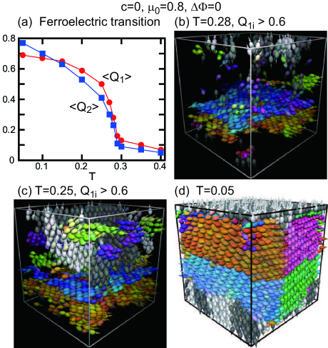
Figure 2: Ferroelectric transition in one-component dipole system (${c=0}$) with $\mu_{0}=0.8$ without applied field ($\Delta\Phi=0$). (a) Average orientational order parameters $\langle{Q_{1}}\rangle$ and $\langle{Q_{2}}\rangle$ in Eq.(24) vs $T$, where a ferroelectric transition is steep but gradual due to multi-domain states in a film system with fixed width $H=21.2$. (b) Ordered regions with $Q_{1i}>0.6$ at $T=0.28$ and (c) those at $T=0.25$ in a disordered matrix, where the fraction of the ordered regions expands with lowering $T$. (d) Rhombohedral polycrystalline state at $T=0.05$.

III Ferroelectric transition for $c=0$

We first examine a ferroelectric transition in crystal composed of dipolar spheroids with $\eta=1.2$ in Eq.(4) without impurities. See similar simulation by Johnson et al.Johnson1 for the prolate case with aspect ratio 1.25.

It is convenient to introduce orientational order parameters defined for each dipole $i$ as

$$Q_{\ell i}=\sum_{j\in{\rm neighbor}}P_{\ell}({\mbox{\boldmath$n$}}_{i}\cdot{\mbox{\boldmath$n$}}_{j})/Z_{i}\quad(\ell=1,2),$$ (24)

where $P_{1}(x)=x$ and $P_{2}(x)=(3x^{2}-1)/2$. We sum over neighbor dipoles $j$ with $r_{ij}<1.4$, where $Z_{i}$ is their number. Then, $Q_{1i}$ represents the local dipolar order and $Q_{2i}$ the local quadrupolar orderBinder ; ori . These variables will be used also for ferroelectric glass with $c>0$.

In Fig.2, we examine the transition by slowly lowering $T$ for ${c=0}$, $\mu_{0}=0.8$, and $\Delta\Phi=0$. In (a), we plot the averages $\langle{Q_{1}}\rangle=\sum_{i\in 1}Q_{1i}/N_{1}$ and $\langle{Q_{2}}\rangle=\sum_{i\in 1}Q_{2i}/N_{1}$. Here, the transition is steep but gradual due to the finite-size effect imposed by the metal walls at $z=0$ and $H$. In our system, the spheroidal particles form a fcc crystal in the plastic crystal phase Binder ; ori ; EPL in the range $0.3<T<1$. For lower $T$, a polycrystal with eight rhombohedral variants appears, where the spheroid directions ${\mbox{\boldmath$n$}}_{i}$ are along $\langle{111}\rangle$ except those near the interfaces.

In the transition range $0.22\lesssim T\lesssim 0.30$, the system is composed of disordered and ordered regions with sharp interfaces. We give snapshots of relatively ordered regions with $Q_{1i}>0.6$ at (b) $T=0.28$ and (c) $T=0.25$, where we pick up (b) 10$\%$ and (c) $30\%$ of the total dipoles. These patterns are stationary in our simulation time intervals. In (d), at $T=0.05$, we give a snapshot of polycrystal state with eight variants.

The rhombohedral structure is characterized by the angles $\pi/2\pm\alpha$ of its lozenge faces of a unit cell. At low $T$, we find $\alpha\cong 5^{\circ}$ for $\mu_{0}=0.8$ but $\alpha\cong 1^{\circ}$ for $\mu_{0}=1.6$. See Sec.VA for the reason of this $\mu_{0}$ dependence.

IV Ferroelectric transition for $c>0$

IV.1 Role of impurities

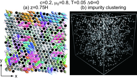
Figure 3: (a) Cross-sectional snapshot on $(111)$ ($xy$-plane) at $z=0.75H$ exhibiting planar anchoring of dipoles around impurities (black circles). (b) Distribution of impurities (white spheres) with diameter 0.22 (real diameter being 1.1). Bonds (white lines) are written between impurity pairs if $r_{ij}<1.4$. In these panels, $c=0.2$, $\mu_{0}=0.8$, $T=0.05$, and $\Delta\Phi=0$.

The impurities hinder the spheroid rotations and suppress long-range orientational order not affecting the crystal order. In our previous papers Takae-ori ; EPL , this gave rise to orientational glass without electrostatic interactions. In a mixture of nematogenic molecules and large spherical particles, surface anchoring of the former around the latter suppresses the long-range nematic order Jun .

In Fig.3(a), we display the dipole directions for c=0.2 on a (111) plane at $z=0.75H$. Many of them tend to align in the directions parallel to the impurity surfaces or perpendicular to ${\mbox{\boldmath$r$}}_{ij}$ ($j\in 2$), because $A_{ij}=0$ for ${\mbox{\boldmath$n$}}_{i}\cdot{\mbox{\boldmath$r$}}_{ij}=0$ in Eq.(3). However, this anchoring is possible only partially, because the dipoles are on the lattice points and the impurities form clusters. This picture resembles those of PNRs on crystal surfaces of relaxors Ann ; Bokov2 ; Bokov4 .

In Fig.3(b), we display all the impurities in the cell for $c=0.2$, where clustering is significant. As guides of eye, we write bonds between pairs of impurities if their distance is smaller than 1.4. In this bond criterion, we find large clusters composed of many members $(\gtrsim 10)$ including a big one percolating through the cell. These clusters were pinned during crystallization, so they depend on the potentials and the cooling rate. They strongly influence the shapes of PNRs (see Figs.9 and 10 also).

Correlated quenched disorder should also be relevant in real systems. For relaxors, much effortWel ; Wel1 ; Ban has been made to determine the distribution of the B-site ions (Mg²⁺ and Nb⁵⁺ for PMN) using effective atom-atom interactions, while Burton et al. Burton1 ; Burton2 ; Burton3 demonstrated strong influence of compositional heterogeneity on the PNRs.

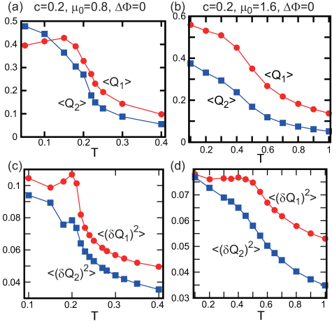
Figure 4: Diffuse ferroelectric transition with impurities for $c=0.2$ and $\Delta\Phi=0$. Top: $\langle{Q_{1}}\rangle$ and $\langle{Q_{2}}\rangle$ vs $T$ for (a) $\mu_{0}=0.8$ and (b) $\mu_{0}=1.6$. Bottom: $\langle{(\delta Q_{1})^{2}}\rangle$ and $\langle{(\delta Q_{2})^{2}}\rangle$ vs $T$ for (c) $\mu_{0}=0.8$ and (d) $\mu_{0}=1.6$.

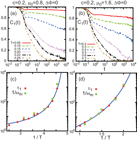
Figure 5: Slow orientational dynamics with impurities for $c=0.2$ and $\Delta\Phi=0$. Top: Time-correlation function $C_{1}(t)$ in Eq.(26) for (a) $\mu_{0}=0.8$ and (b) $\mu_{0}=1.6$ at several temperatures. Bottom: Orientational relaxation time $\tau_{1}(T)$ from Eq.(27) (red circles) and inverse frequency $1/\omega_{\rm m}(T)$ vs $1/T$ from Eq.(29) (green boxes) for (c) $\mu_{0}=0.8$ and (d) $\mu_{0}=1.6$, indicating $\tau_{1}\omega_{\rm m}\sim 1$. As a guide of eye, data of $\tau_{1}$ are fitted to Vogel-Fulcher form (28) (bold line).

IV.2 Diffuse transition toward ferroelectric glass

The dipole moment $\mu_{0}$ determines relative importance of the dipolar and steric parts, ${\mbox{\boldmath$E$}}_{i}$ and ${\mbox{\boldmath$E$}}_{i}^{\rm ste}$, in the orientating field in Eq.(21), since they are proportional to $\mu_{0}$ and $\mu_{0}^{-1}$, respectively, for $E_{\rm a}=0$. For example, for $c=0.2$ and $\Delta\Phi=0$, we average (${|{\mbox{\boldmath$E$}}_{i}|}$, ${|{\mbox{\boldmath$E$}}_{i}^{\rm ste}|}$) over all the dipoles to obtain ($2.0$, $5.7$) for $\mu_{0}=0.8$ and $T=0.1$ and ($4.6$, $3.4$) for $\mu_{0}=1.6$ and $T=0.2$. Thus, ${\mbox{\boldmath$E$}}_{i}$ is more important for larger $\mu_{0}$ in the dipole orientations. Here, the amplitude of the local electric field $|{\mbox{\boldmath$E$}}_{i}|$ is mostly of order $4\pi\mu_{0}n_{1}/3=2.8\mu_{0}$, where $n_{1}=(1-c)N/V$. This large size of ${\mbox{\boldmath$E$}}_{i}$ is realized within mesoscopic PNRs.

In Fig.4, we examine the transition with $c=0.2$ and $\Delta\Phi=0$ for the two cases $\mu_{0}=0.8$ and $1.6$, where the net polarization nearly vanishes. At each $T$, we waited for a time $\Delta t\sim 5\times 10^{4}$. In (a) and (b) we show gradual $T$ dependence of $\langle{Q_{\ell}}\rangle=\sum_{i\in 1}Q_{\ell i}(t_{0})/N_{1}$. They take appreciable values in the presence of small PNRs. In (c) and (d), we also show their variances,

$$\langle{(\delta Q_{\ell})^{2}}\rangle=\sum_{i\in 1}(Q_{\ell i}(t_{0})-\langle{Q_{\ell}}\rangle)^{2}/N_{1}\quad(\ell=1,2).$$ (25)

The orientation fluctuations are frozen at large sizes at low $T$. We also see that $\langle{Q_{1}}\rangle$ in (a) and $\langle{(\delta Q_{1})^{2}}\rangle$ in (c) exhibit small maxima at low $T$, but they should disappear in the ensemble averages.

In Fig.5, we plot the time-correlation functions $C_{1}(t)$ for one-body angle changes defined by

$$C_{1}(t)=\sum_{i\in 1}\langle{{\mbox{\boldmath$n$}}_{i}(t_{0})\cdot{\mbox{\boldmath$n$}}_{i}(t_{0}+t)}\rangle/N_{1},$$ (26)

where the average is taken over the initial time $t_{0}$. In (a) and (b), the angle changes slow down with lowering $T$. We define the reorientation time $\tau_{1}$ by

$$C_{1}(\tau_{1})=0.1,$$ (27)

where 0.1 is smaller than the usual choice $e^{-1}$ since $C_{1}(t)$ decays considerably in the initial thermal stage for not very low $T$. The PNRs are broken on this timescale. In (c) and (d), we display $\tau_{1}$ vs $1/T$. where $\tau_{1}$ can well be fitted to the Vogel-Fulcher form Kob ,

$$\tau_{1}=\tau_{10}\exp[D_{1}T_{1}/(T-T_{1})].$$ (28)

Here, $\tau_{10}$, $T_{1}$, and $D_{1}$ are constants with $(D_{1},T_{1})$ being $(0.89,0.19)$ for $\mu_{0}=0.8$ and $(4.7,0.32)$ for $\mu_{0}=1.6$.

IV.3 Dielectric permittivity

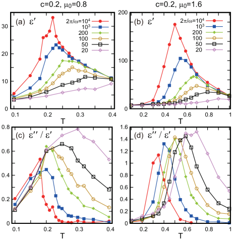
Figure 6: Frequency-dependent dielectric permittivity for $2\pi/\omega=10^{4},10^{3},200,10^{2}$, 50, and $20$ with $c=0.2$ and $\Delta\Phi=0$. Top: $\varepsilon^{\prime}(\omega,T)$ vs $T$ for (a) $\mu_{0}=0.8$ and (b) $\mu_{0}=1.6$, which exhibits a maximum $\varepsilon^{\prime}_{m}(\omega)$ at $T=T_{\rm m}(\omega)$. Bottom: $\varepsilon^{\prime\prime}(\omega,T)/\varepsilon^{\prime}(\omega,T)$ vs $T$ for (c) $\mu_{0}=0.8$ and (d) $\mu_{0}=1.6$.

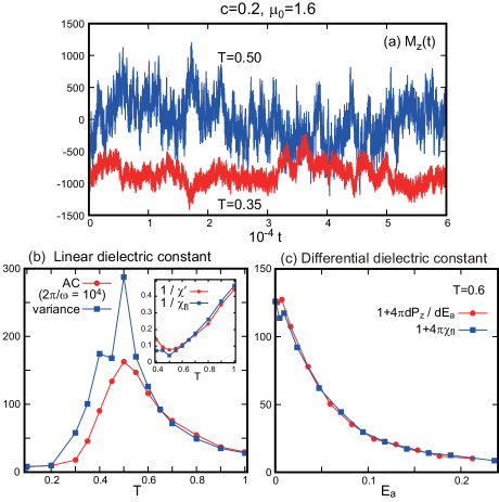
Figure 7: Ergodicity and nonergodicity for $c=0.2$ and $\mu_{0}=1.6$. (a) Time evolution of $M_{z}(t)$ at $T=0.5$ (blue) and 0.35 (red) with $\Delta\Phi=0$. (b) $\varepsilon^{\prime}(\omega,T)=1+4\pi\chi^{\prime}$ (red) and $\varepsilon_{\rm fl}=1+4\pi\chi_{\rm fl}$ (blue), where $\varepsilon^{\prime}$ is from ac response at $\omega=2\pi\times 10^{-4}$ in Fig.6(b) and $\chi_{\rm fl}$ is the normalized variance of $\delta M_{z}$ in Eq.(30) for $\Delta\Phi=0$. Two curves coincide for $T>T_{\rm m}(\omega)$, but disagree for lower $T$. Shown also are $1/\chi^{\prime}$ and $1/\chi_{\rm fl}$ (inset), indicating Eq.(31). (c) Coincidence of $\varepsilon_{\rm fl}=1+4\pi\chi_{\rm fl}$ and $\chi_{\rm dif}=1+4\pi dP_{z}/dE_{\rm a}$ as functions of $E_{\rm a}$ at $T=0.6$.

We next examine the dielectric permittivity. We calculated its real part $\varepsilon^{\prime}(\omega,T)$ and imaginary part $\varepsilon^{\prime\prime}(\omega,T)$ as functions of $T$ and the frequency $\omega$ by applying small ac field in the linear response regime (see Appendix B).

In Fig.6, we show $\varepsilon^{\prime}$ and the ratio $\varepsilon^{\prime\prime}/\varepsilon^{\prime}$ vs $T$ at several low frequencies for the two cases $\mu_{0}=0.8$ (left) and 1.6 (right). In (a) and (b), $\varepsilon^{\prime}$ increases with decreasing $\omega$ and exhibit a broad maximum at a temperature $T=T_{\rm m}(\omega)$ for each $\omega$. With decreasing $\omega$, $T_{\rm m}(\omega)$ decreases (with weaker dependence for smaller $\omega$) and the peak height $\varepsilon^{\prime}_{\rm m}(\omega)=\varepsilon^{\prime}(\omega,T_{\rm m}(\omega))$ increases. For $T>T_{\rm m}$, we have $\omega<\tau_{1}^{-1}$, so $\varepsilon^{\prime}(\omega,T)$ tends to the linear dielectric constant $\varepsilon(T)$. However, for $T<T_{\rm m}$, $\varepsilon^{\prime}$ decreases to zero with lowering $T$ or increasing $\omega$, where the response of the PNRs to small ac field decreases. On the other hand, $\varepsilon^{\prime\prime}/\varepsilon^{\prime}$ exhibits a maximum for each $\omega$ and shifts to a lower temperature with lowering $\omega$. These behaviors characterize ferroelectric glass Cr ; Cr1 ; Smo ; Klee ; Klee1 ; Zhang ; Cowley ; Bokov ; Bokov3 ; Samara ; Loidl3 ; Ho2 . Similar behaviors were found for the frequency-dependent magnetic susceptibilities in spin glassMydosh . Furthermore, in Appendix B, we will present analysis of $\varepsilon^{\prime}$ and $\varepsilon^{\prime\prime}$ for $\omega\gtrsim\tau_{1}^{-1}$ at relatively high $T$ on the basis of the linear response theoryKubo .

We write the inverse relation of $T=T_{\rm m}(\omega)$ as

$$\omega=T_{\rm m}^{-1}(T)=\omega_{\rm m}(T),$$ (29)

leading to $\varepsilon^{\prime}(\omega_{\rm m},T)=\varepsilon_{\rm m}^{\prime}(\omega_{\rm m})$. Here, $T/T_{\rm m}>1$ ($<1$) holds for $\omega/\omega_{\rm m}<1$ ($>1$). In (c) and (d) of Fig.5, we compare the inverse $1/\omega_{\rm m}(T)$ and $\tau_{1}(T)$ in Eq.(27) for $\mu_{0}=0.8$ and 1.6. We find $\omega_{\rm m}\sim\tau_{1}^{-1}$. Thus, $\omega_{\rm m}(T)$ represents a characteristic frequency of the dipole reorientations. Previously, for relaxors and spin glasses, Stringer et al.Ra nicely fitted $1/\omega_{\rm m}(T)$ to the Vogel-Fulcher form, which is in accord with (c) and (d) of Fig.5.

Our system is ergodic at relatively high $T$, but becomes nonergodic as $T$ is lowered. The boundary between these two regimes weakly depends on the observation time. In Fig.7(a), $M_{z}(t)$ evolves on a wide range of time scales in a time interval with width $6\times 10^{4}$ for $c=0.2$, $\Delta\Phi=0$, and $\mu_{0}=1.6$. At $T=0.5$, its time average becomes small, but its fluctuations are large. In contrast, at $T=0.35$, it remains negative around $-800=-14(Vk_{\rm B}T)^{1/2}$, on which smaller thermal fluctuations with faster time scales are superimposed. Note that the ensemble average of $M_{z}$ should vanish at any $T$ for $\Delta\Phi=0$.

For a single simulation run, we consider the time average of the normalized polarization variance, written as $\chi_{\rm fl}$. To avoid confusion, we define it explicitly as

$$Vk_{\rm B}T\chi_{\rm fl}={{\langle{(\delta M_{z})^{2}}\rangle}_{\rm time}}={\langle{M_{z}^{2}}\rangle}_{\rm time}-{\langle{M_{z}}\rangle}_{\rm time}^{2}.$$ (30)

We set ${\langle{{\cal A}}\rangle}_{\rm time}=\int_{t_{1}}^{t_{2}}dt{\cal A}(t)/\Delta t$ with $\Delta t=t_{2}-t_{1}(\sim 5\times 10^{4}$ here) for any time-dependent variable ${\cal A}(t)$. This averaging procedure has already been taken for the quantities in Figs.4 and 5. In the nonergodic $T$ range, ${\langle{M_{z}}\rangle}_{\rm time}$ remains nonvanishing even for $\Delta\Phi=0$, while $\chi_{\rm fl}$ arises from the (thermal) dynamical fluctuations and tends to zero as $T\to 0$. In Fig.7(b), we plot numerical results of $\varepsilon_{\rm fl}=1+4\pi\chi_{\rm fl}$ for $\Delta\Phi=0$ and $\varepsilon^{\prime}=1+4\pi\chi^{\prime}$ at $\omega=2\pi\times 10^{-4}$ as functions of $T$. These two curves nearly coincide for $T>T_{\rm m}$ yielding $\varepsilon(T)$, but $\varepsilon_{\rm fl}$ is considerably larger than $\varepsilon^{\prime}$ for $T<T_{\rm m}$. In their simulation, Burton et al.Burton1 ; Burton2 calculated a dielectric constant from polarization fluctuations, which corresponds to $\varepsilon_{\rm fl}$ in our case.

In Fig.7(b), $\varepsilon_{\rm fl}$ and $\varepsilon^{\prime}$ steeply grow as $T\to T_{\rm m}$. From the curves of $1/\chi^{\prime}$ and $1/\chi_{\rm fl}$ in its inset, $\chi^{\prime}=(\varepsilon^{\prime}-1)/4\pi$ and $\chi_{\rm fl}$ can fairly be fitted to the Curie-Weiss form,

$$\chi^{\prime}\cong\chi_{\rm fl}\cong A_{0}/(T-T_{0}),$$ (31)

with $A_{0}\cong 1.2$ and $T_{0}\cong 0.47(\cong T_{\rm m}$ at $\omega=2\pi\times 10^{-4}$) for $T\gtrsim 0.55$. At $T=0.5$, however, we find $\chi^{\prime}\cong 13$ and $\chi_{\rm fl}\cong 23$. In experiments, the behavior (31) was found for orientational glassori , but a marked deviation was detected close to $T_{\rm m}$ for relaxorsSamara ; Bokov ; Cr1 . Thus, if $T$ is somewhat above $T_{0}$, our polarization fluctuations resemble the critical fluctuations in systems near their critical point Cowley ; Samara . In our disordered system, these near-critical fluctuations are slowed down and eventually frozen as $T$ is further lowered, as in relaxors. This can also be seen in (c) and (d) of Fig.4. Furthermore, for $T\lesssim T_{0}$, there is a tendency of interface formation between adjacent PNRs for $c\lesssim 0.2$, which will be discussed in future.

For relaxors, Stock et al.Stock divided the scattering intensity into frozen and dynamic parts, where the former (latter) increases (decreases) with lowering $T$. Similar arguments of nonergodicity were made for polymer gelsPusey ; Matsuo , where the fluctuations of the polymer density consist of frozen and dynamic parts. Moreover, if gelation takes place in a polymer solution close to its criticality, the critical concentration fluctuations are pinned at the network formation Matsuo ; Onukibook .

We next confirm Eq.(17) by increasing $E_{\rm a}$ at $T=0.6$ with $c=0.2$ and $\mu_{0}=1.6$, where the observation time is much longer than $\tau_{1}\sim 60$. In Fig.7(c), we compare the differential formula $\varepsilon_{\rm dif}=1+4\pi dP_{z}/dE_{\rm a}$ and the fluctuation formula $\varepsilon_{\rm fl}=1+4\pi\chi_{\rm fl}$ for the field-dependent dielectric constant. The former is calculated from the data in Fig.12(a) and the latter from Eq.(30), where these two curves are surely very close. At this $T$, the polarization fluctuations are suppressed with increasing $E_{\rm a}$.

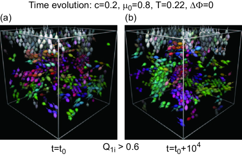
Figure 8: Time evolution of PNRs in the ergodic regime, where $T=0.22$, $c=0.2$, and $\mu_{0}=0.8$ (see (a) and (c) of Fig.5). Displayed are snapshots of dipoles with $Q_{1i}>0.6$ at (a) $t=t_{0}$ and (b) $t=t_{0}+10^{4}$ in the same simulation run, which amount to $14\%$ of the total dipoles. These patterns are different, so they have lifetimes shorter than $10^{4}$.

IV.4 Polar nanoregions in diffuse transition

In our diffuse transition, the PNRs are relatively ordered regions consisting of aligned clusters enclosed by impurities. At relatively high $T$, they have finite lifetimes (within observation times)Bokov ; Bl . This feature is illustrated in two snapshots in Fig.8, which were taken at two times separated by $10^{4}$ in the same simulation run. They display the dipoles with $Q_{1i}>0.6$ for $T=0.22$, $c=0.2$, and $\mu_{0}=0.8$. These two patterns are very different, so their lifetime is shorter than $10^{4}$. In fact, $\tau_{1}$ is of order $10^{3}$ at $T=0.22$ in Fig.5(c).

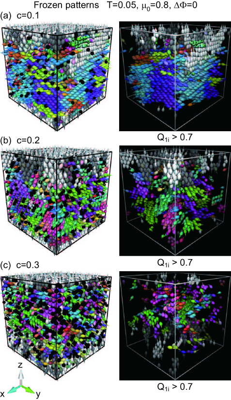
Figure 9: Frozen PNRs at $T=0.05$ for (a) $c=0.1$ (top), (b) $c=0.2$ (middle), and (c) $c=0.3$ (bottom) with $\mu_{0}=0.8$ and $\Delta\Phi=0$. Left: Dipoles (in color) and impurities (in black) on the boundaries ($x,y,{\rm or}~{}z=L)$. Right: Dipoles with $Q_{1i}>0.7$ forming PNRs, whose typical sizes decrease with increasing $c$.

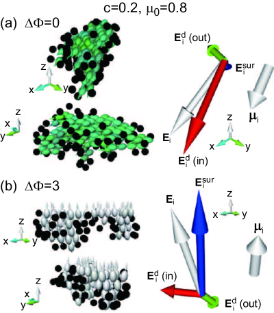
Figure 10: Left: Frozen PNRs surrounded by impurities (black spheres) viewed from two directions for (a) $\Delta\Phi=0$ at the cell center and for (b) $\Delta\Phi=3$ near the top wall, where $c=0.2$, $\mu_{0}=0.8$, and $T=0.05$. Right: Local electric field ${\mbox{\boldmath$E$}}_{i}$ in Eq.(13) and dipole moment ${\mbox{\boldmath$\mu$}}_{i}$ of a typical dipole $i$ within the left PNRs. Here, ${\mbox{\boldmath$E$}}_{i}$ consists of the field from the surface charges ${\mbox{\boldmath$E$}}_{i}^{\rm sur}$ and those from the dipoles inside and outside the PNR, ${\mbox{\boldmath$E$}}_{i}^{\rm d}$(in) and ${\mbox{\boldmath$E$}}_{i}^{\rm d}$(out). In (a), ${\mbox{\boldmath$E$}}_{i}\cong{\mbox{\boldmath$E$}}_{i}^{\rm d}({\rm in})$ and ${\mbox{\boldmath$E$}}_{i}^{\rm sur}$ is small. In (b), ${\mbox{\boldmath$E$}}_{i}\cong{\mbox{\boldmath$E$}}_{i}^{\rm sur}$.

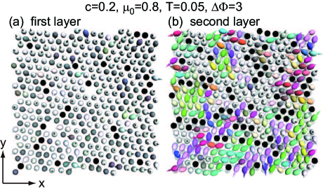
Figure 11: Orientations of dipoles on $(111)$ planes near the bottom metal wall for $c=0.2$, $\mu_{0}=0.8$, and $T=0.05$ with $\Delta\Phi=3$ ($E_{\rm a}=0.14$). Displayed are cross-sectional snapshots in (a) the first layer ($0<z_{i}<1$) and (b) the second layer ($1<z_{i}<2$), where black circles represent impurities. In (a), the fraction of the dipoles parallel (antiparallel) to the $z$ axis is $65\%$ ($35\%$). In (b), the oblique orientations appear.

The PNRs are frozen with lowering $T$. In Fig.9, we give examples for $c=0.1$, 0.2, and 0.3 with $T=0.05$, $\mu_{0}=0.8$, and $\Delta\Phi=0$. The left panels display the particles on the boundaries ($x,y,{\rm or}~{}z=L$), while the right ones the relatively ordered dipoles with $Q_{1i}>0.7$. The dipoles depicted in the latter amount to 37, 20, and 13$\%$ of the total dipoles from above. For $c=0.1$, we can see well-defined ordered domains consisting of eight variants, whose interfaces are trapped at impuritiesEPL ; Takae-ori (see Fig.10(a)). These domains are broken up into smaller PNRs with increasing $c$. For $c=0.2$, the PNRs mostly take compressed, plate-like shapes under the constraint of the spatially correlated impurities (see Fig.10 also). For $c=0.3$, the dipole orientations are highly frustrated on the particle scale without well-defined interfaces.

To be quantitative, we define PNRs as follows. In each PNR, any member $i$ satisfies $Q_{1i}>0.7$ and $r_{ij}<1.4$ for some $j$ within the same PNR. In Fig.9, the dipole number in a PNR is $2200,270$, and $56$ on the average from above. Thus, the connectivity of the PNRs sensitively depends on $c$. In the following, we treat the case $c=0.2$.

IV.5 Single polar nanoregion and local electric field

We visualize individual PNRs frozen at low $T$. When the system is composed of PNRs, the local electric field ${\mbox{\boldmath$E$}}_{i}$ in Eq.(13) arises mainly from the dipoles within the same PNR in the bulk. Its amplitude is of order $4\pi\mu_{0}n_{1}/3\cong 2.8\mu_{0}$ for not very large $\Delta\Phi$.

In Fig.10, we pick up (a) a single PNR for $\Delta\Phi=0$ at the cell center and (b) another one for $\Delta\Phi=3$ ($E_{\rm a}=0.14$) near the upper wall, where $c=0.2$ and $T=0.05$. We depict the impurities whose distance to some dipole in the PNR is shorter than 1.4. We find the numbers of the constituent dipoles and impurities as (a) $(120,70)$ and (b) $(70,50)$ using the definition of PNRs in Sec.IVD. Here, the dipoles tend to be parallel to the impurity surfaces, as discussed in Sec.IVA, and almost all the impurities are on the PNR boundaries, resulting in plate-like PNRs.

In Fig.10 (right), we choose a typical dipole in the PNR interior (not in contact with the impurities) and display its ${\mbox{\boldmath$E$}}_{i}$ and ${\mbox{\boldmath$\mu$}}_{i}$, where they are nearly parallel. Here, we divide the dipolar part of ${\mbox{\boldmath$E$}}_{i}$ into the contributions from those inside and outside the PNR, written as ${\mbox{\boldmath$E$}}_{i}^{\rm d}(\rm{in})$ and ${\mbox{\boldmath$E$}}_{i}^{\rm d}(\rm{out})$. Then, Eq.(A9) in Appendix A gives

$${\mbox{\boldmath$E$}}_{i}={\mbox{\boldmath$E$}}_{i}^{\rm d}({\rm in})+{\mbox{\boldmath$E$}}_{i}^{\rm d}({\rm out})+{\mbox{\boldmath$E$}}_{i}^{\rm sur},$$ (32)

where the last term arises from the surface charges. In (a), we find ${\mbox{\boldmath$E$}}_{i}\cong{\mbox{\boldmath$E$}}_{i}^{\rm d}(\rm{in})$, which occurs mostly for the dipoles in the interior of PNRs in the bulk. In (b), on the other hand, we find ${\mbox{\boldmath$E$}}_{i}\cong{\mbox{\boldmath$E$}}_{i}^{\rm sur}$, where $|{\mbox{\boldmath$E$}}_{i}^{\rm sur}|$ is of the same order as $4\pi{\bar{\sigma}}_{0}=2.4$ and is much larger than $E_{\rm a}=0.14$. Here, ${\bar{\sigma}}_{0}$ is the mean surface charge density at $z=0$. For example, if we set $\epsilon/k_{\rm B}=100$ K and $\sigma_{1}=5~{}{\rm\AA}$, we have ${\bar{\sigma}}_{0}\sim 0.01e/\sigma_{1}^{2}$. for $\Delta\Phi=3$.

IV.6 Orientation near metal surface

As can be seen in Figs.9 and 10(b), the dipoles next to the walls are parallel or antiparallel to the $z$ axis (along $[111]$), whose distances from the walls are about 0.5. This is due to their interaction with the image dipoles in the walls (see Appendix A)Takae1 ; Takae2 ; apply . For $\Delta\Phi=0$, these two orientations appear equally on the average due to the top-tail symmetry of our spheroidal dipoles. For $\Delta\Phi\neq 0$, one of them is more preferred than the other. In Fig.11, we show the particles in the first and second $(111)$ layers in applied field with $\Delta\Phi=3$, where $c=0.2$, $\mu_{0}=0.8$, and $T=0.05$. The parallel and antiparallel orientations appear in the first layer, but the other oblique ones also appear in the second layer. We shall see that the corresponding surface charge density $\sigma_{0}(x,y)$ at $z=0$ is highly heterogeneous in Fig.17 in Appendix A.

In our crystal case, the $\ell$-th layer is given by $\ell-1<z<\ell$, since the separation between adjacent $(111)$ planes is close to 1. Here, we consider the average of $n_{zi}=\cos\theta_{i}$ over the dipoles in the $\ell$-th layer and write it as $\langle{n_{z}}\rangle_{\ell}$. In Fig.11, it is 0.30 for $\ell=1$, $0.34$ for $\ell=2$, and $\langle{n_{z}}\rangle_{\rm b}=0.33$ for $\ell\gg 1$. These values are close, so the surface effect on the polarization is weak in this case of our model. The excess potential drop near the bottom wall is given by $4\pi\mu_{0}n_{1}\sigma_{1}\sum_{\ell}[\langle{n_{z}}\rangle_{\rm b}-\langle{n_{z}}\rangle_{\ell}]\cong 0.13$, which is much smaller than the total drop $\Delta\Phi=3$. In contrast, for highly polar liquids such as water Hautman ; Takae2 ; Willard , a significant potential drop appears in a microscopic (Stern) layer on a solid surface even without ion adsorption.

V Polarization and strain in applied electric field

V.1 Applying electric field along $[111]$ at fixed stress

In this section, we give results of cyclic changes of $\Delta\Phi=HE_{\rm a}$ for $c=0.2$ and $\mu_{0}=1.6$. We also calculated the response with $\mu_{0}=0.8$ (not shown here). For these two $\mu_{0}$ values, the characteristic features are nearly the same, but the response sizes are very different. That is, the dielectric response for $\mu_{0}=1.6$ is larger than that for $\mu_{0}=0.8$ by one order of magnitude as in Fig.6, while the field-induced strain for $\mu_{0}=1.6$ is about $20\%$ of that for $\mu_{0}=0.8$. See the last paragraph of Sec.III for the rhombohedral angles in our simulation. Using a barostat, we fixed the $zz$ component of the average stress and varied the cell width $H(t)$ to calculate the field-induced strain. The lateral cell length was fixed at $L$.

In our model, dipole alignment along $[111]$ yields both steric repulsion and dipolar attraction between adjacent $(111)$ planes. Their relative importance depends on $\mu_{0}$. If the former is larger (smaller) than the latter, an expansion (a shrinkage) of the cell width $H$ occurs for $\Delta\Phi\neq 0$. Note that the dipolar interaction between two dipoles at ${\mbox{\boldmath$r$}}_{i}$ and ${\mbox{\boldmath$r$}}_{j}$ aligned along the $z$ axis is attractive (repulsive) if the angle between their relative vector ${\mbox{\boldmath$r$}}_{i}-{\mbox{\boldmath$r$}}_{j}$ and the $z$ axis is smaller (larger) than $\cos^{-1}(1/\sqrt{3})$.

We increased $\Delta\Phi(t)$ from 0 to 10, decreased to $-10$, and then increased again to 10 at fixed $T$ without dislocation formation. The changing rate ${\dot{\Phi}}=d(\Delta\Phi)/dt$ was $\pm 1.5\times 10^{-3}$ $\epsilon/(\sigma_{1}^{3}m)^{1/2}$. The average pressure along the $z$ axis was 0.4 at $T=0.2$ and 3.6 at $T=0.6$ in units of $\epsilon/\sigma_{1}^{3}$, while the lateral one increased by 0.8 for a change of $\Delta\Phi$ from 0 to 10. The $H(t)$ changed from $H(0)=L$ at most by $2\%$. We calculated the average polarization and strain for $t>0$ given by

$${P}_{z}(t)={M_{z}}(t)/[L^{2}H(t)],\quad\bar{\gamma}(t)=H(t)/L-1.$$ (33)

We also calculated the mean surface charge density ${\bar{\sigma}}_{0}$ at $z=0$ to confirm Eq.(A5) in Appendix A (see Fig.12).

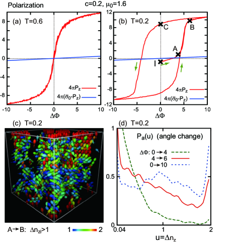
Figure 12: Polarization $P_{z}$ to cyclic applied electric field $E_{\rm a}(t)\cong\Delta\Phi(t)/21$ for $c=0.2$ and $\mu_{0}=1.6$. Top: $4\pi{{P}}_{z}$ vs $\Delta\Phi(t)$ at (a) $T=0.6$ and (b) $T=0.2$. Straight lines in (a) and (b) (in blue) represent $4\pi({\bar{\sigma}}_{0}-{P}_{z})$, which coincide with $E_{\rm a}$. Bottom: (c) Snapshot of the dipoles with large angle changes $\Delta n_{zi}>1$ between two points A and B ($\Delta\Phi:4\to 6$) in (b), where $n_{zi}$ is the $z$ component of ${\mbox{\boldmath$n$}}_{i}$. Colors represent $\Delta n_{zi}$ according to the color bar. (d) Distribution $P_{\rm a}(u)$ for $u=\Delta n_{zi}=n_{zi}(t_{1})-n_{zi}(t_{0})$ between two points in the cycle in (b). Small angle changes are dominant in the initial interval ($\Delta\Phi:0\to 4$) (green line), but large angle changes are dominant in the subsequent one ($\Delta\Phi:4\to 6$) (red line).

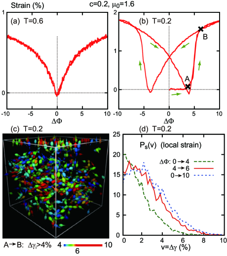
Figure 13: Average strain $\bar{\gamma}$ to applied electric field for $c=0.2$ and $\mu_{0}=1.6$. Top: ${\bar{\gamma}}$ vs $\Delta\Phi(t)$ at (a) $T=0.6$ and (b) $T=0.2$. (c) Snapshot of the dipoles whose changes in the local strain $\Delta\gamma_{i}$ in Eq.(35) exceed $0.04$ between two points A and B in (b). Colors represent $\Delta\gamma_{i}$ according to the color bar. (d) Distribution $P_{\rm s}(v)$ for strain changes $v=\Delta\gamma_{i}=\gamma_{i}(t_{1})-\gamma_{i}(t_{0})$ between two times in (b). It is narrower for the initial interval ($\Delta\Phi:0\to 4$) (green line) than for the subsequent one ($\Delta\Phi:4\to 6$) (red line).

V.2 Polarization response

In Fig.12, we plot $4\pi{P}_{z}$ vs $\Delta\Phi$ for (a) $T=0.6$ and (b) $T=0.2$. At $\Delta\Phi=10$, we have $P_{z}\sim 10$ and $\langle{n_{z}}\rangle=P_{z}/n_{1}\mu_{0}\sim 0.75$ in (a) and (b), where $n_{zi}$ is the $z$ component of ${\mbox{\boldmath$n$}}_{i}$ and $n_{1}=N_{1}/V$ is $0.672$. In (a), there is no hysteresis and the initial slope yields $\varepsilon_{\rm dif}=1+4\pi dP_{z}/dE_{\rm a}\cong 153$. In (b), marked hysteresis appears, where $\varepsilon_{\rm dif}\cong 13$ initially at point I, but is about $150$ between two points A and B ($\Delta\Phi:4\to 6$). Here, the initial $P_{z}$ at I is slightly negative as a frozen fluctuation (see the curve at $T=0.35$ in Fig.7(a)). At point C on the vertical axis we have a remnant polarization $P_{\rm R}=0.72$ with $\Delta\Phi=0$. For any $T$, $\varepsilon_{\rm dif}$ from the initial slope at $E_{\rm a}=0$ nearly coincides with $\varepsilon^{\prime}$ at $\omega=2\pi\times 10^{-4}$ in Fig.7(b) (equal to 50 at $T=0.4$ and to 10 at $T=0.1$). The curves in (a) and (b) closely resemble those in various ferroelectric systems Bl ; Mori ; Furukawa ; Zhang ; piezo .

The field-induced change from A to B in (b) is very steep with large $\chi_{\rm dif}$. In (c), we thus display the dipoles with large angle changes: $\Delta n_{zi}=n_{zi}(t_{B})-n_{zi}(t_{A})>1$, where $t$ is $t_{A}$ at A and $t_{B}$ at B. Collective reorientations are marked in this time interval. In (d), for three intervals, we plot the distribution function $P_{\rm a}(u)=\sum_{i\in 1}{\delta(u-\Delta n_{zi})}/N_{1}$ for $\Delta n_{zi}=n_{zi}(t_{1})-n_{zi}(t_{0})$, where we use an appropriately smoothed $\delta$-function. Small angle changes are dominant in the first interval $t_{I}<t<t_{A}$ (where $t=t_{I}$ at I), but large angle changes are dominant in the next interval $t_{A}<t<t_{B}$.

In (b), the initial point I (at $t=t_{I}$) of the cycle represents an arrested state with frozen fluctuations realized by zero-field cooling. It can no longer be reached once a large field is applied. The corresponding states have been realized in many systems (see Sec.VI). In the two states at I and C, the polarization directions are very different, but the values of the potential energy $U$ in Eq.(2) are close as $-8.07N\epsilon$ at I and $-8.04N\epsilon$ at C. We can also see that the quadrupolar order parameters $Q_{2i}(t)$ in Eq.(24) do not change much for most $i$ during the cycle despite large changes in ${\mbox{\boldmath$n$}}_{i}$. For example, the mean square difference $\sum_{i}[Q_{2i}(t_{I})-Q_{2i}(t)]^{2}/N_{1}$ for time interval $[t_{I},t]$ is $0.047$, $0.103$, and $0.086$ at $t=t_{A}$, $t_{B}$, and $t_{C}$ (which are the times at A, B, and C), respectively, where the variance $\sum_{i\in 1}[\delta Q_{2i}(t)]^{2}/N_{1}$ for $\delta Q_{2i}=Q_{2i}-\langle{Q_{2}}\rangle$ remains of order 0.08 (see Eq.(25) and Fig.4d)

Between A and B in (b), we found an increase in the polarization variance $\langle{(\delta M_{z})^{2}}\rangle(t)$ $(t_{A}\lesssim t\lesssim t_{B}$). For relaxors, Xu et al. Shi2 detected an increase in the diffuse scattering in the field range with large $\chi_{\rm dif}$. We should then examine the scattering amplitude between A and B. In addition, when $\Delta\Phi$ was held fixed at 4.0 (at A), we observed slow reorientations leading to coarsening of PNRsaging ; aging0 . These effects will be studied in future.

V.3 Field-induced strain

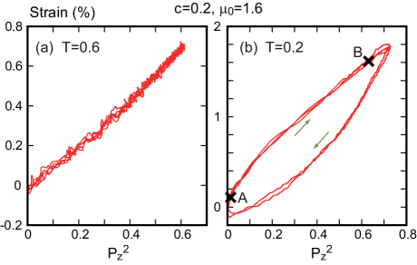
Figure 14: Average strain ${\bar{\gamma}}$ vs ${P}_{z}^{2}$ for $c=0.2$ and $\mu_{0}=1.6$. (a) At $T=0.6$, electrostriction relation ${\bar{\gamma}}\propto P_{z}^{2}$ holds. (b) At $T=0.2$, a closed loop appears, where points A and B corresponds to A and B in (b) of Figs.12 and 13.

In our model, the heterogeneity in the strain is marked because of dilation of PNRs along $\langle{111}\rangle$, though it is milder than that of the polarization. To illustrate this effect, we define a local strain $\gamma_{i}$ along the $z$ axis for each particle $i$ (including the impurities) by

$$\gamma_{i}=\sum_{j}|z_{j}-z_{i}|/({W}_{i}a_{111})-1,$$ (34)

where the summation is over other $j$ with $r_{ij}<1.4$ and $|z_{j}-z_{i}|>0.2$, ${W}_{i}$ is the number of these neighbors, and $a_{111}(\cong 1.0)$ is the average spacing between two consecutive $(111)$ planes. From these conditions, the $(111)$ plane containing $j$ is adjacent to that containing $i$. The particle average $\sum_{i}\gamma_{i}/N$ nearly coincides with $\bar{\gamma}$ in Eq.(33).

In Fig.13, we plot $\bar{\gamma}$ vs $\Delta\Phi$ with $\mu_{0}=1.6$ in the same simulation run as in Fig.12. We find (a) a cusp curve at $T=0.6$ and (b) a butterfly-like curve at $T=0.2$. In (b), $\bar{\gamma}$ becomes slightly negative at $\Delta\Phi\cong\pm 4$. These two curves resemble those in the previous experiments Furu1 ; Zhang ; piezo . In (c), we pick up the particles with large local strain changes $\Delta\gamma_{i}=\gamma_{i}(B)-\gamma_{i}(A)>0.04$ between two points A and B at $T=0.2$ in (b), where $\bar{\gamma}$ is $0.016$ at B. We define the distribution function, $P_{\rm s}(v)=\sum_{i}{\delta(v-\Delta\gamma_{i})}/N$ for strain changes $\Delta\gamma_{i}=\gamma_{i}(t_{1})-\gamma_{i}(t_{0})$ between two times in (b). In (d), it is narrower for the initial interval ($\Delta\Phi:0\to 4$) than for the subsequent one ($\Delta\Phi:4\to 6$).

The shapes of our dipolar spheroids are centrosymmetric, leading to the electrostriction relation,

$$\bar{\gamma}\cong C_{\rm es}P_{z}^{2},$$ (35)

at relatively high $T$. In Fig.14, Eq.(35) nicely holds with $C_{\rm es}\cong 0.012\sigma_{1}^{3}/\epsilon$ at $T=0.6$, while a closed loop appears at $T=0.2$. If we set $\epsilon/k_{\rm B}=100$ K and $\sigma_{1}=5~{}{\rm\AA}$, our $C_{\rm es}$ becomes 10 m${}^{4}/$C². For ferroelectric polymers, Eq.(35) was found with a negative coefficient Zhang ; Z1 ; Furu1 ; Bl ($-13.5$ m${}^{4}/$C² after electron irradiationZhang ). In contrast, the piezoelectric relation ($\bar{\gamma}\propto P_{z}$) holds for relaxors above the transitionpiezo .

VI ZFC$/$FC temperature changes

A large number of ZFC$/$FC experiments have been performed, where $T$ is varied at zero or fixed ordering field (electric fieldWest ; Uesu ; Z1 ; Ho1 , magnetic fieldF0 ; F1 ; F4 , and stressF5 ; F3 ). However, the physical pictures of these processes remain unclear. Here, we show relevance of collective, large-angle orientational changes in these cycles.

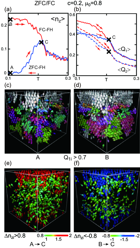
Figure 15: Results of ZFC-FH and FC-FH thermal cycles for $c=0.2$ and $\mu_{0}=0.8$, where $\Delta\Phi=0.5$ on the paths of FC and FH and $T=0.1$ at points A and B. (a) $\langle{n_{z}}\rangle=\langle{\cos\theta}\rangle$ vs $T$. (b) $\langle{Q_{1}}\rangle$ and $\langle{Q_{2}}\rangle$ vs $T$. Dipoles with $Q_{1i}>0.7$ are depicted at A in (c) and at B in (d). Also depicted are dipoles with large angle changes, where $n_{zi}>0.8$ from A to C in (e) and $n_{zi}<-0.8$ from B to C in (f). Colors of these dipoles are given according to the bars below these panels.

We followed cycles in Fig.15(a) setting $dT/dt=\pm 10^{-5}$ at fixed volume with $c=0.2$ and $\mu_{0}=0.8$. In ZFC-FH, (i) we cooled the system from a high-$T$ state to a low-$T$ state (point A) with $\Delta\Phi={P}_{z}=0$ and then (ii) heated it with $\Delta\Phi=0.5$ ($E_{\rm a}=0.024$) back to the initial $T$. Subsequently, in FC-FH, (iii) we cooled the system to point B with $\Delta\Phi=0.5$ and then (iv) heated it back with $\Delta\Phi=0.5$ fixed. We set $T=0.1$ at A and B.

In (a), we plot $\langle{n_{z}}\rangle={P}_{z}/\mu_{0}n_{1}$ vs $T$ on the two paths. The two heating curves meet at a freezing point C, where $T$ is given by $T_{\rm f}=0.21$ and the relaxation time $\tau_{1}$ in Eq.(27) is of order $10^{4}$. This $T_{\rm f}$ is very close to $T_{\rm m}$ at $\omega=2\pi\times 10^{-4}$ in Fig.6(a). Far below $T_{\rm f}$, the two curves are largely separated indicating marked nonergodicity, while they coincide for $T>T_{\rm f}$ in the ergodic regime.

In (b), we display $\langle{Q_{\ell}}\rangle=\sum_{i\in 1}Q_{\ell i}/N_{1}$ ($\ell=1,2$) in the same simulation run. From Eq.(24) they represent the average dipolar and quadrupolar orders. The difference of $\langle{Q_{1}}\rangle$ in the two cycles is at most $30\%$, while that of $\langle{Q_{2}}\rangle$ is only about $5\%$. Note that $Q_{2i}$ are rather insensitive to collective reorientations for most $i$ (see Sec.VB).

In (c) and (d), the dipoles with $Q_{1i}>0.7$ are depicted at A and B. These two patterns look similar, but some PNRs in the same locations in A and B have different polarization directions (for example, $[1\bar{1}\bar{1}]$ in A and $[\bar{1}11]$ in B). In the present example, the potential energy $U$ is $-5.86N\epsilon$ at A and $-5.88N\epsilon$ at B. Their difference ($=-0.02N\epsilon$) is small, but is still 5 times larger than $-E_{\rm a}M_{z}(=-0.004N\epsilon)$ at B (see $U_{\rm d}$ in Eq.(11)). Note that large potential barriers exist for reorientations of PNRs from the configurations at A to those at B. These barriers decrease with increasing $E_{\rm a}$, but its present size 0.024 is small. If a much larger $E_{\rm a}$ is applied at A, there can be a transition to a ferroelectric stateBl ; Bobnar .

In (e) and (f), we display the dipoles with large angle changes from A to C and from B to C. They satisfy $\Delta n_{zi}(A\to C)=n_{zi}(C)-n_{zi}(A)>0.8$ in (e) and $\Delta n_{zi}(B\to C)=n_{zi}(C)-n_{zi}(B)<-0.8$ in (f), where $n_{zi}$ are the $z$ component of ${\mbox{\boldmath$n$}}_{i}$. These large-angle changes are collective and heterogeneous. This should be a universal feature in glass coupled with a phase transition.

On the two FH paths, the potential barriers between the two states at the same $T$ remain very large for $T<T_{\rm f}$. They can be overcome by thermal activations at $T=T_{\rm f}$ (at C), where the reorientation rate of PNRs should be comparable to the inverse of the observation time $\tau_{\rm obs}$. Estimating the former as the inverse of $\tau_{1}$ in Eq.(27) and setting $\tau_{\rm obs}\sim T/(dT/dt)$, we obtain

$$\tau_{1}\sim T/(dT/dt)\quad({\rm at~{}point}~{}C).$$ (36)

Indeed, we have $\tau_{1}=2.4\times 10^{4}\cong 1.1T/(dT/dt)$ at C. Here, $\tau_{1}$ at the freezing should decrease significantly for large $E_{\rm a}$ (not shown here). It follows that $T_{\rm f}$ at C decreases with increasing $\tau_{\rm obs}$. Note that this dependence is weak for long $\tau_{\rm obs}$ due to the abrupt $T$ dependence of $\tau_{1}$ at low $T$. It is well known that nucleation in a metastable state starts at an onset temperatureOnukibook , which is rather well defined for long $\tau_{\rm obs}$.

In Fig.15, we have used small $E_{\rm a}(=0.024$). However, cooling at a high electric field, Bobnar et al. Bobnar detected a field-induced ferroelectric transition. Such a phase transition can be predicted from a Ginzburg-Landau theory for $P_{z}$ including the field term $-E_{\rm a}P_{z}$ Bl ; Onukibook .

VII Antiferroelectric glass

So far we have treated ferroelectric glass. However, antiferroelectric order has been observed in mixtures containing cyanide units CN^- such as KBr-KCN at low $T$ Mertz ; ori ; Binder ; anti-Loidl . It is also known that antiparallel alignment freezes at low $T$ in polar globular molecules such as cyanoadamantane anti ; anti0 containing CN or betaine phosphateAlbers containing H₃PO₄ due to their mutual steric hindrance. These systems should become antiferroelectric glass at low $T$ even without impurities. Here, we consider a mixture of dipoles and impurities introducing a short-range interaction favoring antiparallel ordering.

Supposing top-tail asymmetry of the dipoles, we replace the factor $A_{ij}$ ($i\in\alpha$ and $j\in\beta$) in Eq.(3) by

$${A}^{\prime}_{ij}=A_{ij}+\delta_{\alpha 1}\delta_{\beta 1}J{\mbox{\boldmath$n$}}_{i}\cdot{\mbox{\boldmath$n$}}_{j}.$$ (37)

The second term yields an exchange interaction between dipoles $i$ and $j$, where positive (negative) $J$ favors antiferroelectric (ferroelectric) ordering. We performed simulation for $J=0.1$ with $c=0.2$, $\mu_{0}=0.8$, and $\Delta\Phi=0$.

In Fig.16(a), we plot $\langle{Q_{1}}\rangle$ and $\langle{Q_{2}}\rangle$. Here, due to antiferroelectric ordering, $\langle{Q_{1}}\rangle$ remains very small at any $T$, but $\langle{Q_{2}}\rangle$ increases up to 0.42 with lowering $T$. Thus, the system exhibits quadrupolar order without dipolar order at zero applied electric field Binder ; ori . In more detail, we show the distribution functions $P_{\ell}(Q_{\ell})=\langle{\sum_{i\in 1}\delta(Q_{\ell}-Q_{\ell i})/N_{1}}\rangle$ at $T=0.05$. In (b), $P_{1}(Q_{1})$ is nearly symmetric (even) with respect to $Q_{1}\to-Q_{1}$ and $P_{2}(Q_{2})$ has a maximum at $Q_{2}\cong 1$ leading to $\langle{Q_{2}}\rangle\sim 0.4$.

Furthermore, in (c), a snapshot of the dipoles and the impurities is given, which looks very complicated. In (d), we show a typical antiferroelectric nanoregion in the middle of the cell, which are viewed from two directions. Any dipole $i$ in this region satisfies $\mbox{\boldmath$n$}_{i}\cdot\mbox{\boldmath$n$}_{j}<-0.98$ for some nearby $j$ with $r_{ij}<1.4$ within the same region. It is composed of 170 dipoles and surrounded by 130 impurities with no impurities in its interior. In (d) and (e), cross-sectional particle configurations are displayed at $z=H/2+2$ and $H/2+3$, respectively. We can see antiferroelectric ordering unambiguously for the dipoles parallel or antiparallel to the $z$ axis (perpendicular to $(111)$), while the orientations apparently look irregular for those perpendicular to $(\bar{1}11)$, $(1\bar{1}1)$, or $(11\bar{1})$.

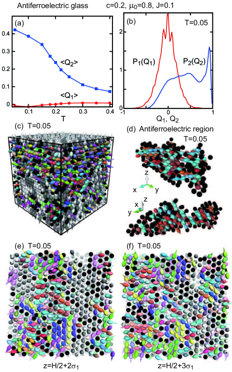
Figure 16: Antiferroelectric glass for $c=0.2$, $\mu_{0}=0.8$, $\Delta\Phi=0$, and $J=0.1$, where $\langle{Q_{1}}\rangle$ is small but $\langle{Q_{2}}\rangle$ increases gradually with lowering $T$ in (a). (b) Distributions $P_{\ell}(Q_{\ell})$ in Eq.(38) at $T=0.05$, which give $\langle{Q_{1}}\rangle\cong 0$ and $\langle{Q_{2}}\rangle\cong 0.42$. (c) Snapshot of dipoles and impurities (black spheres) at $T=0.05$. (d) Antiferroelectric nanoregion viewed from two directions. In (e) and (f), displayed are cross-sectional particle configurations at $z=H/2+2$ and $H/2+3$, respectively, at $T=0.05$.

VIII Summary and remarks

With molecular dynamics simulation, we have studied dipolar glass in mixtures of dipolar spheroids and apolar impurities in applied electric field. Properly calculating the electrostatics, we have visualized polar nanoregions (PNRs) and clarified their role in the dielectric response. We summarize our main results as follows.

(i) In Sec.II, we have introduced orientation-dependent Lennard-Jones potentials mimicking spheroidal repulsion. For its mild aspect ratio, the particles first form a fcc plastic crystal. Then, at lower $T$, the spheroids align along $\langle{111}\rangle$ resulting in rhombohedral structures. Assuming that each spheroid has a dipole parallel to its long axis, we have constructed an electrostatic energy $U_{\rm d}$ in Eq.(11), which accounts for the image dipoles and the applied field $E_{\rm a}$. In equilibrium, the differential susceptibility $\chi_{\rm dif}=dP_{z}/dE_{\rm a}$ is related to the polarization fluctuations as in Eq.(17).

(ii) In Sec.III, we have presented results on a structural phase transition in a one-component system of dipolar spheroids. It changes from a fcc crystal to a polycrystal with eight rhombohedral variants. This transition occurs in a narrow temperature range due to the finite size effect imposed by the metal walls.

(iii) In Sec.IV, we have examined diffuse ferroelectric transitions. The impurity distribution has been determined during crystallization, so marked impurity clustering has appeared. In our model, ferroelectric domains are broken up into smaller PNRs with increasing the impurity concentration $c$. For $c=0.2$, we have calculated the orientational time correlation function $C_{1}(t)$ in Fig.5 and the dielectric permittivity in Fig.6. The temperature of maximum of $\varepsilon^{\prime}$ is written as $T_{\rm m}(\omega)$. For very small $\omega$, the polarization fluctuations are enhanced for $T>T_{\rm m}$, but are composed of frozen PNRs and thermal fluctuations for $T<T_{\rm m}$. Individual PNRs have been visualized in Fig.10. The surface effects on the dipole orientations and the local electric fields have been examined in Sec.IVF and Appendix A.

(iv) In Sec.V, we have examined the polarization and the strain to cyclic applied electric field. At relatively high $T$, there is no hysteresis and an electrostriction relation holds. At low $T$, the polarization is on a hysteresis loop. In the cycle, collective large-angle changes are dominant where $\chi_{\rm dif}=dP_{z}/dE_{\rm a}$ is large.

(v) In Sec.VI, we have investigated the ZFC-FH and FC-FH thermal cycles in accord with the previous experiments. The frozen states at the lowest $T$ in the two cycles have been visualized in Fig.15. On the FH paths, heterogeneous collective reorientations have been found. These paths meet at a temperature $T_{\rm f}$, at which the reorientation rate ($\sim\tau_{1}^{-1})$ is of the same order as the ramping rate of the temperature ($\sim(dT/dt)/T$).

(vi) In Sec.VII, we have investigated antiferroelectric glass by introducing a short-ranged exchange interaction stemming from molecular shape asymmetry. We have visualized a typical antiferroelectric nanoregion.
(vii) In Appendix B, we have shown the method of calculating $\varepsilon^{\prime}$ and $\varepsilon^{\prime\prime}$ and found their algebraic behavior $(\propto\omega^{-\beta})$ at relatively large $\omega$ in the ergodic $T$ range.

Finally, we remark on future problems. (1) The isochoric specific heat $C_{V}$ can be calculated from the average energy. We found that it has a rounded peak in our mixture systems (not shown in this paper). This is consistent with the behavior of the isobaric specific heat $C_{p}$ in previous experiments ori ; Mertz ; Kawaji ; Tachibana . (2) There is a gradual crossover in the polarization fluctuations in the diffuse transition. For example, the PNRs have no clear boundaries at relatively high $T$, while sharp interfaces can appear at low $T$. It is of interest how the space correlations in the polarization and the particle displacements depend on $T$. (3) In real systems, impurities or mixed components have charges or dipoles. In solids, the polarization response can be large when ion displacements occur within unit cells as a phase transition. These features should be accounted for in future simulations. (4) Intriguing critical dynamics exists in the ergodic $T$ rangeKlee1 ; Bokov3 ; Bokov4 ; Cowley , as suggested by Eq.(31). The aging and memory effects at low $T$aging0 ; aging should also be studied in future (see the last paragraph of Sec.VB).

Acknowledgments
This work was supported by KAKENHI 15K05256, and KAKENHI 25000002. The numerical calculations were preformed on CRAY XC40 at YITP in Kyoto University and on SGI ICE XA/UV at ISSP in the University of Tokyo.

Appendix A: Electrostatics of dipole systems

Here, we explain the electrostatics of dipoles between metal walls in applied field Takae1 ; Takae2 ; Hautman ; apply ; Klapp . The electric potential due to the image dipoles is equivalent to that due to the surface charge densities, written as $\sigma_{0}(x,y)$ at $z=0$ and $\sigma_{H}(x,y)$ at $z=H$. Without adsorption and ionization on the surfaces, the dipole centers are somewhat away from the walls (see the comment below Eq.(6)). Then,

$$4\pi\sigma_{0}={E_{z}(x,y,0)},\quad 4\pi\sigma_{H}=-{E_{z}(x,y,H)},$$ (A1)

where $E_{z}=-\partial\Phi/\partial z$. We consider the 2D Fourier expansions of $\sigma_{\lambda}$. For $\lambda=0$ and $H$ they are

$$\sigma_{\lambda}({\mbox{\boldmath$r$}}_{\perp})={\bar{\sigma}}_{\lambda}+\sum_{{\mbox{\boldmath$k$}}\neq{\mbox{\boldmath$0$}}}\sigma_{\lambda{\mbox{\boldmath$k$}}}\exp[{{\rm i}{\mbox{\boldmath$k$}}\cdot{\mbox{\boldmath$r$}}_{\perp}}],$$ (A2)

where ${\mbox{\boldmath$r$}}_{\perp}=(x,y)$, and ${\mbox{\boldmath$k$}}=(2\pi/L)(n_{x},n_{y})\neq(0,0)$ with $n_{x}$ and $n_{y}$ being integers. The first term is the mean surface charge density ${\bar{\sigma}}_{\lambda}=\int_{0}^{L}dx\int_{0}^{L}dy~{}\sigma_{\lambda}(x,y)/L^{2}$. From Eq.(10) we can express the Fourier components $\sigma_{\lambda{\mbox{\boldmath$k$}}}$ asapply

$$\sigma_{\lambda{\mbox{\boldmath$k$}}}=-\sum_{j}({\mbox{\boldmath$\mu$}}_{j}\cdot\nabla_{j})[G_{k}^{\lambda}(z_{j})e^{-{\rm i}{\mbox{\boldmath$k$}}\cdot{\mbox{\boldmath$r$}}_{j}}]/L^{2},$$ (A3)

where $\nabla_{j}=\partial/\partial{\mbox{\boldmath$r$}}_{j}$, $G_{k}^{0}(z)={\sinh(k(H-z))}/\sinh(kH)$, and $G_{k}^{H}(z)={\sinh(kz)}/\sinh(kH)$ with $k=|{\mbox{\boldmath$k$}}|$.

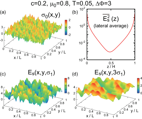
Figure 17: Surface charge effects in ferroelectric glass for $\mu_{0}=0.8$, $c=0.2$, $T=0.05$, and $\Delta\Phi=3$. (a) $\sigma_{0}(x,y)$ on the $xy$ plane at $z=0$ exhibiting both microscopic and mesoscopic fluctuations, (b) Lateral average $\overline{E_{\rm s}^{2}}$ in Eq.(A12) vs $z/H$. (c) $E_{\rm s}$ on the $xy$ plane at $z=1$, and (d) that at $z=3$. Here, $E_{\rm s}=|\nabla\phi_{\rm s}|$ arises from the surface charge deviations decaying far from the walls, but the nanodomain contribution to $E_{\rm s}$ exceeds the microscopic part with increasing $z$.

For dipolar systems, the Poisson equation is written as

$$\nabla^{2}\Phi=4\pi\nabla\cdot\sum_{i}{\mbox{\boldmath$\mu$}}_{i}\delta({\mbox{\boldmath$r$}}-{\mbox{\boldmath$r$}}_{i}).$$ (A4)

Integration of Eq.(A4) in the cell yields ${\bar{\sigma}}_{0}+{\bar{\sigma}}_{H}=0$. We also multiply Eq.(A4) by $z$ and integrate it in the cell. Using the total polarization $M_{z}$ we findHautman ; Takae1

$$\bar{\sigma}_{0}=-\bar{\sigma}_{H}=E_{\rm a}/4\pi+M_{z}/V,$$ (A5)

without surface adsorption and ionization. The fluctuations of ${\bar{\sigma}}_{0}$ and $M_{z}/V$ thus coincide at fixed $E_{\rm a}$ Hautman ; apply ; Takae1 ; Takae2 .

The mean surface charge densities produce the potential $-4\pi{\bar{\sigma}}_{0}z$ in the cell, so $\Phi$ consists of three parts as

$$\Phi({\mbox{\boldmath$r$}})=\Phi_{\rm d}({\mbox{\boldmath$r$}})-4\pi{\bar{\sigma}}_{0}z+\phi_{\rm s}({\mbox{\boldmath$r$}}),$$ (A6)

which is equivalent to Eq.(10). The first term $\Phi_{\rm d}$ arises from the dipoles in the cell. Imposing the lateral periodic boundary condition, we express it as

$$\Phi_{\rm d}({\mbox{\boldmath$r$}})=\sum_{{\mbox{\boldmath$m$}}_{\perp}}{\sum_{i}}{\mbox{\boldmath$g$}}({{\mbox{\boldmath$r$}}-{\mbox{\boldmath$r$}}_{i}+L{\mbox{\boldmath$m$}}_{\perp}})\cdot{\mbox{\boldmath$\mu$}}_{i},$$ (A7)

where ${\mbox{\boldmath$g$}}({\mbox{\boldmath$r$}})=r^{-3}{\mbox{\boldmath$r$}}$ and ${\mbox{\boldmath$m$}}_{\perp}=(m_{x},m_{y},0)$ with $m_{x}$ and $m_{y}$ being integers. The third term $\phi_{\rm s}$ in Eq.(A6) arises from the charge density deviations $\delta\sigma_{\lambda}(x,y)=\sigma_{\lambda}-{\bar{\sigma}}_{\lambda}$. In terms of $\sigma_{\lambda{\mbox{\boldmath$k$}}}$ in Eq.(A2), $\phi_{\rm s}$ is expressed as

$$\phi_{\rm s}=\frac{2\pi}{L^{2}}\sum_{{\mbox{\boldmath$k$}}\neq{\mbox{\boldmath$0$}}}\frac{1}{k}e^{{\rm i}{\mbox{\boldmath$k$}}\cdot{\mbox{\boldmath$r$}}_{\perp}}\bigg{[}\sigma_{0{\mbox{\boldmath$k$}}}e^{-kz}+\sigma_{H{\mbox{\boldmath$k$}}}e^{-k(H-z)}\bigg{]}.$$ (A8)

Now the local electric field ${\mbox{\boldmath$E$}}_{i}$ is written as

$${\mbox{\boldmath$E$}}_{i}={\mbox{\boldmath$E$}}_{i}^{\rm d}+{\mbox{\boldmath$E$}}_{i}^{\rm sur}.$$ (A9)

The first term arises from the other dipoles in the cell:

$${\mbox{\boldmath$E$}}_{i}^{\rm d}=-\sum_{{\mbox{\boldmath$m$}}_{\perp}}{\sum_{j}}^{\prime}{\stackrel{{\scriptstyle\leftrightarrow}}{{\mbox{\boldmath$\cal T$}}}}({{\mbox{\boldmath$r$}}_{ij}+L{\mbox{\boldmath$m$}}_{\perp}})\cdot{{\mbox{\boldmath$\mu$}}_{j}},$$ (A10)

The second term is due to the surface charges:

$${\mbox{\boldmath$E$}}_{i}^{\rm sur}=-4\pi{\bar{\sigma}}_{0}{\mbox{\boldmath$e$}}_{z}+{\mbox{\boldmath$E$}}_{\rm s}({\mbox{\boldmath$r$}}_{i}),$$ (A11)

where the first term is homogeneous and ${\mbox{\boldmath$E$}}_{\rm s}({\mbox{\boldmath$r$}})=-\nabla\phi_{\rm s}({\mbox{\boldmath$r$}})$ is due to $\delta{\sigma_{\lambda}}={\sigma_{\lambda}}-{{\bar{\sigma}}_{\lambda}}$. The dipoles next to the walls are parallel or antiparallel to the $z$ axis due to ${\mbox{\boldmath$E$}}_{\rm s}$ even for $\Delta\Phi=0$ (see the snapshots in this paper)apply . However, as in Fig.17(b), ${\mbox{\boldmath$E$}}_{\rm s}$ is negligibly small (even in ferroelectric states) if the distances from the walls exceed the typical domain size. This is due to the factors $\exp({-kz})$ and $\exp(-k(H-z))$ in Eq.(A8).

In Fig.17, we show (a)$\sigma_{0}(x,y)$, (b)$\overline{E_{\rm s}^{2}}(z)$, (c)$E_{\rm s}(x,y,1)$, and (d)$E_{\rm s}(x,y,3)$ in ferroelectric glass of our system, where we set $E_{\rm s}(x,y,z)=|{\mbox{\boldmath$E$}}_{\rm s}|=|\nabla\phi_{\rm s}|$ and

$$\overline{E_{\rm s}^{2}}=\int_{0<x,y<L}dxdyE_{\rm s}(x,y,z)^{2}/L^{2}.$$ (A12)

Here, $\sigma_{0}(x,y)$ in (a) and $E_{\rm s}(x,y,1)$ in (c) consist of microscopic and mesoscopic fluctuations. The latter arise from the PNRs near the surface from Fig.11, being apparent in (d). For $z$ longer than the PNR length, $E_{\rm s}(x,y,z)$ decays to zero in (b). Thus, ${\mbox{\boldmath$E$}}_{i}^{\rm sur}\to-4\pi{\bar{\sigma}}_{0}{\mbox{\boldmath$e$}}_{z}$ far from the walls, which was previously found for liquid waterTakae1 ; Takae2 .

Appendix B: Linear response to oscillating field and frequency-dependent susceptibilities

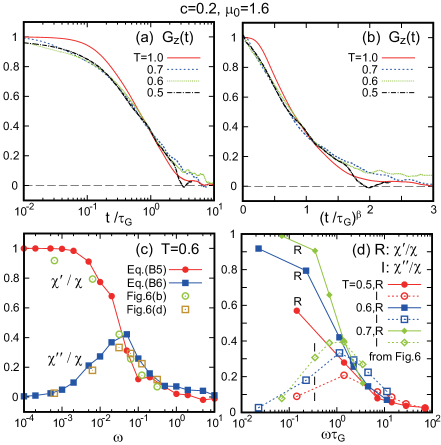
Figure 18: Dielectric relaxation for $c=0.2$ and $\mu_{0}=1.6$. (a) $G_{z}(t)$ in Eq.(B4) vs $t/\tau_{G}$ at $T=0.5,0.6,0.7$, and 1.0 on a semi-logarithmic scale, where $\tau_{G}$ is determined by $G_{z}(\tau_{G})=e^{-1}$. (b) $G_{z}(t)$ vs $(t/\tau_{G})^{\beta}$ with $\beta=0.57$ on a linear scale. (c) $\chi^{\prime}(\omega)/\chi$ and $\chi^{\prime\prime}(\omega)/\chi$ vs $\omega$ from one-sided Fourier transformation of $G_{z}(t)$ (filled symbols) and those from data in Fig.6 (open symbols). (d) $\chi^{\prime}(\omega)/\chi$ (R) and $\chi^{\prime\prime}(\omega)/\chi$ (I) vs $\omega\tau_{G}$ at $T=0.5$, 0.6, and 0.7 from data in Fig.6.

We applied a small sinusoidal electric field of the form $E_{\rm a}(t)=E_{\rm a}^{1}\sin(\omega t)$ with $E_{\rm a}^{1}=0.047$. We calculated the polarization response $\delta P_{z}=\delta M_{z}/V$ to this perturbation over 10 periods. After a few periods, it is expressed as

$$\delta{P_{z}}(t)=[\chi^{\prime}(\omega)\sin(\omega t)-\chi^{\prime\prime}(\omega)\cos(\omega t)]E_{\rm a}^{1},$$ (B1)

where $\chi^{\prime}$ and $\chi^{\prime\prime}$ are the frequency-dependent susceptibilities. Then, $\varepsilon^{\prime}$ and $\varepsilon^{\prime\prime}$ in Fig.6 are defined by

$$\varepsilon^{\prime}=1+4\pi\chi^{\prime},\quad\varepsilon^{\prime\prime}=4\pi\chi^{\prime\prime}.$$ (B2)

The Hamiltonian ${\cal H}$ increases as ${\overline{d{\cal H}/dt}}=V\omega\chi^{\prime\prime}|E_{\rm a}^{1}|^{2}/2$ in time (see below Eq.(20)), where the time average is taken in one period. From Eq.(A5) the mean surface charge density at the bottom wall is written as

$$\delta\langle{{\bar{\sigma}_{0}}}\rangle(t)=[\varepsilon^{\prime}\sin(\omega t)-\varepsilon^{\prime\prime}\cos(\omega t)]E_{\rm a}^{1}/4\pi,$$ (B3)

which oscillates as $\sin(\omega t-\delta_{\rm p})$ with $\tan\delta_{\rm p}=\varepsilon^{\prime\prime}/\varepsilon^{\prime}$. In Fig.6, we give the resultant $\varepsilon^{\prime}$ and $\varepsilon^{\prime\prime}/\varepsilon^{\prime}$ in a wide $T$ range including the nonergodic range.

On the other hand, around equilibrium, we can use the linear response theory Kubo for the Hamiltonian of the form (15). Within this scheme, the dielectric response can be expressed in terms of the time-correlation function for the deviation $\delta M_{z}(t)=M_{z}(t)-{\langle{M_{z}}\rangle}_{\rm e}$:

$$G_{z}(t)={\langle{\delta M_{z}(t+t_{0})\delta M_{z}(t_{0})}\rangle}_{\rm e}/Vk_{\rm B}T\chi,$$ (B4)

where ${\langle{\cdots}\rangle}_{\rm e}$ represents the equilibrium average and $\chi={\langle{(\delta M_{z})^{2}}\rangle}_{\rm e}/Vk_{\rm B}T=(\varepsilon-1)/4\pi$ at $E_{\rm a}=0$ (see Eq.(17)). Using $G_{z}(t)$ we obtain the linear response relations,

$$\chi^{\prime}(\omega)/\chi = 1-\omega\int_{0}^{\infty}dtG_{z}(t)\sin(\omega t),$$ (B5)

$$\chi^{\prime\prime}(\omega)/\chi = \omega\int_{0}^{\infty}dtG_{z}(t)\cos(\omega t).$$ (B6)

The complex susceptibility $\chi^{\prime}-i\chi^{\prime\prime}$ can be expressed as

$$\chi^{\prime}(\omega)-i\chi^{\prime\prime}(\omega)=-\chi\int_{0}^{\infty}dt{\dot{G}}_{z}(t)e^{-i\omega t},$$ (B7)

in terms of the time derivative ${\dot{G}}_{z}(t)={dG_{z}(t)}/{dt}$.

In Fig.18(a), we show our numerical results of $G_{z}(t)$ in Eq.(B4) at $T=0.5,0.6,0.7$, and 1.0 for $c=0.2$, $\Delta\Phi=0$, and $\mu_{0}=1.6$, where the data at long times are inaccurate, however. From $G_{z}(\tau_{G})=e^{-1}$, we define the relaxation time $\tau_{G}$, which is somewhat shorter than $\tau_{1}$ in Fig.5. In fact, we obtain $(\tau_{G},\tau_{1})=(230,1300),(36,60)$, $(11,17)$, and $(1.8,2.5)$ for $T=0.5,0.6$, 0.7, and 1.0, respectively. We may introduce another time by $\tau^{\prime}_{G}=\lim_{\omega\to 0}\chi^{\prime\prime}/\omega\chi=\int_{0}^{\infty}dtG_{z}(t)$, but we confirm $\tau_{G}^{\prime}\sim\tau_{G}$.

In (b), the initial decay of $G_{z}(t)$ is well fitted to

$$G_{z}(t)=1-A_{\rm p}(t/\tau_{G})^{\beta}+\cdots\quad(t\lesssim\tau_{G}),$$ (B8)

where $\beta\cong 0.57$ and $A_{\rm p}\cong 0.63$. Then, ${\dot{G}}_{z}(t)\propto-t^{\beta-1}$ for $t\lesssim\tau_{G}$. If this is substituted into Eq.(B7), we find

$${\chi^{\prime}(\omega)}-i\chi^{\prime\prime}(\omega)\cong B_{\rm p}e^{-i\pi\beta/2}(\omega\tau_{G})^{-\beta}\quad(\omega\tau_{G}\gtrsim 1),$$ (B9)

where $B_{\rm p}=\beta\Gamma(\beta)A_{\rm p}\chi\sim\chi$. The algebraic form (B9) with $0<\beta<1$ has been observed in many systems including relaxors and mixed crystals Bokov3 ; Klee ; ori .

We calculated the ratios $\chi^{\prime}(\omega)/\chi$ and $\chi^{\prime\prime}(\omega)/\chi$ from Eqs.(B5) and (B6) using $G_{z}(t)$ in (a). In (c), they are plotted at $T=0.6$ together with those from the data in Fig.6, where the latter are from Eq.(B1). The points from these two sets fairly agree for any $\omega$. In (d), we also plot these ratios vs $\omega\tau_{G}$ at three temperatures using the results in Fig.6. The behaviors in the region $\omega\tau_{G}\gtrsim 1$ in (c) and (d) support the algebraic form (B9).

References

- (1) Wei D and Patey G N 1992 Phys. Rev. A 46 7783
- (2) Weis J J and Levesque D 1993 Phys. Rev. E 48 3728
- (3) Tao R 1993 Phys. Rev. E 47 423
- (4) Ayton G, Gingras M J P and Patey G N 1997 Phys. Rev. E 56 562
- (5) Gao G T and Zeng X C 2000 Phys. Rev. E 61 R2188
- (6) Teixeira P I C, Tavares J M and Telo da Gama M M 2000 J. Phys.: Condens. Matter 12 R411
- (7) Groh B and Dietrich S 2001 Phys. Rev. E 63 021203
- (8) Hynninen A-P and Dijkstra M 2005 Phys. Rev. Lett. 94 138303
- (9) Bartke J and Hentschke R 2006 Mol. Phys. 104 3057
- (10) Bartke J and Hentschke R 2007 Phys. Rev. E 75 061503
- (11) Johnson L E, Barnes R, Draxler T W, Eichinger B E and Robinson B H 2010 J. Phys. Chem. B 114 8431
- (12) Johnson L E, Benight S J, Barnes R and Robinson B H 2015 J. Phys. Chem. B 119 5240
- (13) Blinc R 2011 Advanced Ferroelectricity (New York: Oxford University Press)
- (14) Binder K and Kob W 2005 Glassy Materials and Disordered Solids (Singapore: World Scientific)
- (15) Vugmeister B E and Glinchuk M D 1990 Rev. Mod. Phys. 62 993
- (16) Smolensky G A 1970 J. Phys. Soc. Jpn. Suppl. 28 26
- (17) Cross L E 1987 Ferroelectrics 76 241
- (18) Samara G A 2003 J. Phys.: Condens. Matter 15 R367
- (19) Kleemann W 2006 J. Mater. Sci. 41 129
- (20) Kleemann W 2014 Phys. Stat. Sol. (b) 251 1993
- (21) Bokov A A and Ye Z-G 2006 J. Mater. Sci. 41 31
- (22) Bokov A A and Ye Z-G 2012 J. Adv. Dielectrics 2 1241010
- (23) Cowley R A, Gvasaliya S N, Lushnikov S G, Roessli B and Rotaru G M 2011 Adv. Phys. 60 229
- (24) Setter N and Cross L E 1980 J. Appl. Phys. 51 4356
- (25) Westphal V, Kleemann W and Glinchuk M D 1992 Phys. Rev. Lett. 68 847
- (26) Burns G and Dacol F H 1983 Phys. Rev. B 28 2527
- (27) Viehland D, Jang S J, Cross L E and Wuttig M 1992 Phys. Rev. B 46 8003
- (28) Stringer C J, Lanagan M J, Shrout T R and Randall C A 2007 Jpn. J. Appl. Phys. 46 1090
- (29) Xu G, Zhong Z, Hiraka H and Shirane G 2004 Phys. Rev. B 70 174109
- (30) Jeong I-K, Darling T W, Lee J K, Proffen Th, Heffner R H, Park J S, Hong K S, Dmowski W and Egami T 2005 Phys. Rev. Lett. 94 147602
- (31) Xu G, Zhong Z, Bing Y, Ye Z-G and Shirane G 2006 Nat. Mater. 5 134
- (32) Stock C, Van Eijck L, Fouquet P, Maccarini M, Gehring P M, Xu G, Luo H, Zhao X, Li J-F and Viehland D 2010 Phys. Rev. B 81 144127
- (33) Welberry T R, Goossens D J and Gutmann M J 2006 Phys. Rev. B 74 224108
- (34) Paściak M, Welberry T R, Kulda J, Kempa M and Hlinka J 2012 Phys. Rev. B 85 224109
- (35) Bursill L A, Qian H, Peng J and Fan X D 1995 Physica B 216 1
- (36) Fujishiro K, Iwase T, Uesu Y, Yamada Y, Dkhil B, Kiat J-M, Mori S and Yamamoto N 2000 J. Phys. Soc. Jpn. 69 2331
- (37) Fu D, Taniguchi H, Itoh M, Koshihara S, Yamamoto N and Mori S 2009 Phys. Rev. Lett. 103 207601
- (38) Shvartsman V V, Kleemann W, Łukasiewicz T and Dec J 2008 Phys. Rev. B 77 054105
- (39) Kalinin S V, Rodriguez B J, Jesse S, Morozovska A N, Bokov A A and Ye Z-G 2009 Appl. Phys. Lett. 95 092904
- (40) Bokov A A et al. 2011 Z. Kristallogr 226 99
- (41) Chen J, Chan H M and Harmer M P 1989 J. Am. Ceram. Soc. 72 593
- (42) Hilton A D, Barber D J, Randall C A and Shrout T R 1990 J. Mater. Sci. 25 3461
- (43) Perrin C, Menguy N, Bidault O, Zahra C Y, Zahra A-M, Caranoni C, Hilczer B and Stepanov A 2001 J. Phys.: Condens. Matter 13 10231
- (44) Jin H Z, Zhu J, Miao S, Zhang X W and Cheng Z Y 2001 J. Appl. Phys. 89 5048
- (45) Hchli U T, Knorr K and Loidl A 1990 Adv. Phys. 39 405
- (46) Binder K and Reger J D 1992 Adv. Phys. 41 547
- (47) Toulouse J, Vugmeister B E and Pattnaik R 1994 Phys. Rev. Lett. 73 3467
- (48) Hchli U T, Kofel P and Maglione M 1985 Phys. Rev. B 32 4546
- (49) Maglione M, Hchli U T and Joffrin J 1986 Phys. Rev. Lett. 57 436
- (50) Volkmann U G, Bhmer R, Loidl A, Knorr K, Hchli U T and Hausshl S 1986 Phys. Rev. Lett. 56 1716
- (51) Loidl A, Schrder T, Bhmer R, Knorr K, Kjems J K and Born R 1986 Phys. Rev. B 34 1238
- (52) Mertz B and Loidl A 1987 Europhys. Lett. 4 583
- (53) Hessinger J and Knorr K 1993 Phys. Rev. B 47 14813
- (54) Yokota H and Uesu Y 2007 J. Phys.: Condens. Matter 19 102201
- (55) Loidl A, Knorr K, Rowe J M and McIntyre G J 1988 Phys. Rev. B 37 389
- (56) Qian J, Hentschke R and Heuer A 1999 J. Chem. Phys. 110 4514
- (57) Takae K and Onuki A 2012 Europhys. Lett. 100 16006
- (58) Takae K and Onuki A 2014 Phys. Rev. E 89 022308
- (59) Lovinger A J 1983 Science 220 1115
- (60) Furukawa T, Date M and Fukada E 1980 J. Appl. Phys. 51 1135
- (61) Furukawa T and Seo N 1990 Jpn. J. Appl. Phys. 29 675
- (62) Zhang Q M, Bharti V and Zhao X 1998 Science 280 2101
- (63) Cheng Z-Y, Bharti V, Xu T-B, Xu H, Mai T and Zhang Q M 2001 Sens. Actuators A 90 138
- (64) Ji Y, Ding X, Lookman T, Otsuka K and Ren X 2013 Phys. Rev. B 87 104110
- (65) Burton B P, Cockayne E and Waghmare U V 2005 Phys. Rev. B 72 064113
- (66) Burton B P, Cockayne E, Tinte S, and Waghmare U V 2006 Phase Transitions 79 91
- (67) Tinte S, Burton B P, Cockayne E and Waghmare U V 2006 Phys. Rev. Lett. 97 137601
- (68) Klapp S H L 2006 Mol. Simul. 32 609
- (69) Takae K and Onuki A 2013 J. Chem. Phys. 139 124108
- (70) Hautman J, Halley J W and Rhee Y-J 1989 J. Chem. Phys. 91 467
- (71) Takae K and Onuki A 2015 J. Phys. Chem. B 119 9377
- (72) Takae K and Onuki A 2015 J. Chem. Phys. 143 154503
- (73) Mulder C A M, van Duyneveldt A J and Mydosh J A 1981 Phys. Rev. B 23 1384
- (74) Nagata S, Keesom P H and Harrison H R 1979 Phys. Rev. B 19 1633
- (75) Gayathri N, Raychaudhuri A K, Tiwary S K, Gundakaram R, Arulraj A and Rao C N R 1997 Phys. Rev. B 56 1345
- (76) Viehland D, Li J F, Jang S J, Cross L E and Wuttig M 1992 Phys. Rev. B 46 8013
- (77) Letz M, Schilling R and Latz A 2000 Phys.Rev. E 62 5173
- (78) Gay J G and Berne B J 1981 J. Chem. Phys. 74 3316
- (79) Kubo R 1957 J. Phys. Soc. Jpn. 12 570
- (80) Onuki A 2002 Phase Transition Dynamics (Cambridge: Cambridge University Press)
- (81) Alberici-Kious F, Bouchaud J P, Cugliandolo L, Doussineau P and Levelut A 1998 Phys. Rev. Lett. 81 4987
- (82) Kircher O and R. Bhmer 2002 Eur. Phys. J. B 26 329
- (83) Yamamoto J and Tanaka H 2001 Nature 409 321
- (84) Pusey P N and van Megen W 1989 Physica A 157 705
- (85) Matsuo E S, Orkistz M, Sun S-T, Li Y and Tanaka T 1994 Macromolecules 27 6791
- (86) Willard A P, Reed S K, Madden P A and Chandler D 2009 Faraday Discuss. 141 423
- (87) Park S-E and Shrout T R 1997 J. Appl. Phys. 82 1804
- (88) Bobnar V, Kutnjak Z, Pirc R and Levstik A 1999 Phys. Rev. B 60 6420
- (89) Amoureux J P, Castelain M, Benadda M D, Bee M and Sauvajol J L 1983 J. Physique 44 513
- (90) Foulon M, Amoureux J P, Sauvajol J L, Cavrot J P and Muller M 1984 J. Phys. C: Solid State Phys. 17 4213
- (91) Albers J, Klpperpieper A, Rother H J and Ehses K H 1982 Phys. Stat. Sol. (a) 74 553
- (92) Moriya Y, Kawaji H, Tojo T and Atake T 2003 Phys. Rev. Lett. 90 205901
- (93) Tachibana M and Takayama-Muromachi E 2009 Phys. Rev. B 79 100104(R)