Chiral pair fluctuations for the inhomogeneous chiral transition

Abstract

The effects of fluctuations are discussed around the phase boundary of the inhomogeneous chiral transition between the inhomogeneous chiral phase and the chiral-restored phase. The particular roles of thermal and quantum fluctuations are elucidated and a continuity of their effects across the phase boundary is suggested. In addition, it is argued that anomalies in the thermodynamic quantities should have phenomenological implications for the inhomogeneous chiral transition. Some common features for other phase transitions, such as those from the normal to the inhomogeneous Fulde-Ferrell-Larkin-Ovchinnikov state in superconductivity, are also emphasized.

I Introduction

The inhomogeneous chiral transition is one of the fascinating topics in the study of the QCD phase diagram fuk . Many people have believed that there may be the chiral transition in the chemical potential ($\mu$) and temperature ($T$) plane, while there has not yet been any direct evidence in addition to the fact that the lattice QCD simulations do not work at finite $\mu$ due to the so-called sign problem. The chiral transition essentially separates two phases: one is the spontaneous symmetry breaking (SSB) phase and the other is the symmetric (chiral-restored) phase. Besides these two phases, recent studies have suggested the appearance of the inhomogeneous chiral phase (iCP) as another possibility for the realization of chiral symmetry chi ; dcdw ; nic . iCP is then characterized by spatially modulated chiral condensates. The generalized order parameter consists of the scalar or pseudoscalar condensate. There have been proposed various kinds of structures of the condensates, and then the characteristic features of iCP, as well as the properties of the associated phase transition, have been studied within the mean-field approximation (MFA) bub . The effects of the magnetic field and the topological features have also been discussed fro ; tatb ; yos1 ; yos2 .

While so far most discussions have been restricted to the mean-field level, recent studies focus on not only the properties of the Nambu-Goldstone excitations in iCP, but also the stability of iCP against such fluctuations lee ; hid . As an important consequence, it has been shown that for one-dimensional modulations of the condensate the correlation functions of the quark-antiquark bilinear fields exhibit quasi-long-range order (QLRO) with algebraic decay at large distances at finite temperature in accord with the Landau-Peierls theorem lan ; pei , while true long-range order is realized in the usual SSB phase. In addition, the thermal average of the quark condensate becomes zero for $T\neq 0$ due to thermal fluctuations. These results come from the spatially anisotropic dispersion relation of the Nambu-Goldstone modes. Note that iCP has long-range order at $T=0$, which implies that quantum fluctuations are irrelevant for the case of the $T=0$ limit. Similar features are found in a variety of systems, such as the smectic-A phase of liquid crystals gen , the Fulde-Ferrel-Larkin-Ovchinikov (FFLO) state of superconductors fflo or superfluids fflo2 , the Bragg-glass phase of impure superconductors gia , the pion-condensed phase of nuclear matter bfg , and so forth. Also, the phase with QLRO is analogous to the Berezinskii-Kosterlitz-Thouless phase bkt in two-dimensional systems and its experimental verification has been done in ultracold Bose had and Fermi gases mur , as well as in exciton-polariton gases nit .

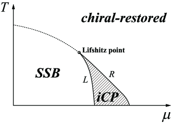
Figure 1: Schematic phase diagram for chiral symmetry breaking in the $(\mu,T)$ plane. The shaded domain enclosed by the left- ($L$-) and right-hand-side ($R$-) boundaries represents the inhomogeneous chiral phase (iCP). The $L$-boundary is of first or second order, depending on the type of iCP dcdw ; nic ; 2d , whereas the $R$-boundary is always of second order, universally. The boundary between the SSB and chiral-restored phases is of second order in the chiral limit (dotted line).

In this paper we elucidate another interesting aspect of the fluctuations near the phase boundary. Starting from the Lifshitz point, iCP is enclosed by the two phase boundaries on the $\mu$-$T$ plane (see Fig. 1): one is the $L$-boundary separating the usual SSB phase and iCP at lower $\mu$, and the other is the $R$-boundary in contact with the chiral-restored phase at larger $\mu$. It has then been shown that the $L$-boundary has different orders and properties of the phase transition, depending on the type of the condensates dcdw ; nic ; 2d , while the $R$-boundary is universal and determined independent of the condensate. Here we look into the phase transition from the side of the chiral-restored phase. Since the order parameter consists of the scalar or pseudoscalar condensate, the effective potential can be written by such a condensate in a symmetric form in the chiral-restored phase. The $R$-boundary may be then found by the analysis of this effective potential, while we cannot see what types of condensates will be realized after the phase transition. In the SSB phase, on the other hand, the effective potential may be written in terms of only the scalar condensate, so that the $L$-boundary can have different predictions. Within the MFA, it has been shown that the chiral-restored phase undergoes the second-order phase transition at the $R$-boundary. We study the nature of the inhomogeneous phase transition around the $R$-boundary by looking into both quantum and thermal fluctuations of quark-antiquark pairs or quark particle-hole pairs (hereinafter collectively called “chiral pairs”) in the chiral-restored phase.

A similar situation also arises in the context of pion condensation in nuclear matter, where nucleon particle-hole pairs are excited mig . In condensed matter physics, it corresponds to the FFLO state in superconductivity, where electron Cooper pairs are excited super . One important common feature prevailing in these phenomena can be seen through the dispersion relation of the fluctuations which has a minimum at a nonzero momentum $|\bm{q}|=q_{c}$ on the two-dimensional sphere in isotropic systems bra ; dyu ; hoh ; fre ; oha , which suggests that the order parameter is spatially modulated after the phase transition. This is qualitatively different from the usual phase transitions, such as homogeneous transitions in superconductivity or those for chiral symmetry breaking, where the spectrum of the fluctuations has a nonzero minimum at $|\bm{q}|=0$. The effect of the fluctuations in the vicinity of the critical point has been studied by Nozière and Schmitt-Rink nsr within the linear (Gaussian) approximation to clarify the BCS-BEC crossover problem. It has been further discussed in the context of a BEC of atoms gri , and also studied to understand a precursor of (color-)superconductivity, known as the pseudogap phenomenon lok ; kit .

A general theory for the inhomogeneous phase transition has been first presented by Brazovskii bra at finite temperature. A similar issue has been discussed by Dyugaev dyu at zero temperature in the context of pion condensation. They have taken into account the interactions among the fluctuations beyond the Gaussian approximation. Unlike the homogeneous phase transition, such a nonlinear effect is now essential. One of the remarkable findings is the change of the order of the phase transition stemming from the fluctuation effects; the second-order phase transition within the MFA is changed to the first-order one (sometimes termed the fluctuation-induced first-order phase transition). This subject has been further studied within the renormalization group approach lin . Also, the Brazovskii theory has been applied to diblock coplymers lei ; fre ; hoh , including its experimental verification bat . However, it seems that the importance of such studies is not fully conceded, e.g., in the discussion of the FFLO state. In the previous work kar , two of the authors (T.T. and T.-G.L.) have presented a heuristic argument about the fluctuation-induced first-order phase transition for the inhomogeneous chiral transition, which we called the Brazovskii-Dyugaev effect. In this paper, extending this work to the general case with $O(N)$ symmetry, we elucidate the particular roles of quantum and thermal fluctuations. We also point out a continuity of the effects of both fluctuations across the phase boundary, by analyzing the behavior of the correlation function attributed to the excitations of the Nambu-Goldstone modes in iCP.

Another purpose of the present paper is to draw one’s attention again to the fluctuation-induced first-order phase transition. Throughout the paper we emphasize some common features for inhomogeneous phase transitions, such as those into the FFLO state in superconductivity. We also discuss some observational implications peculiar to the fluctuation-induced first-order phase transition. Recently, in a B20 compound MnSi which undergoes a fluctuation-induced first-order transition of the Brazovsii type bra , an unequivocal experimental confirmation has been obtained via neutron scattering and thermodynamic observables jan . The first-order character of such a transition may also be expected to be experimentally confirmed for the inhomogeneous chiral transition, e.g., in relativistic heavy-ion collisions.

The paper is organized as follows. In Sec. II, we give a theoretical framework for analyzing the effect of fluctuations around the order parameter in the inhomogeneous chiral transition. After that, in Secs.,III and IV, we discuss the nonlinear effects of fluctuations and the Brazovskii-Dyugaev effect, respectively, before the argument of anomalies in the thermodynamic quantities in Sec. V. Finally, Sec. VI concludes with a summary and remarks.

II Framework

For the following Lagrangian density in the two-flavor Nambu–Jona-Lasinio (NJL) model in the chiral limit, with a quark field for two flavors $\psi$, Pauli matrices in isospin space $\tau$, and a coupling constant $G$,

$${\cal L}={\bar{\psi}}i\partial/\psi+G\left[\left({\bar{\psi}}\psi\right)^{2}+\left({\bar{\psi}}i\gamma_{5}\mbox{\boldmath$\tau$}\psi\right)^{2}\right],$$ (1)

the partition function reads $Z=\int{\cal D}\psi\int{\cal D}{\bar{\psi}}e^{-S}$ with the Euclidean action in imaginary time ($t\rightarrow-i\tau$) being

$$S=-\int_{0}^{\beta}d\tau\int d^{3}\bm{x}\left[{\bar{\psi}}\left(-\gamma^{0}\frac{\partial}{\partial\tau}+i\mbox{\boldmath$\gamma$}\cdot\nabla+\mu\gamma^{0}\right)\psi+G\left[\left({\bar{\psi}}\psi\right)^{2}+\left({\bar{\psi}}i\gamma_{5}\mbox{\boldmath$\tau$}\psi\right)^{2}\right]\right],$$ (2)

where $\beta=1/T$ is the inverse temperature and $\mu$ is the chemical potential. Introducing the auxiliary fields $\phi_{a}=(-2G{\bar{\psi}}\psi,-2G{\bar{\psi}}i\gamma_{5}\mbox{\boldmath$\tau$}\psi)$, one can write the Euclidean partition function as

$$Z = \int{\cal D}\psi\int{\cal D}{\bar{\psi}}\int\prod_{a}{\cal D}\phi_{a}\exp\left[\int_{0}^{\beta}d\tau\int d^{3}\bm{x}\left[{\bar{\psi}}\left(-\gamma^{0}\frac{\partial}{\partial\tau}+i\mbox{\boldmath$\gamma$}\cdot\nabla+\mu\gamma^{0}-(\phi_{0}+i\gamma_{5}\mbox{\boldmath$\tau$}\cdot\mbox{\boldmath$\phi$})\right)\psi-\frac{1}{4G}\phi_{a}^{2}\right]\right]$$ (3)

$$= \int\prod_{a}{\cal D}\phi_{a}e^{-S_{0}},$$

where the effective action is

$$S_{0}=\int_{0}^{\beta}d\tau\int d^{3}\bm{x}\left[\frac{1}{4G}\phi_{a}^{2}\right]-{\rm Tr}{\rm log}\left[-G_{F}^{-1}\right],$$ (4)

with

$$G_{F}^{-1} = -\gamma^{0}\frac{\partial}{\partial\tau}+i\mbox{\boldmath$\gamma$}\cdot\nabla+\mu\gamma^{0}-\left(\phi_{0}+i\gamma_{5}\mbox{\boldmath$\tau$}\cdot\mbox{\boldmath$\phi$}\right)$$ (5)

$$\equiv S_{\beta}^{-1}-\Delta,$$

and $\Delta\equiv(\phi_{0}+i\gamma_{5}\mbox{\boldmath$\tau$}\cdot\mbox{\boldmath$\phi$})$. The inverse of the thermal Green’s function, $S_{\beta}^{-1}$, can be written as $S_{\beta}^{-1}(i\nu_{m},\bm{p})=p/$ with $p_{0}=i\nu_{m}+\mu$ in the frequency and momentum representation, where $\nu_{m}=(2m+1)\pi T$ is the Matsubara frequency for fermions. Thus we find

$$S_{0}(\phi) = \int_{0}^{\beta}d\tau\int d^{3}\bm{x}\left[\frac{1}{4G}\phi_{a}^{2}\right]-{\rm Trlog}[S^{-1}_{\beta}]-\frac{1}{2}{\rm Tr}[\Delta S_{\beta}]^{2}-\frac{1}{4}{\rm Tr}[\Delta S_{\beta}]^{4}+\cdots$$ (6)

$$= S_{f}+\frac{1}{2}T\sum_{n_{1}}\int\frac{d^{3}\bm{q}_{1}}{(2\pi)^{3}}\Gamma_{\rm ps}^{(2)}(i\omega_{n_{1}},\bm{q}_{1})\phi_{a}(i\omega_{n_{1}},\bm{q}_{1})\phi_{a}(-i\omega_{n_{1}},-\bm{q}_{1})$$

$$+\frac{1}{4!}T^{4}\prod_{i=1}^{4}\sum_{n_{i}}\int\frac{d^{3}\bm{q}_{i}}{(2\pi)^{3}}{\hat{\lambda}}(\{i\omega_{n_{i}}\},\{\bm{q}_{i}\})\phi_{a}(i\omega_{n_{1}},\bm{q}_{1})\phi_{a}(i\omega_{n_{2}},\bm{q}_{2})\phi_{b}(i\omega_{n_{3}},\bm{q}_{3})\phi_{b}(i\omega_{n_{4}},\bm{q}_{4})+\cdots,$$

where $\omega_{n}=2\pi nT$ is the Matsubara frequency for bosons and $S_{f}$ is the action for free quarks. Since the component $(\omega_{n}=0$, $|\bm{q}|=q_{c})$ is the relevant degree of freedom, we here approximate the vertex function $\hat{\lambda}$ by the local four-point function ${\hat{\lambda}}(\{i\omega_{n_{i}}\},\{\bm{q}_{i}\})=\lambda(2\pi)^{3}\delta(\bm{q}_{1}+\bm{q}_{2}+\bm{q}_{3}+\bm{q}_{4})\delta(\omega_{n_{1}}+\omega_{n_{2}}+\omega_{n_{3}}+\omega_{n_{4}})$ with a coupling constant $\lambda$. As we shall see later, we must keep the frequency dependence of the composite fields $\phi_{a}$ to extract the correct behavior of the thermodynamic quantities at $T=0$. The above effective action is obviously $SU(2)\times SU(2)\simeq O(4)$ symmetric in the chiral-restored phase. The $q\bar{q}$ polarization function $\Pi^{0}_{\rm ps}(i\omega_{n},\bm{q})$ and the inverse two-point function $\Gamma_{\rm ps}^{(2)}(i\omega_{n},\bm{q})$ are defined, respectively, by

$$\Pi^{0}_{\rm ps}(i\omega_{n},\bm{q})=-N_{f}N_{c}T\sum_{m}\int\frac{d^{3}\bm{p}}{(2\pi)^{3}}{\rm tr}\left[i\gamma_{5}\tau_{3}S_{\beta}(i\omega_{n}+i\nu_{m},\bm{q}+\bm{p})i\gamma_{5}\tau_{3}S_{\beta}(i\nu_{m},\bm{p})\right],$$ (7)

and $$\Gamma_{\rm ps}^{(2)}(i\omega_{n},\bm{q})=\frac{1-2G\Pi^{0}_{\rm ps}(i\omega_{n},\bm{q})}{2G}.$$ (8)

Within the linear approximation for the fluctuations, only the first two terms are sufficient in Eq. (6), without further terms which give the nonlinear effects coming from the mutual interactions of fluctuations, such as the fourth-order term. In the following discussions, however, we keep the terms up to fourth order in $\phi_{a}$, as in a model à la Brazovskii bra ; hoh ; fre .

III Nonlinear effects of fluctuations

We first consider the thermodynamic potential $\Omega=-T{\rm log}Z$ within the linear approximation:

$$\Omega_{\rm LA}=\Omega_{f}+2TV\sum_{n}\int\frac{d^{3}\bm{q}}{(2\pi)^{3}}\ln\left[1-2G\Pi_{\rm ps}^{0}(i\omega_{n},\bm{q})\right],$$ (9)

where $\Omega_{f}$ is the thermodynamic potential for free quarks and $V$ is the volume of the system. This thermodynamic potential corresponds to that obtained by Nozières and Schmitt-Rink nsr for superconductivity. Unlike the homogeneous phase transition, the polarization function has a minimum at $|\bm{q}|=q_{c}\neq 0$, i.e., $\frac{\partial\Pi^{0}_{\rm ps}(0,\bm{q})}{\partial|\bm{q}|}|_{|\bm{q}|=q_{c}}=0$, for the case of the inhomogeneous transition in isotropic systems. Correspondingly, the criterion à la Thouless tho , $1-2G\Pi_{\rm ps}^{0}(i\omega_{n}=0,q_{c})=0$, can be derived as the threshold condition within the MFA. This condition is equivalent to vanishing of the coefficient of the second-order term in Eq. (6).

Next we shall see that the nonlinear effects become essential for the inhomogeneous phase transition, which differs from the usual phase transition. Since the effective action is chiral symmetric, we can choose the thermal average of the pseudoscalar field to be $\beta\Phi(\bm{q})\delta_{n0}=\langle\phi_{3}\rangle$, as an appropriate order parameter for the inhomogeneous chiral transition. Then the thermodynamic potential can be expressed in powers of $\Phi$, after putting $\phi_{a}=\langle\phi_{a}\rangle+\xi_{a}$ and integrating out the fluctuation fields $\xi_{a}$,

$$\Omega = \Omega_{0}+\frac{1}{2!}\prod_{i=1}^{2}\int\frac{d^{3}\bm{q}_{i}}{(2\pi)^{3}}{\bar{\Gamma}}_{\rm ps}^{(2)}(\{\bm{q}_{i}\})\Phi(\bm{q}_{1})\Phi(\bm{q}_{2})$$ (10)

$$+\frac{1}{4!}\prod_{i=1}^{4}\int\frac{d^{3}\bm{q}_{i}}{(2\pi)^{3}}{\bar{\Gamma}}_{\rm ps}^{(4)}(\{\bm{q}_{i}\})\Phi(\bm{q}_{1})\Phi(\bm{q}_{2})\Phi(\bm{q}_{3})\Phi(\bm{q}_{4})$$

$$+\frac{1}{6!}\prod_{i=1}^{6}\int\frac{d^{3}\bm{q}_{i}}{(2\pi)^{3}}{\bar{\Gamma}}_{\rm ps}^{(6)}(\{\bm{q}_{i}\})\Phi(\bm{q}_{1})\Phi(\bm{q}_{2})\Phi(\bm{q}_{3})\Phi(\bm{q}_{4})\Phi(\bm{q}_{5})\Phi(\bm{q}_{6})+\cdots,$$

where each coefficient includes the effects of fluctuations. The first term represents the ring diagrams (bubbles), while the quantities of $\Pi_{\rm ps}^{0}$ are modified by the fluctuations, as we will see below.

III.1 Propagator of a chiral pair fluctuation field

By using the polarization function, we can construct the propagator within the random-phase approximation (RPA). The polarization function defined in Eq. (7) can be written in an apparent form abr ; fet , with the Fermi-Dirac distribution function $f(\epsilon)=(1+e^{\beta\varepsilon})^{-1}$,

$$\Pi_{\rm ps}^{0}(i\omega_{n},\bm{q}) = N_{f}N_{c}\sum_{\bm{p}}\left[(f(|\bm{p}|+\mu)-f(|\bm{p}+\bm{q}|+\mu))\frac{1-\bm{p}\cdot(\bm{p}+\bm{q})/|\bm{p}||\bm{p}+\bm{q}|}{i\omega_{n}+|\bm{p}+\bm{q}|-|\bm{p}|}\right.$$ (11)

$$+(f(|\bm{p}+\bm{q}|-\mu)-1+f(|\bm{p}|+\mu))\frac{1+\bm{p}\cdot(\bm{p}+\bm{q})/|\bm{p}||\bm{p}+\bm{q}|}{i\omega_{n}-|\bm{p}+\bm{q}|-|\bm{p}|}$$

$$+(1-f(|\bm{p}+\bm{q}|+\mu)-f(|\bm{p}|-\mu))\frac{1+\bm{p}\cdot(\bm{p}+\bm{q})/|\bm{p}||\bm{p}+\bm{q}|}{i\omega_{n}+|\bm{p}+\bm{q}|+|\bm{p}|}$$

$$\left.(f(|\bm{p}+\bm{q}|-\mu)-f(|\bm{p}|-\mu))\frac{1-\bm{p}\cdot(\bm{p}+\bm{q})/|\bm{p}||\bm{p}+\bm{q}|}{i\omega_{n}-|\bm{p}+\bm{q}|+|\bm{p}|}\right],$$

which consists of the vacuum contribution, $\Pi_{\rm ps}^{0}(i\omega_{n},\bm{q})|_{(\mu,T)\rightarrow 0}$, and the remaining medium contribution. Here the ultraviolet divergence of the vacuum contribution should be regularized by the proper time regularization (PTR), whose explicit form is described in Ref. kar . Each term in Eq. (11) may be easily understood in terms of particle-antiparticle and particle-hole excitations, where the last term corresponds to the thermal Lindhard function within the nonrelativistic approximation (for details of the derivation, see Appendix A). Note here that the following properties hold: $\Pi_{\rm ps}^{0}(i\omega_{n},\bm{q})=\Pi_{\rm ps}^{0}(-i\omega_{n},\bm{q})$ and $\Pi_{\rm ps}^{0}(i\omega_{n},\bm{q})=\Pi_{\rm ps}^{0}(i\omega_{n},-\bm{q})$.

By the proper analytic continuation $\Pi_{\rm ps}^{0}(i\omega_{n}\rightarrow\omega+i\eta,\bm{q})$, the polarization function can be written as

$$\Pi_{\rm ps}^{0}(i\omega_{n},\bm{q})={\rm Re}\Pi_{\rm ps}^{0}(\omega+i\eta,\bm{q})|_{\omega=i\omega_{n}}+i\,{\rm sign}(\omega_{n}){\rm Im}\Pi_{\rm ps}^{0}(\omega+i\eta,\bm{q})|_{\omega=i\omega_{n}}.$$ (12)

Here we evaluate the imaginary part (for details we refer the reader to Appendix B):

$${\rm Im}\Pi_{\rm ps}^{0}(\omega+i\eta,\bm{q}) =N_{f}N_{c}T\frac{\omega^{2}-q^{2}}{8\pi q}\Big{\{}\ln\left[1+e^{-\beta(q/2+\mu+\omega/2)}\right]-\ln\left[1+e^{-\beta(q/2+\mu-\omega/2)}\right]$$

$$~{}~{}~{}~{}~{}~{}~{}~{}~{}~{}~{}~{}~{}~{}~{}~{}~{}~{}~{}+\ln\left[1+e^{-\beta(q/2-\mu+\omega/2)}\right]-\ln\left[1+e^{-\beta(q/2-\mu-\omega/2)}\right]+\beta\omega\theta(|\omega|-q)\Big{\}},$$ (13)

while we have numerically found it in the previous paper kar .

The Green’s function of chiral pair fluctuation fields, $G_{\rm ps}(i\omega_{n},\bm{q})$, can be then defined by the use of the two-point function (8):

$$G_{\rm ps}(i\omega_{n},\bm{q})\equiv g_{\phi qq}^{-2}[\Gamma_{\rm ps}^{(2)}(i\omega_{n},\bm{q})]^{-1},$$ (14)

where $g_{\phi qq}$ is an effective coupling constant between quarks and a fluctuation field kle . Since the behavior around $|\bm{q}|=q_{c}$ and $\omega_{n}=0$ is important in the vicinity of the phase boundary, we expand it as

$$G_{\rm ps}^{-1}(i\omega_{n},\bm{q})\sim\tau+\gamma\left(|\bm{q}|^{2}-q_{c}^{2}\right)^{2}+\alpha|\omega_{n}|,$$ (15)

where $\tau=G^{-1}_{\rm ps}(0,|\bm{q}|=q_{c})$, $\gamma=\frac{1}{2}d^{2}G^{-1}_{\rm ps}(0,|\bm{q}|=q_{c})/(d|\bm{q}|^{2})^{2}$, and $\alpha=g_{\phi qq}^{2}d{\rm Im}\Pi^{0}_{\rm ps}(\omega=0,|\bm{q}|=q_{c})/d\omega$.

III.2 Thermodynamic potential

Using the effective action with the background field method, we can evaluate the fluctuation effects. Inserting $\phi_{a}=\beta\Phi(\bm{q})\delta_{n0}\delta_{a3}+\xi_{a}$ into Eq. (6), the effective action can be written as

$$S_{0}(\phi_{a})=S_{0}(\Phi)+S_{1}(\Phi,\xi_{a}).$$ (16)

Accordingly, the thermodynamic potential is given by the functional integral:

$$\Omega(\Phi)=TS_{0}(\Phi)-T{\rm log}\int\prod_{a}{\cal D}\xi_{a}{\rm exp}[-S_{1}(\Phi,\xi_{a})].$$ (17)

Each vertex function in Eq. (10) is then given by

$${\bar{\Gamma}}^{(n)}(\bm{q}_{1},\bm{q}_{2},\cdots,\bm{q}_{n})=(2\pi)^{3n}\left.\frac{\delta^{n}\Omega}{\delta\Phi(-\bm{q}_{1})\delta\Phi(-\bm{q}_{2})\cdots\delta\Phi(-\bm{q}_{n})}\right|_{\Phi=0}.$$ (18)

The key equation is the first functional derivative,

$$(2\pi)^{3}\frac{\delta\Omega}{\delta\Phi\left(-\bm{q}_{1}\right)}= ~{}G_{\rm ps}^{-1}\left(0,\bm{q}_{1}\right)\Phi\left(\bm{q}_{1}\right)+\frac{\lambda}{3!}\int\frac{d^{3}\bm{q}_{2}~{}d^{3}\bm{q}_{3}}{(2\pi)^{6}}\Phi\left(\bm{q}_{2}\right)\Phi\left(\bm{q}_{3}\right)\Phi\left(\bm{q}_{1}-\bm{q}_{2}-\bm{q}_{3}\right)$$

$$+\frac{\lambda}{2!}T^{2}\sum_{n}\int\frac{d^{3}\bm{q}_{2}~{}d^{3}\bm{q}_{3}}{(2\pi)^{6}}\left[\langle\xi_{3}\left(i\omega_{n},\bm{q}_{2}\right)\xi_{3}\left(-i\omega_{n},\bm{q}_{3}\right)\rangle_{\xi}+\langle\xi_{0}\left(i\omega_{n},\bm{q}_{2}\right)\xi_{0}\left(-i\omega_{n},\bm{q}_{3}\right)\rangle_{\xi}\right]\Phi\left(\bm{q}_{1}-\bm{q}_{2}-\bm{q}_{3}\right),$$ (19)

where the symbol $\langle\cdots\rangle_{\xi}$ denotes the thermal average, and we have used the following relation: $\langle\xi_{0}\left(i\omega_{n},\bm{q}_{2}\right)\xi_{0}\left(-i\omega_{n},\bm{q}_{3}\right)\rangle_{\xi}=\langle\xi_{1}\left(i\omega_{n},\bm{q}_{2}\right)\xi_{1}\left(-i\omega_{n},\bm{q}_{3}\right)\rangle_{\xi}=\langle\xi_{2}\left(i\omega_{n},\bm{q}_{2}\right)\xi_{2}\left(-i\omega_{n},\bm{q}_{3}\right)\rangle_{\xi}$. In general, the thermal average $\langle\xi(i\omega_{n},\bm{q}_{2})\xi(-i\omega_{n},\bm{q}_{3})\rangle_{\xi}$ has the off-diagonal momentum components, but we can neglect such components as long as the loop integrals are concerned bra . Thus,

$$\langle\xi_{a}(i\omega_{n},\bm{q}_{2})\xi_{a}(-i\omega_{n},\bm{q}_{3})\rangle_{\xi}=\beta(2\pi)^{3}\delta(\bm{q}_{2}+\bm{q}_{3}){\bar{G}}_{a}(i\omega_{n},\bm{q}_{2}).$$ (20)

where $\bar{G}_{a}(i\omega_{n},\bm{q})$ is the self-consistent Green’s function, given by ${\bar{G}}_{a}(i\omega_{n},\bm{q})=[r_{a}+\gamma(|\bm{q}|^{2}-q_{c}^{2})^{2}+\alpha|\omega_{n}|]^{-1}$ with

$$r_{3} = \tau+V^{-1}\frac{\lambda}{2}\int\frac{d^{3}\bm{q}}{(2\pi)^{3}}\Phi\left(\bm{q}\right)\Phi\left(-\bm{q}\right)+\frac{\lambda}{2}T\sum_{n}\int\frac{d^{3}\bm{q}}{(2\pi)^{3}}\left[{\bar{G}_{3}(i\omega_{n},\bm{q})}+{\bar{G}_{0}(i\omega_{n},\bm{q})}\right]$$ (21)

$$\equiv \tau+V^{-1}\frac{\lambda}{2}\int\frac{d^{3}\bm{q}}{(2\pi)^{3}}\Phi\left(\bm{q}\right)\Phi\left(-\bm{q}\right)+\frac{\lambda}{2}\left(I_{1}(r_{3})+I_{1}(r_{0})\right).$$

The integrals $I_{n}$ are defined by

$$I_{n}(r)=T\sum_{k}\int\frac{d^{3}\bm{q}}{(2\pi)^{3}}\left(\frac{\partial^{(n-1)}}{\partial r^{n-1}}\right)\frac{1}{r+\gamma(|\bm{q}|^{2}-q_{c}^{2})^{2}+\alpha|\omega_{k}|},$$ (22)

where the integrals with $n\leq 2$ should be regularized by some regularization methods (see Appendix C for details). Similarly, $r_{0}(=r_{1}=r_{2})$ reads

$$r_{0}=\tau+V^{-1}\frac{\lambda}{6}\int\frac{d^{3}\bm{q}}{(2\pi)^{3}}\Phi\left(\bm{q}\right)\Phi\left(-\bm{q}\right)+\frac{\lambda}{2}\left(I_{1}(r_{3})+I_{1}(r_{0})\right).$$ (23)

While, strictly speaking, there are other two diagrams contributing to $r_{3}$ and $r_{0}$, their contribution can be neglected in the region $r_{3,0}^{1/2}\ll q_{c}$ bra . Using $r_{3}$, Eq. (19) can be rewritten as

$$(2\pi)^{3}\frac{\delta\Omega}{\delta\Phi\left(-\bm{q}_{1}\right)}= \left[r_{3}+\gamma\left(|\bm{q}_{1}|^{2}-q_{c}^{2}\right)^{2}\right]\Phi\left(\bm{q}_{1}\right)-V^{-1}\frac{\lambda}{2!}\Phi\left(\bm{q}_{1}\right)\int\frac{d^{3}\bm{q}_{2}}{(2\pi)^{3}}\Phi\left(\bm{q}_{2}\right)\Phi\left(-\bm{q}_{2}\right)$$

$$+\frac{\lambda}{3!}\int\frac{d^{3}\bm{q}_{2}~{}d^{3}\bm{q}_{3}}{(2\pi)^{6}}\Phi\left(\bm{q}_{2}\right)\Phi\left(\bm{q}_{3}\right)\Phi\left(\bm{q}_{1}-\bm{q}_{2}-\bm{q}_{3}\right).$$ (24)

Thus, $\Gamma^{(1)}$ is obviously vanished as should be expected. Subsequent derivatives of $\Omega$ give the even-order vertex functions. Note here that $r_{a}$ is a functional of $\Phi$ and their derivatives satisfy the following equations:

$$\frac{\delta r_{3}}{\delta\Phi(-\bm{q}_{2})} = \frac{(2\pi)^{-3}V^{-1}\lambda\Phi(\bm{q}_{2})}{1-\frac{\lambda}{2}I_{2}(r_{3})}+\frac{\frac{\lambda}{2}I_{2}(r_{0})}{1-\frac{\lambda}{2}I_{2}(r_{3})}\cdot\frac{\delta r_{0}}{\delta\Phi(-\bm{q}_{2})},$$

$$\text{and}\quad\frac{\delta r_{0}}{\delta\Phi(-\bm{q}_{2})} = \frac{(2\pi)^{-3}V^{-1}\frac{\lambda}{3}\Phi(\bm{q}_{2})}{1-\frac{\lambda}{2}I_{2}(r_{0})}+\frac{\frac{\lambda}{2}I_{2}(r_{3})}{1-\frac{\lambda}{2}I_{2}(r_{0})}\cdot\frac{\delta r_{3}}{\delta\Phi(-\bm{q}_{2})}.$$ (25)

The second-order vertex function thus reads

$${\bar{\Gamma}}^{(2)}(\bm{q}_{1},\bm{q}_{2})=(2\pi)^{3}\delta(\bm{q}_{1}+\bm{q}_{2})(\tau_{R}+\gamma(|\bm{q}|^{2}-q_{c}^{2})^{2}),$$ (26)

where $\tau_{R}=r_{3}(\Phi=0)=r_{0}(\Phi=0)$. Likewise, the fourth-order vertex function is

$${\bar{\Gamma}}^{(4)}(\{\bm{q}_{i}\})=(2\pi)^{3}\lambda\left[\delta(\bm{q}_{1}+\bm{q}_{2}+\bm{q}_{3}+\bm{q}_{4})+(2\pi)^{3}V^{-1}\frac{\frac{2\lambda}{3}I_{2}(\tau_{R})}{1-\lambda I_{2}(\tau_{R})}\left[\delta(\bm{q}_{1}+\bm{q}_{2})\delta(\bm{q}_{3}+\bm{q}_{4})+2~{}{\rm permutations}\right]\right].$$ (27)

IV Brazovskii-Dyugaev effect

IV.1 Fluctuation-induced first-order phase transition

First, we consider the second-order term (26). If $\tau_{R}$ becomes zero, it should be a signal of the second-order phase transition. From Eq. (21), $\tau_{R}$ satisfies

$$\tau_{R} = \tau+\lambda I_{1}(\tau_{R}),$$

$$\text{with}\quad\tau~{} = \tau_{R}-\frac{\lambda T}{2\pi^{2}}\int_{\tau_{R}/\Lambda^{2}}^{\infty}{ds}\left[\frac{\tau_{R}^{1/2}}{2}\left(\frac{\pi}{(4\gamma q_{c}^{2}s)^{3}}\right)^{1/2}+\tau_{R}^{-1/2}\left(\frac{\pi q_{c}^{2}}{4\gamma s}\right)\right]e^{-s}{\rm coth}\left(\frac{\alpha\pi Ts}{\tau_{R}}\right).$$ (28)

Looking into the behavior around $\tau_{R}=0$, we find that

$$\tau \simeq \tau_{R}-\frac{\lambda Tq_{c}}{4\pi\gamma^{1/2}\tau_{R}^{1/2}}~{}~{}~{}{\rm for}~{}~{}T\neq 0,$$ (29)

$$\text{while}\quad\tau \simeq \tau_{R}-\frac{\lambda\Lambda^{3}}{48\alpha\pi^{5/2}\gamma^{3/2}q_{c}^{3}}~{}~{}~{}{\rm for}~{}~{}T=0.$$ (30)

This is due to the singularity of $G_{\rm ps}^{R}(i\omega_{n},\bm{q})$ on the sphere $|\bm{q}|=q_{c}$, which is a common feature for inhomogeneous phase transitions in isotropic systems bra ; dyu ; hoh ; fre ; oha . From Eq. (29) and Fig. 2, we can see that $\tau$ diverges at $\tau_{R}=0$ and $\tau_{R}$ is always positive for all range of $\tau$, which implies that the phase transition is prohibited at finite temperature. On the other hand, there is no divergence at zero temperature. In addition, the point $\tau_{R}=0$ at $T=0$ is somewhat shifted fromthe point $\tau=0$. The difference of $T\neq 0$ and $T=0$ can be easily understood from the fact that the lowest Matsubara frequency is dominant and the leading behavior (29) can be obtained by putting $\omega_{n}=0$ into the integral $I_{2}$. Thus we can observe that there takes place a kind of dimensional reduction from $1+3$ to $0+3$ dimensions at $T\neq 0$. It would be interesting to see a similarity to the Coleman-Mermin-Wagner theorem cmw , which claims that the lower critical dimension is $1+2$ for thermal fluctuations wen . In the case of $T=0$, the imaginary part in $\bar{G}_{\rm ps}$ becomes important to lead to no divergent behavior; quantum fluctuations are gentle and only shifts the critical point.

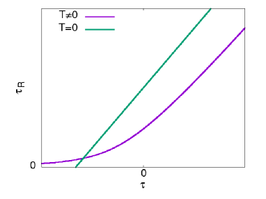
Figure 2: The $\tau$ dependences of $\tau_{R}$ at $T\neq 0$ (purple curve) and $T=0$ (green line). $\tau_{R}$ always takes positive values when $T\neq 0$, while, when $T=0$, it vanishes at $\tau=-\frac{\lambda\Lambda^{3}}{48\alpha\pi^{5/2}\gamma^{3/2}q_{c}^{3}}$.

The above considerations are insufficient for the possibility of the phase transition due to the only consideration for the second-order phase transition. Next, we shall introduce the fourth-order and sixth-order vertex functions to see whether the system undergoes the first-order phase transition. The sign change of the fourth-order vertex function by fluctuations has been first shown by Brazovskii  at $T\neq 0$ and Dyugaev at $T=0$. The integral $I_{2}(\tau_{R})$ in $\bar{\Gamma}^{(4)}$ which will be seen in Eq. (36) can be evaluated as

$$I_{2}(\tau_{R})=-\frac{T}{2\pi^{2}}\int_{0}^{\infty}ds\left[\frac{1}{2}\left(\frac{\pi}{(4\gamma q_{c}^{2})^{3}s}\right)^{1/2}\tau_{R}^{-1/2}+\left(\frac{\pi q_{c}^{2}s}{4\gamma}\right)^{1/2}\tau_{R}^{-3/2}\right]e^{-s}{\rm coth}\left(\frac{\alpha\pi Ts}{\tau_{R}}\right).$$ (31)

Looking into the behavior around $\tau_{R}=0$, we find that

$$I_{2}(\tau_{R}) \simeq -\frac{Tq_{c}}{8\pi\gamma^{1/2}}\tau_{R}^{-3/2}~{}~{}~{}{\rm for}~{}~{}T\neq 0,$$ (32)

$$\text{while}\quad I_{2}(\tau_{R}) \simeq -\frac{q_{c}}{4\alpha\pi^{2}\gamma^{1/2}}\tau_{R}^{-1/2}~{}~{}~{}{\rm for}~{}~{}T=0.$$ (33)

This result shows that the effects of fluctuations lead to the divergence of the integral $I_{2}$ near the phase boundary. Unlike $\tau_{R}$, quantum fluctuations also give rise to a singular behavior, while it is less drastic than thermal fluctuations. These features can be understood as for the case of $\tau_{R}$. The expression (27) is physically given by summing up the “dangerous diagrams,” which are composed of bubbles of the renormalized propagator in the chiral-restored phase,

$$G_{\rm ps}^{R}(i\omega_{n},\bm{q}) = {\bar{G}}_{\rm ps}(i\omega_{n},\bm{q};\tau=\tau_{R})$$ (34)

$$= \frac{1}{\tau_{R}+\gamma(|\bm{q}|^{2}-q_{c}^{2})^{2}+\alpha|\omega_{n}|},$$

and also represent the long-range interaction among chiral pair fluctuations,

$$L(\bm{k})=T\sum_{n}\int\frac{d^{3}\bm{q}}{(2\pi)^{3}}G_{\rm ps}^{R}(i\omega_{n},\bm{q})G_{\rm ps}^{R}(-i\omega_{n},\bm{k}-\bm{q}).$$ (35)

We can easily see that $L(\bm{k})$ becomes the most singular and $L(\bm{k})\rightarrow-I_{2}(\tau_{R})$ as $k\rightarrow 0$: the singularities in $G^{R}_{\rm ps}(i\omega_{n},\bm{q})$ and $G^{R}_{\rm ps}(-i\omega_{n},\bm{k}-\bm{q})$ come closer as $k\rightarrow 0$ to make the integral divergent. Finally, we find

$${\bar{\Gamma}^{(4)}}=(2\pi)^{3}\lambda\frac{1+\frac{\lambda}{3}I_{2}(\tau_{R})}{1-\lambda I_{2}(\tau_{R})}\delta(\bm{q}_{1}+\bm{q}_{2}+\bm{q}_{3}+\bm{q}_{4}),$$ (36)

assuming the form of the condensate as $\Phi=\Delta{\rm sin}(q_{c}z)$. Hence, the sign of ${\bar{\Gamma}^{(4)}}$ is changed at the point, $1+\frac{\lambda}{3}I_{2}(\tau_{R})=0$, which suggests that the phase transition is of first order, i.e., the fluctuation-induced first-order phase transition.

In the above discussion, the $O(4)$ model including four fluctuation fields is considered. We next expand the discussion to the $O(N)$ model for theoretical interests. For arbitrary $N$, Eqs. (21) and (23) are recast into

$$r_{3} = \tau+V^{-1}\frac{\lambda}{2}\int\frac{d^{3}\bm{q}}{(2\pi)^{3}}\Phi\left(\bm{q}\right)\Phi\left(-\bm{q}\right)+\frac{\lambda}{2}\left(I_{1}(r_{3})+\frac{N-1}{3}I_{1}(r_{0})\right),$$ (37)

$$r_{0} = \tau+V^{-1}\frac{\lambda}{6}\int\frac{d^{3}\bm{q}}{(2\pi)^{3}}\Phi\left(\bm{q}\right)\Phi\left(-\bm{q}\right)+\frac{\lambda}{2}\left(I_{1}(r_{3})+\frac{N-1}{3}I_{1}(r_{0})\right).$$ (38)

Consequently, $\bar{\Gamma}^{(4)}$ is modified as follows:

$${\bar{\Gamma}^{(4)}}=(2\pi)^{3}\lambda\frac{1+\frac{10-N}{18}\lambda I_{2}(\tau_{R})}{1-\frac{N+2}{6}\lambda I_{2}(\tau_{R})}\delta(\bm{q}_{1}+\bm{q}_{2}+\bm{q}_{3}+\bm{q}_{4}).$$ (39)

In the case of $N=1$, the previous result obtained in kar is reproduced, and the result for $N=4$ coincides with Eq. (36). In the case of $N\geq 10$, on the other hand, the fluctuation-induced first-order phase transition does not occur because $\bar{\Gamma}^{(4)}$ never becomes negative.

IV.2 Continuity of the roles of fluctuations across the phase boundary

Here we discuss a similar feature of the fluctuations in iCP. We have found that the effects of fluctuations are remarkable for the phase transition, and the role of thermal fluctuations is more profound than that of quantum fluctuations. On the other hand, it has been shown that the fluctuations in iCP are important to cause the instability of one-dimensional structures at finite temperature lee : the scalar or pseudoscalar correlation function, $f_{a}(\bm{r})=\langle\phi_{a}(\bm{r})\phi_{a}(0)\rangle$ where $\phi_{a}$ denote the quark bilinear fields in scalar or pseudoscalar channel (i.e., $\phi_{0}={\bar{\psi}}\psi$ and $\phi_{i}={\bar{\psi}}i\gamma_{5}\tau_{i}\psi$), algebraically decays at large distances due to the low-energy Nambu-Goldstone excitations. It is in accord with the Landau-Peierls theorem lan ; pei . For definiteness, we here consider inhomogeneous chiral condensates of the dual chiral density wave (DCDW) type. There appear three Naumbu-Goldstone modes ($\beta_{i}$) with the anisotropic dispersion $\omega_{i}^{2}=A_{i}k_{z}^{2}+B_{i}k_{\perp}^{4}$. In the case of $T=0$, we find

$$\langle\beta_{i}(\bm{r})^{2}\rangle_{T=0}=c_{i}\int\frac{d^{4}k}{(2\pi)^{4}}\frac{1}{k_{0}^{2}+A_{i}k_{z}^{2}+B_{i}k_{\perp}^{4}},$$ (40)

where $k_{z}$ is the momentum in the direction parallel to the wave vector of the modulation, while $k_{\perp}$ is that in the directions normal to the modulation. Here the coefficients $c_{i}$, $A_{i}$, and $B_{i}$ can be evaluated within chiral effective models nic . The above integral is convergent in the infrared region. In the case of $T\neq 0$, on the other hand, we find

$$\langle\beta_{i}(\bm{r})^{2}\rangle_{T\neq 0} = c_{i}T\sum_{\omega_{n}}\int_{-\infty}^{\infty}\frac{dk_{z}}{2\pi}\int_{l^{-1}_{\perp}}^{\Lambda_{\perp}}\frac{d^{2}\bm{k}_{\perp}}{(2\pi)^{2}}\frac{1}{\omega_{n}^{2}+A_{i}k_{z}^{2}+B_{i}k_{\perp}^{4}},$$ (41)

$$\sim \frac{c_{i}T}{8\pi\sqrt{A_{i}B_{i}}}\ln(\Lambda_{\perp}l_{\perp}),$$

which is divergent in the infrared region $(l_{\perp}^{-1}\rightarrow 0)$. The most dominant contribution comes from the lowest Matsubara frequency $\omega_{n}=0$,

$$\langle\beta_{i}(\bm{r})^{2}\rangle_{T\neq 0}\sim c_{i}T\int_{-\infty}^{\infty}\frac{dk_{z}}{2\pi}\int_{l^{-1}_{\perp}}^{\Lambda_{\perp}}\frac{d^{2}\bm{k}_{\perp}}{(2\pi)^{2}}\frac{1}{A_{i}k_{z}^{2}+B_{i}k_{\perp}^{4}},$$ (42)

and exhibits an infrared singularity due to the effective dimensional reduction. This implies that thermal fluctuations play a more important role in the infrared singularity than quantum ones. In this way, we can see the similar features to our results obtained in the previous subsection.

The stability of the DCDW phase an also be understood in the same way. Here the correlation function of the order parameter $\phi_{3}$ takes the form lee ; hid ,

$$\langle\phi_{3}(z)\phi_{3}(0)\rangle\sim e^{-\frac{1}{2}\langle\left[\beta_{3}(z)-\beta_{3}(0)\right]^{2}\rangle}.$$ (43)

From this, we find that for $T=0$,

$$\langle\left[\beta_{3}(z)-\beta_{3}(0)\right]^{2}\rangle_{T=0} = c_{i}\int\frac{d^{4}k}{(2\pi)^{4}}\frac{1-e^{ik_{z}z}}{k_{0}^{2}+A_{i}k_{z}^{2}+B_{i}k_{\perp}^{4}}$$ (44)

$$\sim \frac{c_{i}}{16\pi\sqrt{A_{i}B_{i}}}\Lambda~{}~{}{\rm for~{}large}~{}|z|,$$

while for $T\neq 0$,

$$\langle\left[\beta_{3}(z)-\beta_{3}(0)\right]^{2}\rangle_{T\neq 0} = c_{i}T\sum_{\omega_{n}}\int\frac{d^{3}\bm{k}}{(2\pi)^{3}}\frac{1-e^{ik_{z}z}}{\omega_{n}^{2}+A_{i}k_{z}^{2}+B_{i}k_{\perp}^{4}}$$ (45)

$$\sim \frac{c_{i}T}{8\pi\sqrt{A_{i}B_{i}}}\ln\left(A_{i}^{-1/2}\Lambda|z|\right)~{}~{}{\rm for~{}large}~{}|z|,$$

where the latter logarithmically diverges in the limit $|z|\rightarrow\infty$, and $\Lambda$ is an ultraviolet cutoff. For details we refer the reader to Appendix D. Similarly, the same results can be obtained for other order parameters. Here thermal fluctuations are still important for the same reason. Therefore, we can conclude that the correlation function algebraically decays only for $T\neq 0$ and the DCDW phase shows the feature of quasi-long range order lee (see also hid for RKC). These results may suggest some continuity of the roles of fluctuations before and after the phase transition, as far as the one-dimensional modulation is concerned.

V Anomalies in the thermodynamic quantities

It is well known that fluctuations affect the thermodynamic quantities around the phase boundary. Anomalies in various susceptibilities (the second derivatives of the thermodynamic potential) are characteristic features near the critical point of the second-order phase transition; the specific-heat anomaly, $C_{v}\sim(T-T_{c})^{-1/2}$, has been shown due to fluctuations at the critical temperature $T_{c}$ of superconductivity, while there is generated a finite discontinuity within the MFA. In the context of the usual chiral transition, the divergence of the quark number susceptibility, $\partial N/\partial\mu$, has been discussed fuj .

The singular behavior of the propagator gives rise to new types of anomalies in the thermodynamic quantities for the inhomogeneous phase transition. In the context of the FFLO state in superconductivity, Ohashi have indicated the divergence of the electron number due to the fluctuation oha , where $N\sim\tau^{-1/2}$ within the linear approximation, which means that the first derivative of the thermodynamic potential becomes singular. As we have seen in the previous section, $\tau$ is renormalized to keep it to be positive definite by the non-linear effects, and the singularity mentioned above can not be observed. However, its remnant should be observed. Thus, the fluctuation-induced first-order transition is characterized by the discontinuity and singular behavior of the first derivative.

In the following, we shall discuss the quark number and the entropy for the inhomogeneous chiral transition. In the chiral-restored phase ($\Phi=0$), the thermodynamic potential is given by

$$\Omega(\Phi=0)=\Omega_{f}-2TV\sum_{n}\int\frac{d^{3}\bm{q}}{(2\pi)^{3}}\ln\left(G_{\rm ps}^{R}(i\omega_{n},\bm{q})\right),$$ (46)

which is a simple generalization of Eq. (9) with a replacement of $\tau$ by $\tau_{R}$. The quark number density can be written as

$$n=n_{f}+2T\sum_{n}\int\frac{d^{3}\bm{q}}{(2\pi)^{3}}G_{\rm ps}^{R}(i\omega_{n},\bm{q})\frac{\partial}{\partial\mu}{\bar{\Pi}}^{0}_{\rm ps}(i\omega_{n},\bm{q}),$$ (47)

where

$$n_{f}=\frac{N_{c}N_{f}}{\pi^{2}}\int_{0}^{\infty}p^{2}dp\left(f(p-\mu)-f(p+\mu)\right).$$ (48)

Using Eq. (34) and $I_{1}$ derived from Appendix C, the fluctuation effects then can be seen separately:

$$n \sim n_{f}+\frac{1}{\tau_{R}^{1/2}}\frac{N_{f}N_{c}q_{c}}{8\pi^{3}\gamma^{1/2}}\int_{-\infty}^{\infty}pdp\frac{1}{[e^{\beta(p+\mu)/2}+e^{-\beta(p+\mu)/2}]^{2}}\left(4+\frac{q_{c}}{p}\ln\left|\frac{2p-q_{c}}{2p+q_{c}}\right|\right)~{}~{}~{}{\rm for}~{}~{}~{}T\neq 0,$$ (49)

$$\sim n_{f}-\frac{N_{f}N_{c}\Lambda^{3}}{96\pi^{9/2}\alpha\gamma^{3/2}q_{c}^{3}}\left(4\mu+q_{c}\ln\left|\frac{2\mu-q_{c}}{2\mu+q_{c}}\right|\right)~{}~{}~{}{\rm for}~{}~{}~{}T=0,$$

as the leading contribution. Thus we can see a singular behavior at $T\neq 0$, while at $T=0$ only a finite gap is produced. A similar divergence ($\propto\tau_{R}^{-1/2}$) is also observed in the entropy. The entropy density is given by

$$s=s_{f}-2\sum_{n}\int\frac{d^{3}\bm{q}}{(2\pi)^{3}}\ln G_{\rm ps}^{R}(i\omega,\bm{q})+2T\sum_{n}\int\frac{d^{3}\bm{q}}{(2\pi)^{3}}G_{\rm ps}^{R}(i\omega,\bm{q})\frac{\partial}{\partial T}{\bar{\Pi}}^{0}_{\rm ps}(i\omega_{n},\bm{q}),$$ (50)

where

$$s_{f}=\frac{2N_{f}N_{c}}{\pi^{2}}\int_{0}^{\infty}pdp\left[(2p-\mu)\ln(1+e^{-\beta(p-\mu)})+(2p+\mu)\ln(1+e^{-\beta(p-\mu)})\right].$$ (51)

The second term gives a minor contribution ($\propto\ln\tau_{R}$), while the leading contribution comes from the third term,

$$s\sim s_{f}-\frac{1}{\tau_{R}^{1/2}}\frac{N_{f}N_{c}q_{c}}{8\pi^{3}\gamma^{1/2}T}\int_{-\infty}^{\infty}dp\frac{p(p+\mu)}{\left[e^{\beta(p+\mu)/2}+e^{-\beta(p+\mu)/2}\right]^{2}}\left(4+\frac{q_{c}}{p}\ln\left|\frac{2p-q_{c}}{2p+q_{c}}\right|\right),$$ (52)

around the phase boundary. Such a anomalous behavior may be reflected in the particle production during relativistic heavy-ion collisions, if the system crosses the phase boundary. Here it would be worth mentioning that the entropy anomaly may also be a signal of the FFLO state.

VI Summary and concluding remarks

We have discussed the effects of chiral pair fluctuations on the inhomogeneous chiral transition by extending the previous work. Also, we have taken into account the non-linear effects of chiral-pair fluctuations in a systematic way beyond the linear approximation. Eventually, we have elucidated the salient roles of quantum and thermal fluctuations separately; the latter is more drastic than the former due to the dimensional reduction, but both lead to the fluctuation-induced first-order phase transition. The curvature parameter $\tau$ is renormalized by the fluctuation effects to be positive definite at $T\neq 0$, while for $T=0$ it is mildly shifted from the one within MFA. Thus, we have observed that the second-order phase transition is prohibited by thermal fluctuations. More importantly, the dangerous diagrams composed of the bubbles of two fluctuation Green’s function become essential and change the sign of the fourth-order vertex function for both the $T=0$ and $T\neq 0$ cases. The sign of the sixth-order vertex function can be shown to be positive definite, and thus we can clearly see the first-order phase transition. These features are brought about by the unique behavior of the dispersion of chiral pair fluctuations, and also common in any inhomogeneous phase transition.

It should be worth mentioning that the behavior of the vertex functions has been also studied by solving the flow equations within the renormalization group approach, and in addition the findings with the perturbative approach have been confirmed for diblock copolymers hoh . The renormalization group is somewhat different from the usual treatment due to the existence of the special point $q_{c}$ in momentum space, but can be formulated in the similar way to the work by Shankar sha for fermion many-body systems, where the Fermi momentum corresponds to $q_{c}$. Since our formalism is very much similar to theirs, one may expect that our findings are also confirmed by the renormalization group approach. This is left for a future work.

The first derivative of the thermodynamic potential exhibits a singular behavior through the momentum integral, since the dispersion of chiral pair fluctuations has a minimum on the sphere $|\bm{q}|=q_{c}$. To figure out such a singular behavior, we have evaluated the number density and entropy density, with the result that the fluctuation-induced first-order phase transition can be characterized by the discontinuity and singular behavior of the first derivatives.

Throughout the paper, we have discussed the properties of the $R$-boundary. As for the $L$-boundary, it has been shown that it should be of first order in the case of DCDW, while of second order in the case of RKC. Therefore, it would be interesting to apply our argument to the $R$-boundary of RKC, where the number susceptibility has been suggested to be divergent within the MFA car .

In this paper we have been concerned the effects of fluctuations of the order parameters. The singular feature of the propagator of a fluctuation field may also affect the quark propagator lok ; kit ; the self-energy of quarks should exhibit another anomalous behavior near the phase boundary.

Finally it would be worth mentioning that our formalism to treat the non-linear effects of fluctuations may also be applied to other cases, such as the FFLO state in superconductivity lee2 ; the Cooper pair fluctuations are composed of the particle-particle ladder diagram instead, but the dispersion relation has a similar feature discussed here. Accordingly, the entropy anomaly may be a possible evidence for the phase transition.

Appendix A Thermal Lindhard function

In the nonrelativistic limit, we consider the particle-hole polarization function (the Lindhard function at $T\neq 0$),

$$\chi(q) = T\sum_{\bm{p}}G\left(p+\frac{q}{2}\right)G\left(p-\frac{q}{2}\right)$$ (53)

$$= \sum_{\bm{p}}\frac{f(\varepsilon_{+})-f(\varepsilon_{-})}{\varepsilon_{+}-\varepsilon_{-}+i\omega_{n}},$$

where $\varepsilon_{\pm}=\frac{(\bm{p}\pm\bm{q}/2)^{2}}{2m}-\mu$. This can be also obtained from the imaginary part of the polarization function in the relativistic case after the analytic continuation ($i\omega_{n}\rightarrow\omega+i\eta$). The imaginary part takes the form

$${\rm Im}\chi(\bm{q},\omega+i\eta) =-\pi\sum_{\bm{p}}\left[f(\epsilon_{+})-f(\epsilon_{-})\right]\delta(\epsilon_{+}-\epsilon_{-}+\omega)$$

$$=-\frac{1}{4\pi}\int_{0}^{\infty}p^{2}dp\int_{-1}^{1}dx\left[f\left(\zeta_{p}+\frac{pq}{2m}x\right)-f\left(\zeta_{p}-\frac{pq}{2m}x\right)\right]\delta\left(\frac{pq}{m}x+\omega\right),$$ (54)

where $\zeta_{p}=\frac{p^{2}}{2m}+\frac{q^{2}}{8m}-\mu$. Considering the argument of the delta function, we find

$${\rm Im}\chi(\bm{q},\omega+i\eta) =-\frac{m}{4\pi q}\int_{0}^{\infty}pdp\left[f\left(\zeta_{p}-\frac{\omega}{2}\right)-f\left(\zeta_{p}+\frac{\omega}{2}\right)\right]\theta\left(-\frac{pq}{m}<\omega<\frac{pq}{m}\right)$$

$$=-\frac{m^{2}T}{4\pi q}\left[\ln\left\{1+e^{-\beta\left(\frac{m\omega^{2}}{2q^{2}}+\frac{q^{2}}{8m}-\mu-\frac{\omega}{2}\right)}\right\}-\ln\left\{1+e^{-\beta\left(\frac{m\omega^{2}}{2q^{2}}+\frac{q^{2}}{8m}-\mu+\frac{\omega}{2}\right)}\right\}\right].$$ (55)

Appendix B Imaginary part of the polarization function

The imaginary part of $\Pi_{\rm ps}^{0}(\bm{q},\omega+i\eta)$ is given by

$${\rm Im}\Pi_{\rm ps}^{0}(\bm{q},\omega+i\eta) =-N_{f}N_{c}\pi\int\frac{d^{3}\bm{p}}{(2\pi)^{3}}\bigg{\{}\left[f(|\bm{p}|+\mu)-f(|\bm{p}+\bm{q}|+\mu)\right]\left[1-\frac{\bm{p}\cdot(\bm{p}+\bm{q})}{|\bm{p}||\bm{p}+\bm{q}|}\right]\delta(\omega+|\bm{p}+\bm{q}|-|\bm{p}|)$$

$$~{}~{}~{}~{}~{}~{}~{}~{}~{}~{}~{}~{}~{}~{}~{}~{}~{}~{}+\left[f(|\bm{p}+\bm{q}|-\mu)-f(|\bm{p}|-\mu)\right]\left[1-\frac{\bm{p}\cdot(\bm{p}+\bm{q})}{|\bm{p}||\bm{p}+\bm{q}|}\right]\delta(\omega-|\bm{p}+\bm{q}|+|\bm{p}|)$$

$$~{}~{}~{}~{}~{}~{}~{}~{}~{}~{}~{}~{}~{}~{}~{}~{}~{}~{}+\left[f(|\bm{p}+\bm{q}|-\mu)-1+f(|\bm{p}|+\mu)\right]\left[1+\frac{\bm{p}\cdot(\bm{p}+\bm{q})}{|\bm{p}||\bm{p}+\bm{q}|}\right]\delta(\omega-|\bm{p}+\bm{q}|-|\bm{p}|)$$

$$~{}~{}~{}~{}~{}~{}~{}~{}~{}~{}~{}~{}~{}~{}~{}~{}~{}~{}+\left[1-f(|\bm{p}+\bm{q}|+\mu)-f(|\bm{p}|-\mu)\right]\left[1+\frac{\bm{p}\cdot(\bm{p}+\bm{q})}{|\bm{p}||\bm{p}+\bm{q}|}\right]\delta(\omega+|\bm{p}+\bm{q}|+|\bm{p}|)\bigg{\}}.$$ (56)

Each delta function is evaluated as

$$\delta(\omega+|\bm{p}+\bm{q}|-|\bm{p}|) =\frac{p-\omega}{pq}\delta\left(x-\frac{\omega^{2}-2p\omega-q^{2}}{2pq}\right)\theta(p-\omega),$$ (57)

$$\delta(\omega-|\bm{p}+\bm{q}|+|\bm{p}|) =\frac{p+\omega}{pq}\delta\left(x-\frac{\omega^{2}+2p\omega-q^{2}}{2pq}\right)\theta(p+\omega),$$ (58)

$$\delta(\omega-|\bm{p}+\bm{q}|-|\bm{p}|) =\frac{-p+\omega}{pq}\delta\left(x-\frac{\omega^{2}-2p\omega-q^{2}}{2pq}\right)\theta(-p+\omega),$$ (59)

$$\delta(\omega+|\bm{p}+\bm{q}|+|\bm{p}|) =\frac{-p-\omega}{pq}\delta\left(x-\frac{\omega^{2}+2p\omega-q^{2}}{2pq}\right)\theta(-p-\omega),$$ (60)

where $x=\cos\theta$. Considering the argument of the delta function, we find

$${\rm Im}\Pi_{\rm ps}^{0}(\bm{q},\omega+i\eta) =N_{f}N_{c}\frac{\omega^{2}-q^{2}}{8\pi q}\int_{0}^{\infty}dp\bigg{\{}\left[f(p+\mu)-f(p+\mu-\omega)\right]\theta(p-\omega)\theta\left(-1<\frac{\omega^{2}-2p\omega-q^{2}}{2pq}<1\right)$$

$$~{}~{}~{}~{}~{}~{}~{}~{}~{}~{}~{}~{}~{}~{}~{}~{}~{}~{}+\left[f(p-\mu+\omega)-f(p-\mu)\right]\theta(p+\omega)\theta\left(-1<\frac{\omega^{2}+2p\omega-q^{2}}{2pq}<1\right)$$

$$~{}~{}~{}~{}~{}~{}~{}~{}~{}~{}~{}~{}~{}~{}~{}~{}~{}~{}-\left[-f(p+\mu-\omega)+f(p+\mu)\right]\theta(-p+\omega)\theta\left(-1<\frac{\omega^{2}-2p\omega-q^{2}}{2pq}<1\right)$$

$$~{}~{}~{}~{}~{}~{}~{}~{}~{}~{}~{}~{}~{}~{}~{}~{}~{}~{}-\left[f(p-\mu+\omega)-f(p-\mu)\right]\theta(-p-\omega)\theta\left(-1<\frac{\omega^{2}+2p\omega-q^{2}}{2pq}<1\right)\bigg{\}}.$$ (61)

Therefore,

$${\rm Im}\Pi_{\rm ps}^{0}(\bm{q},\omega+i\eta) =N_{f}N_{c}T\frac{\omega^{2}-q^{2}}{8\pi q}\Big{\{}\ln\left[1+e^{-\beta(q/2+\mu+\omega/2)}\right]-\ln\left[1+e^{-\beta(q/2+\mu-\omega/2)}\right]$$

$$~{}~{}~{}~{}~{}~{}~{}~{}~{}~{}~{}+\ln\left[1+e^{-\beta(q/2-\mu+\omega/2)}\right]-\ln\left[1+e^{-\beta(q/2-\mu-\omega/2)}\right]+\beta\omega\theta(|\omega|-q)\Big{\}}.$$ (62)

Appendix C Integrals $I_{n}$

We evaluate the integrals $I_{n}$ by using the proper time formalism,

$$I_{n}(r)=(-1)^{n-1}T\sum_{m}\int\frac{d^{3}\bm{q}}{(2\pi)^{3}}\int_{0}^{\infty}ds\,s^{n-1}e^{-s\left[r+\gamma\left(|\bm{q}|^{2}-q_{c}^{2}\right)^{2}+\alpha|\omega_{m}|\right]}.$$ (63)

The Matsubara frequency can be summed up as follows:

$$I_{n}(r)=(-1)^{n-1}T\int\frac{d^{3}\bm{q}}{(2\pi)^{3}}\int_{0}^{\infty}ds\,s^{n-1}e^{-s\left[r+\gamma\left(|\bm{q}|^{2}-q_{c}^{2}\right)^{2}\right]}\coth(\alpha\pi Ts).$$ (64)

If $r$ is sufficiently small, the main region contributed to the integral is $|\bm{q}|\sim q_{c}$. Therefore, the integral can be approximated as

$$I_{n}(r) \simeq\frac{(-1)^{n-1}T}{4\pi^{2}}\int_{-\infty}^{\infty}q^{2}dq\int_{0}^{\infty}ds\,s^{n-1}\left\{e^{-s\left[r+4\gamma q_{c}^{2}\left(q-q_{c}\right)^{2}\right]}+e^{-s\left[r+4\gamma q_{c}^{2}\left(q+q_{c}\right)^{2}\right]}\right\}\coth(\alpha\pi Ts)$$

$$=\frac{(-1)^{n-1}T}{2\pi^{2}}\int_{0}^{\infty}ds\left(\frac{1}{2}\sqrt{\frac{\pi}{(4\gamma q_{c}^{2}s)^{3}}}+\sqrt{\frac{\pi q_{c}^{2}}{4\gamma s}}\right)s^{n-1}e^{-sr}\coth(a_{1}\pi Ts).$$ (65)

When $n=1,2$, the proper time regularization should be introduced because the integrals have an ultraviolet divergence. However, the reading contribution is not affected by the cutoff at $r\sim 0$, except for $n=1$ at $T=0$.

Appendix D Correlation function in the DCDW phase

In the case of $T=0$, the correlation function takes the form

$$\langle\left[\beta_{i}(z)-\beta_{i}(0)\right]^{2}\rangle_{T=0} = c_{i}\int\frac{d^{4}k}{(2\pi)^{4}}\frac{1-e^{ik_{z}z}}{k_{0}^{2}+A_{i}k_{z}^{2}+B_{i}k_{\perp}^{4}}$$ (66)

$$= \frac{c_{i}}{16\pi^{3}\sqrt{B_{i}}}\int^{\infty}_{-\infty}dk_{0}\int^{\infty}_{-\infty}dk_{z}\int^{\infty}_{0}dx\frac{1-e^{ik_{z}z}}{k_{0}^{2}+A_{i}k_{z}^{2}+x^{2}},$$

where $x=\sqrt{B_{i}}k_{\perp}^{2}$. Furthermore, putting $y=\sqrt{x^{2}+k_{0}^{2}}$, we can obtain

$$\langle\left[\beta_{i}(z)-\beta_{i}(0)\right]^{2}\rangle_{T=0} = \frac{c_{i}}{16\pi^{2}\sqrt{B_{i}}}\int^{\infty}_{-\infty}dk_{z}\int^{\infty}_{0}ydy\frac{1-e^{ik_{z}z}}{y^{2}+A_{i}k_{z}^{2}}$$ (67)

$$= \frac{c_{i}}{16\pi^{2}\sqrt{A_{i}B_{i}}}\int^{\Lambda}_{0}dy\left(1-e^{-A^{-1/2}_{i}y|z|}\right)$$

$$\sim \frac{c_{i}}{16\pi\sqrt{A_{i}B_{i}}}\Lambda~{}~{}~{}{\rm for~{}large}~{}|z|,$$

where the ultraviolet cutoff $\Lambda$ is inserted. In the case of $T\neq 0$, on the other hand, the leading contribution comes from the lowest Matsubara frequency,

$$\langle\left[\beta_{i}(z)-\beta_{i}(0)\right]^{2}\rangle_{T\neq 0} \sim c_{i}T\int\frac{d^{3}\bm{k}}{(2\pi)^{3}}\frac{1-e^{ik_{z}z}}{A_{i}k_{z}^{2}+B_{i}k_{\perp}^{4}}$$ (68)

$$= \frac{c_{i}T}{8\pi^{2}\sqrt{B_{i}}}\int^{\infty}_{-\infty}dk_{z}\int^{\infty}_{0}dx\frac{1-e^{ik_{z}z}}{A_{i}k_{z}^{2}+x^{2}}$$

$$= \frac{c_{i}T}{8\pi\sqrt{A_{i}B_{i}}}\int^{\Lambda}_{0}dx\frac{1-e^{-A_{i}^{-1/2}x|z|}}{x}.$$

Here we insert the convergence factor,

$$\langle\left[\beta_{i}(z)-\beta_{i}(0)\right]^{2}\rangle_{T\neq 0} \sim \lim_{\epsilon\to+0}\frac{c_{i}T}{8\pi\sqrt{A_{i}B_{i}}}\int^{A_{i}^{-1/2}\Lambda|z|}_{0}dx\frac{1-e^{-x}}{x^{1-\epsilon}}$$ (69)

$$= \lim_{\epsilon\to+0}\frac{c_{i}T}{8\pi\sqrt{A_{i}B_{i}}}\left[\frac{1}{\epsilon}\left(A_{i}^{-1/2}\Lambda|z|\right)^{\epsilon}-\Gamma(\epsilon)+\Gamma(\epsilon,A_{i}^{-1/2}\Lambda|z|)\right]$$

$$\sim \frac{c_{i}T}{8\pi\sqrt{A_{i}B_{i}}}\ln\left(A_{i}^{-1/2}\Lambda|z|\right)~{}~{}~{}{\rm for~{}large}~{}|z|.$$

References

- (1) K. Fukushima and T. Hatsuda, Rept. Prog. Phys. 74, 014001 (2011); K. Fukushima and C. Sasaki, Prog. Part. Nucl. Phys. 72, 99 (2013).
- (2) D. V. Deryagin, D. Yu. Grigoriev, and V.A. Rubakov, Int. J. Mod. Phys. A 7, 659 (1992); E. Shuster and D. T. Son, Nucl. Phys. B 573, 434 (2000); B.-Y. Park, M. Rho, A. Wirzba, and I. Zahed, Phys. Rev. D 62, 034015 (2000); R. Rapp, E. Shuryak, and I. Zahed, Phys. Rev. D 63 034008 (2001).
- (3) T. Tatsumi and E. Nakano, hep-ph/0408294; E. Nakano and T. Tatsumi, Phys. Rev. D 71, 114006 (2005).
- (4) D. Nickel, Phys. Rev. Lett. 103, 072301 (2009); Phys. Rev. D 80, 074025 (2009).
- (5) M. Buballa and S. Carignano, Prog. Part. Nucl. Phys. 81, 39 (2015).
- (6) I. E. Frolov, V. Ch. Zhukovsky, and K. G. Klimenko, Phys. Rev. D 82, 076002 (2010).
- (7) T. Tatsumi, K. Nishiyama, and S. Karasawa, Phys. Lett. B 743, 66 (2015).
- (8) R. Yoshiike, K. Nishiyama, and T. Tatsumi, Phys. Lett. B 751, 123 (2015).
- (9) R. Yoshiike and T. Tatsumi, Phys. Rev. D 92, 116009 (2015).
- (10) T.-G. Lee, E. Nakano, Y. Tsue, T. Tatsumi, and B. Friman, Phys. Rev. D 92, 034024 (2015).
- (11) Y. Hidaka, K. Kamikado, T. Kanazawa, and T. Noumi, Phys. Rev. D 92, 034003 (2015).
- (12) L.D. Landau and E.M. Lifshitz, Statistical Physics, (Pergamon Press, Oxford, 1969).
- (13) R. E. Peierls, Quantum Theory of Solids (Oxford University Press, 1955).
- (14) P. G. de Gennes and J. Prost, The physics of liquid crystals (Oxford University Press, 1974); P. M. Chaikin and T. C. Lubensky, Principles of condensed matter physics (Cambridge Univ Press, 2000); W. H. de Jeu, B. I. Ostrovskii, and A. N. Shalaginov, Rev. Mod. Phys. 75, 181 (2003).
- (15) H. Shimahara, J. Phys. Soc. Jpn. 67, 1872 (1998); H. Shimahara, Physica B: Condensed Matter 259, 492 (1999).
- (16) L. Radzihovsky and A. Vishwanath, Phys. Rev. Lett. 103, 010404 (2009); L. Radzihovsky, Phys. Rev. A 84, 023611 (2011); Physica C: Superconductivity 481, 189 (2012).
- (17) T. Giamarchi and P. Le Doussal, Phys. Rev. Lett. 72, 1530 (1994); Phys. Rev. B 52, 1242 (1995); T. Nattermann and S. Scheidl, Adv. Phys. 49, 607 (2000).
- (18) G. Baym, B. Friman, and G. Grinstein, Nucl. Phys. B 210, 193 (1982).
- (19) V. Berezinskii, Sov. Phys. JETP 32, 493 (1971); J. M. Kosterlitz and D. J. Thouless, J. Phys. C 6, 1181 (1973).
- (20) Z. Hadzibabic, P. Krüger, M. Cheneau, B. Battelier, and J. Dalibard, Nature 441, 1118 (2006).
- (21) P. A. Murthy, I. Boettcher, L. Bayha, M. Holzmann, D. Kedar, M. Neidig, M. G. Ries, A. N. Wenz, G. Zurn, and S. Jochim, Phys. Rev. Lett. 115, 010401 (2015).
- (22) W. H. Nitsche, N. Y. Kim, G. Roumpos, C. Schneider, M. Kamp, S. Höfling, A. Forchel, and Y. Yamamoto, Phys. Rev. B 90, 205430 (2014).
- (23) S. Carignano and M. Buballa, Phys. Rev. D 86, 074018 (2012).
- (24) A. B. Migdal, Rev. Mod. Phys. 50 (1978) 107; A .B. Migdal, E. E. Saperstein, M. A. Troitsky, and D. N. Voskresensky, Phys. Rep. 192, 179 (1990).
- (25) P. Fulde and R. A. Ferrel, Phys. Rev. 135, A550 (1964); A. I. Larkin and Y. N. Ovchinnikov, Sov. Phys. JETP 20, 762 (1965); R. Casalbuoni and G. Nardulli, Rev. Mod. Phys. 76, 263 (2004); Y. Liao, A. S. C. Rittner, T. Paprotta, W. Li, G. B. Partridge, R. G. Hulet, S. K. Baur, and E. J. Mueller, Nature 467, 567 (2010).
- (26) S. A. Brazovskii, Sov. Phys. JETP 41, 85 (1975).
- (27) A. M. Dyugaev, Sov. Phys. JETP Lett. 22, 83 (1975).
- (28) P. C. Hohenberg and J. B. Swift, Phys. Rev. E 52, 1828 (1995).
- (29) G. H. Fredkickson and K. Binder, J. Chem.Phys. 91, 7265 (1989).
- (30) Y. Ohashi, J. Phys. Soc. Jpn. 71, 2625 (2002).
- (31) P. Nozières and S. Schmitt-Rink, J. Low Temp. Phys. 59, 195 (1985).
- (32) Y. Ohashi and A. Griffin, Phys. Rev. Lett. 89, 130402 (2002); Phys. Rev. A 67, 063612 (2003).
- (33) V. M. Loktev, R. M. Quick, and S. G. Sharapov, Phys. Rep. 349, 1 (2001).
- (34) M. Kitazawa, T. Koide, T. Kunihiro, and Y. Nemoto, Phys. Rev. D 65 (2002) 091504; 70, 056003 (2004).
- (35) D. D. Ling, B. Friman, and G. Grinstein, Phys. Rev. B 24, 2718 (1981).
- (36) L. Leibler, Macromolecules 13, 1602 (1980).
- (37) F. S. Bates, J. H. Rosedale, and G. H. Fredickson, J. Chem. Phys. 92, 6255 (1990).
- (38) S. Karasawa, T.-G. Lee, and T. Tatsumi, Prog. Theor. Exp. Phys. 2016, 043D02 (2016).
- (39) B. I. Halperin, T. C. Lubensky, and S. Ma, Phys. Rev. Lett. 32, 292 (1974).
- (40) P. Bak, S. Krinsky, and D. Mukamel, Phys. Rev. Lett. 36, 52 (1976).
- (41) K. Binder, Rep. Prog. Phys. 50, 783 (1997).
- (42) M. Janoschek, M. Garst, A. Bauer, P. Krautscheid, R. Georgii, P. Böni, and C. Pfleiderer, Phys. Rev. B 87, 134407 (2013).
- (43) D. J. Thouless, Ann. Phys. 10, 553 (1960).
- (44) A. A. Abrikosov, L. P. Gorkov, and I. E. Dzyaloshinskii, Methods of Quantum Field Theory in Statistical Physics (Prentice-Hall, Inc., Englewood Cliffs, New Jersey, 1963).
- (45) A. L. Fetter and J. L. Walecka, Quantum Theory of Many-Particle Systems (McGraw-Hill, , New York, 1971).
- (46) S. P. Klevansky, Rev. Mod. Phys. 64, 649 (1992).
- (47) S. R. Coleman, Commun. Math. Phys. 31, 259 (1973); N. D. Mermin and H. Wagner, Phys. Rev. Lett. 17, 1133(1966); P. C. Hohenberg, Phys. Rev. 158, 383 (1967).
- (48) X.-G. Wen, Quantum Field Theory of Many-Body Systems (Oxford University Press, 2004).
- (49) H. Kleinert, Phys. Lett. B 102, 1 (1981).
- (50) L. Radzihovsky, Phys. Rev. A84, 023611 (2011).
- (51) H. Fujii, Phys. Rev. D 67, 094018 (2003); H. Fujii and M. Ohtani, Phys. Rev. D 70, 014016 (2004).
- (52) R. Shankar, Rev. Mod. Phys. 66, 129 (1994).
- (53) S. Carignano, D. Nickel and M. Buballa, Phys. Rev. D 82, 054009 (2010).
- (54) T.-G. Lee, R. Yoshiike and T. Tatsumi, in preparation.