Direct numerical simulation of particulate flows with an overset grid method

Abstract

We evaluate an efficient overset grid method for two-dimensional and three-dimensional particulate flows for small numbers of particles at finite Reynolds number. The rigid particles are discretised using moving overset grids overlaid on a Cartesian background grid. This allows for strongly-enforced boundary conditions and local grid refinement at particle surfaces, thereby accurately capturing the viscous boundary layer at modest computational cost. The incompressible Navier–Stokes equations are solved with a fractional-step scheme which is second-order-accurate in space and time, while the fluid–solid coupling is achieved with a partitioned approach including multiple sub-iterations to increase stability for light, rigid bodies. Through a series of benchmark studies we demonstrate the accuracy and efficiency of this approach compared to other boundary conformal and static grid methods in the literature. In particular, we find that fully resolving boundary layers at particle surfaces is crucial to obtain accurate solutions to many common test cases. With our approach we are able to compute accurate solutions using as little as one third the number of grid points as uniform grid computations in the literature. A detailed convergence study shows a 13-fold decrease in CPU time over a uniform grid test case whilst maintaining comparable solution accuracy.

1 Introduction

Flows of finite-sized particles in viscous fluids are common to many industrial as well as natural processes, such as primary cementing in the oil and gas industry [52] and blood flow [3]. Being so ubiquitous, particulate-flow problems span a large range of material and flow properties. Of interest to this work are flows of an incompressible Newtonian fluid with rigid, spherical (circular) particles of finite Reynolds number, where the Reynolds number describes the relative strength of inertial to viscous forces.

Approximate solution methods have been applied to both high and low particle Reynolds number flow regimes, where by neglecting viscous or inertial contributions, respectively, the equations of motion can be linearised and solved with powerful mathematical tools; see [62, 44, 13] for examples in both flow regimes. It is the intermediate flow regime, where such approximations are not valid, that the full incompressible Navier–Stokes equations must be solved. Direct numerical simulation methods designed for such intermediate Reynolds number flow regimes broadly fit into two categories: those methods that use a static grid that is unaligned with the particle boundaries, and those that use boundary-conforming grids. Below we give a brief overview of these two classes of methods and their application to particulate flow problems.

Arbitrary Lagrangian Eulerian (ALE) methods were developed for deforming boundary problems as a response to the difficulties encountered when using fully Lagrangian schemes in problems with large amounts of circulation, see for example, [11]. The ALE method belongs to the class of boundary conformal methods, to which the boundary integral method (only applicable to inviscid, irrotational flow) and the overset grids method belong. The semi-discrete, viz. finite element in space and finite difference in time, method of Hughes et al. [37] has proved popular with general fluid structure interaction (FSI) problems and has been continually developed over the last few decades. In this ALE approach, nodal velocities explicitly enter the convective terms of the momentum equations allowing the underlying grid to distort with the moving boundary, while an Eulerian description can be used in regions of large circulation. Hu et al. [35] used an ALE method with a combined fluid–solid formulation to simulate pairs of spheres interacting in Newtonian and visco-elastic liquids, and 2D sedimentation simulations of 90 circular particles.

This ALE method can be considered a special case of the deforming spatial domain or stabilised space-time (DSD/SST) method developed by Tezduyar et al. [66], where a finite element formulation is used both in space and time. By extending the finite element formulation in time any grid deformation is automatically accounted for [66]. To avoid turning a three dimensional problem into a four dimensional problem, courtesy of the time dimension, a discontinuous-in-time space-time finite element formulation of the problem is solved for one space-time “slab” at a time.

Both the conventional ALE and DSD/SST methods use unstructured grids to explicitly represent the particle surface. Unstructured grids allow for complex surfaces to be represented but are generally not amenable to fast elliptic solvers, such as geometric multigrid. The distortion of the underlying grid inevitably causes elements to become increasingly skewed. Highly skewed elements can often cause problems relating to accuracy and stability, requiring a new grid to be computed on to which the solution is then projected. Both the regridding and projection steps are costly procedures and are the main drawbacks of ALE and DSD/SST type methods [27]. Particulate flow simulations generally encounter large deformations, requiring frequent regridding.

Various approaches have been developed to improve the quality of the deformed grid. Johnson and Tezduyar [38], for example, used the equations of linear elasticity to govern the deformation of the grid for their particulate flow simulations. The grid distortion was controlled through a stiffness parameter, effectively weighting distortion towards larger elements. This preserved smaller elements in the surface regions that are important to the accuracy of the overall solution. By promoting less important elements, i.e. those far away from the particle surfaces, to distort more easily, regridding is reduced since the grid quality is, potentially, preserved for longer. However, this comes at the cost of solving an additional partial differential equation for the grid deformation.

Due to the complexities and costs of the unstructured regridding associated with boundary-conforming grid methods, the static grid methods have gained favour with many researchers for approaching FSI problems.

Static grid methods can be split into two categories based on the treatment of the solid–fluid interface: diffuse interface and sharp interface methods. An efficient class of diffuse interface methods is the immersed boundary (IB) method. The original IB method of Peskin [59] was developed to study flow patterns around heart valves. The entire computational domain is represented by a Cartesian grid and the interface is represented by a collection of massless Lagrangian points. The velocity of these Lagrangian points is used to compute the stress on the elastic interface through a constitutive relation, such as Hooke’s law. This singular force distribution is transmitted from the Lagrangian interface points to the Eulerian fluid through a forcing term in the momentum equation. The information transfer is facilitated by a discrete Dirac delta function, smoothly spreading the force from the Lagrangian to the Eulerian grid. Aside from inherent stability benefits, this approach is attractive because only the right-hand side of the momentum equation is affected, so no changes to the underlying solver are required. Assuming constant density across the entire domain also allows fast Poisson solvers to be used without modification [41].

Directly applying Peskin’s original IB method to rigid boundary problems is not straightforward because the constitutive relation for the elastic boundary is generally not well behaved in the rigid limit [50]. Uhlmann [67] used the direct forcing formulation of Mohd-Yusof [51] whilst retaining the smooth information transfer between Lagrangian and Eulerian grid points. Direct forcing methods use a virtual forcing term determined by the difference between the desired interface velocities and the velocities interpolated from the underlying Eulerian grid. Uhlmann proposed evaluating the forcing term at the Lagrangian interface points before smoothly transferring it to Eulerian grid points in order to reduce spatial oscillations common to direct forcing methods. With this direct forcing IB method, Uhlmann and Doychev [68] performed sedimentation simulations with $\mathcal{O}(10^{4})$ spherical particles in tri-periodic domains.

Kempe and Fröhlich [41] modified the interpolation and spreading procedure of [67], greatly improving on the Courant–Friedrichs–Lewy (CFL) time step restriction and the stability for light bodies, achieving particle–fluid density ratios as low as $\rho_{r}=0.3$ for spherical particles. With this IB method Vowinckel et al. [69] investigated turbulent channel flow with mobile beds consisting of $\mathcal{O}(10^{4})$ spherical particles.

Glowinski et al. [26] developed a distributed Lagrange multiplier/fictitious domain method (DLM/FD) reminiscent of Peskin’s IB method using the principle of variational inequality in a finite element context. A combined variational formulation of the fluid-solid coupling was used—similar to that of [34]—but the rigidity was enforced in the particle subdomains through Lagrange multipliers, thereby allowing the governing equations to be solved on stationary grids. The original DLM/FD method imposed velocity on the particle subdomain. Patankar et al. [57] imposed the deformation-rate tensor instead in order to simplify treatment for irregularly shaped particles, while Wachs [70] used this formulation in conjunction with a discrete element method to develop an improved collision mechanism for irregularly shaped bodies.

The smoothing intrinsic to diffuse interface methods reduces the solution accuracy in the immediate vicinity of the interface. This can be addressed through increased grid resolution, but at the cost of greatly increased calculation size given the grid uniformity. This problem is particularly severe in high Reynolds number flows, where the viscous boundary layer is thin. One popular way to improve accuracy at the interface is through the use of sharp interface methods, which generally reconstruct the solution near the interface, thereby enforcing the boundary conditions strongly. Fadlun et al. [21] developed a hybrid approach that borrowed on the momentum forcing approach of [59] but with the goal of enforcing boundary conditions exactly. Fadlun et al. [21] used the direct forcing formulation of [51], but imposed boundary conditions by directly modifying the coefficients of the linear system rather than explicitly calculating the forcing. This was done in order to avoid solving an implicit system for the forcing, which came about because of the implicit treatment of the viscous terms in their fractional step time advancement scheme [21]. In effect, this is equivalent to applying momentum forcing inside the fluid domain, leading to problems with moving grids when previously “solid” grid points are converted to “fluid” points. Yang and Balaras [73] demonstrated that unphysical information carried by a previously solid point into the flow field makes the evaluation of the right-hand side of the momentum equation in the fractional step algorithm problematic. They developed a “field extension” strategy, whereby the velocity and pressure fields are extended into the solid phase at the end or beginning of each sub-step. Borazjani et al. [12], developed a sharp interface method based on front-tracking for general curvilinear background grids that can handle an arbitrary number of bodies in three dimensions. Added-mass effects were treated with sub-iterations and an Aitken acceleration technique. Recently, Yang and Stern [74] improved on the field extension strategy through the introduction of temporary non-inertial reference frames attached to the solid phases. This is based on the fluid–solid coupling strategy of Kim and Choi [43] and allows the velocity coupling to be done in a non-iterative fashion. Crucially, [74] only use the non-inertial reference frame for the forcing, solving the flow field on the inertial reference frame and thereby allowing for an arbitrary number of solid phases. By allowing non-iterative methods to be used for the forcing and rigid-body motion calculations, [74] improved the performance by up to an order of magnitude. However, such field extension strategies reduce the sharpness of the immersed boundary, diminishing the advantage over diffuse methods [63].

Flow reconstruction based sharp interface methods suffer from force oscillations in moving boundary problems [48]. This is caused by the instantaneous role reversal of a grid point from an interpolation to a discrete Navier–Stokes point, and vice versa, when crossed by the boundary. This role reversal involves an immediate change in computational stencil, causing a temporal discontinuity that even the field extension of [73] does not address [48]. Seo and Mittal [63] explored the source of the temporal discontinuity in their study using a cut-cell sharp interface method and were able to reduce the oscillations by roughly an order of magnitude through improved geometric mass conservation near the interface.

Much recent effort has been focused on static grid methods for particulate flow, owing to the high efficiency of such methods and the desire to simulate engineering flows containing huge numbers of particles. Broadly speaking, boundary conformal methods can offer superior accuracy near the solid/fluid interface but may be inefficient for problems with large spatial deformations due to the costs associated with regridding at each time step. On the other hand, static grid methods—which can be highly efficient— have difficulty resolving the boundary layers near particles and may require very fine grids or adaptive grid refinement to obtain accurate results [71].

In this work we will evaluate the overset grid, or Chimera grid, method for viscous particulate flow. Overset grid methods have been widely used for problems with moving geometries. They were recognised early on to be a useful technique for treating rigid moving bodies, such as aircraft store separation [19], and have subsequently been applied to many other moving-grid aerodynamic applications, see for example [49, 33, 75, 15, 16, 46]. English et al. [20] present a novel overset grid approach using a Voronoi grid to link Cartesian overset grids. This differs to the method used here, where interpolation stencils are directly substituted into the coefficient matrix and solid boundaries are represented using curvilinear grids. The basic approach of moving overset grids used in this article was developed for high-speed compressible and reactive flows by [33] and included the support for adaptive grid refinement. The deforming composite grid (DCG) approach was developed in [6] for treating deforming bodies with overset grids, and a partitioned scheme was developed for light deforming bodies that was stable without sub-iterations. A method to overcome the added-mass instability with compressible flows and rigid bodies was developed in [9]. More recently, stable partitioned schemes for incompressible flows and deforming solids have been developed [7, 8, 47] and extended to non-linear solids [5].

The method described in this paper retains much of the efficiency of static structured grid methods whilst still allowing for sharp representation of solid boundaries. The overset grid method can be seen as a bridge between the static grid methods such as IBM and boundary conformal grid methods; the curvilinear particle grids allow for higher than first-order accuracy and boundary conditions to be implemented strongly, while grid connectivity with the static Cartesian background grid is only locally updated. Since the grid connectivity is only updated locally, the regridding procedure is less costly and complex than for unstructured body conformal methods, such as ALE. Local grid refinement allows boundary layers to be fully resolved without appreciably affecting the total grid point count. This is in contrast with general static grid methods where the solver efficiency is offset by the unfavourable scaling associated with uniform grids, making large fully resolved simulations very costly [71]. For these reasons, we evaluate the suitability of the method for fully resolved simulations of incompressible fluid flow with rigid particles. Note that the scheme described here is implemented in the Cgins solver that is available as part of the Overture framework of codes (overtureFramework.org). Although past papers have described the use of Cgins for bodies undergoing specified motions (e.g. [14]), the discussion here of the algorithm involving freely-moving rigid-bodies is new.

In section 2 the overset grid method is summarised, before stating the mathematical formulation in section 3. These equations are discretised in space and time in section 4 and 5, respectively, while section 6 presents the fluid–solid coupling methodology. A grid convergence study is performed in section 7.1 using a representative test case to determine appropriate spatial resolutions for the wake structures captured by the background grid, and boundary layer captured by the particle grid. Following this, validation cases in both two and three space dimensions are presented, comparing against published experimental and numerical results. The results of our evaluation are summarised in section 8, along with an outlook towards future work.

2 Overset grids

The method of overset grids (also called overlapping, overlaid or Chimera grids) bridges the stationary and boundary conformal grid methods. A complex domain is represented by multiple body-fitted curvilinear grids that are allowed to overlap, as shown in Fig. 1. Overset grids bring flexibility to grid generation since component grids are not required to align along block boundaries. This flexibility allows component grids to be added in a relatively independent manner, requiring only local changes to grid connectivity.

A composite grid $\boldsymbol{\mathcal{G}}$ consists of logically rectangular component grids $\boldsymbol{\mathcal{G}}_{k}$, with $k=1,2,\dots N_{g}$. As illustrated in Fig. 1 the grid points of $\boldsymbol{\mathcal{G}}$ are classified as interior points, boundary points, interpolation points and exterior or un-used points. The algorithm for generating a composite grid from a collection of component grids is intricate; a detailed description is beyond the remit of this work and so it will be only briefly discussed, with the intention of showing why the method of overset grids is appropriate for particulate flow problems. The interested reader is referred to [17] and [29] for a full description of the algorithm and implementation.

Figure 1: Left: an overlapping grid consisting of two structured curvilinear component grids, $\boldsymbol{x}=\boldsymbol{\mathcal{G}}_{1}(\boldsymbol{r})$ and $\boldsymbol{x}=\boldsymbol{\mathcal{G}}_{2}(\boldsymbol{r})$. Middle and right: component grids for the square and annular grids in the unit square parameter space $\boldsymbol{r}$. Grid points are classified as discretisation points, interpolation points or unused points. Ghost points are used to apply boundary conditions.

When moving grids are used, as is the case in particulate flow problems where each particle is represented by a separate component grid, the relative position of overset grids changes continuously. As a result, overlapping connectivity information, i.e. Chimera holes (regions of exterior points in the overset component grids) and interpolation points, must be recomputed at every time-step. Crucially, this is cheaper than complete grid regeneration and the required connectivity information recomputation can be locally confined to those grids affected by the moving grid.

Values of the solution at interpolation points are determined by standard tensor-product Lagrange-interpolation. We use quadratic interpolation (three-point stencil in each direction) for the results in this paper, as required for second-order accuracy [17]. This interpolation is not locally conservative. Locally conservative interpolation on overset grids is possible [18] but has not been found necessary in our experience. Corrections to ensure global conservation are also possible and have been shown to have advantages, see for example [64].

3 Governing equations

Incompressible flow is governed by the Navier–Stokes equations,

$$\frac{\partial\boldsymbol{u}}{\partial t}+(\boldsymbol{u}\cdot\nabla)\boldsymbol{u} =-\frac{1}{\rho}\nabla p+\nu\nabla^{2}\boldsymbol{u}+\boldsymbol{f},$$

$$\nabla\cdot\boldsymbol{u} =0,$$

where $\boldsymbol{u}$ is the vector of Cartesian components of the velocity $u_{i}$, $p$ the pressure field, $\rho$ the fluid density, and $\nu=\mu/\rho$ the kinematic viscosity. For discretising the equations on a moving grid (on an overset grid some grids are static while others are attached to, and move with the body), we make a change of dependent variables $\boldsymbol{x}$ and $t$ to a frame that moves with the grid. As a result, on moving domains, the governing equations transform to

$$\frac{\partial\boldsymbol{u}}{\partial t}+((\boldsymbol{u}-\boldsymbol{w}))\cdot\nabla\boldsymbol{u} =-\frac{1}{\rho}\nabla p+\nu\nabla^{2}\boldsymbol{u}+\boldsymbol{f},$$ (1)

$$\nabla\cdot\boldsymbol{u} =0,$$ (2)

where $\boldsymbol{w}$ is the velocity of a point attached to the moving domain. The partial derivative in time in the moving frame, as appearing in (1), is therefore the derivative in time when keeping the spatial location fixed to a point that is attached to the moving domain. We solve an alternative formulation of system (1)-(2). A pressure Poisson equation is derived by taking the divergence of the momentum equation (1) and using (2). The resulting velocity–pressure formulation of the initial-boundary value problem is

$$\frac{\partial\boldsymbol{u}}{\partial t}+({(\boldsymbol{u}-\boldsymbol{w})}\cdot{\nabla})\boldsymbol{u}+\frac{1}{\rho}{\nabla}p-\nu{\nabla}^{2}\boldsymbol{u}-\boldsymbol{f} =0,\qquad\qquad\forall\boldsymbol{x}\in\Omega,$$ (3)

$$\mathcal{J}({\nabla}\boldsymbol{u})+\frac{1}{\rho}{\nabla}^{2}p-{\nabla}\cdot\boldsymbol{f} =0,\qquad\qquad\forall\boldsymbol{x}\in\Omega,$$ (4)

$${B}(\boldsymbol{u},p) =\boldsymbol{0},\qquad\qquad\forall\boldsymbol{x}\in\partial\Omega,$$ (5)

$${\nabla}\cdot\boldsymbol{u} =0,\qquad\qquad\forall\boldsymbol{x}\in\partial\Omega,$$ (6)

$$\boldsymbol{u}(\boldsymbol{x},0) =\boldsymbol{u}_{0}(\boldsymbol{x}),\qquad\text{at}\quad t=0,$$ (7)

where $\mathcal{J}(\nabla\boldsymbol{u})\equiv\nabla\boldsymbol{u}:\nabla\boldsymbol{u}$ and $\Omega$ denotes the fluid domain in $n_{d}$ space dimensions. There are $n_{d}$ primary boundary conditions, denoted by $B(\boldsymbol{u},p)=\boldsymbol{0}$. The velocity–pressure formulation requires an additional boundary condition for the pressure. Here, the velocity divergence (6) is applied as the boundary condition on the pressure, making the velocity–pressure formulation equivalent to the velocity–divergence formulation [28]. For the second-order accurate scheme used here, boundary conditions are required to determine $\boldsymbol{u}$ and $p$ at a line of fictitious (ghost) points outside the domain boundary. Some of the numerical boundary conditions are compatibility conditions, derived by applying the momentum and pressure equations on the boundary.

The motion of a rigid body immersed in the fluid is governed by the Newton–Euler equations,

$$\frac{\mathrm{d}\boldsymbol{x}_{b}}{\mathrm{d}t}=\boldsymbol{v}_{b},\quad m_{b}\frac{\mathrm{d}\boldsymbol{v}_{b}}{\mathrm{d}t}=\boldsymbol{F},\quad A\frac{\mathrm{d}\boldsymbol{\omega}}{\mathrm{d}t}=-\boldsymbol{\omega}\times A\boldsymbol{\omega}+\boldsymbol{T},\quad\frac{\mathrm{d}\boldsymbol{e}_{i}}{\mathrm{d}t}=\boldsymbol{\omega}\times\boldsymbol{e}_{i}.$$

Here $\boldsymbol{x}_{b}(t)$ and $\boldsymbol{v}_{b}(t)$ are the position and velocity of the centre of mass, respectively, $m_{b}$ is the mass of the body, $\boldsymbol{\omega}$ is the angular velocity, $A$ is the moment of inertia matrix, $\boldsymbol{e}_{i}$ are the principal axes of inertia, $\boldsymbol{F}(t)$ is the applied force, and $\boldsymbol{T}(t)$ is the applied torque about the centre of mass of the body. The principal axes of inertia are integrated over time to find the rotation matrix which is used to update positions, velocities and acceleration of points attached to the body surface.

The force and torque on the body are determined from both body forces, such as gravity, and hydrodynamic forces arising from the stresses exerted by the fluid on the body surface, $\Gamma$,

$$\boldsymbol{F}=\int_{\Gamma}(-p\boldsymbol{n}+\boldsymbol{\tau}\cdot\boldsymbol{n})\;\mathrm{d}s+\boldsymbol{f}_{b},\qquad\boldsymbol{T}=\int_{\Gamma}(\boldsymbol{x}-\boldsymbol{x}_{b})\times(-p\boldsymbol{n}+\boldsymbol{\tau}\cdot\boldsymbol{n})\;\mathrm{d}s+\boldsymbol{t}_{b},$$

where $\boldsymbol{x}$ is a point on $\Gamma$, $\boldsymbol{\tau}=\mu(\nabla\boldsymbol{u}+(\nabla\boldsymbol{u})^{T})$ is the viscous stress tensor, $\boldsymbol{n}$ is the unit normal vector to the body surface (outward pointing from the fluid domain), $\boldsymbol{f}_{b}$ is any external body force and $\boldsymbol{t}_{b}$ is any external body torque.

4 Spatial discretisation

The equations of the velocity-pressure formulation are discretised to second-order accuracy in space using finite difference methods on overset grids, see [28] and [32]. An overset grid consists of logically rectangular grids that cover a grid region and overlap where they coincide. The solutions between adjacent grids are connected via interpolation conditions. Each component grid (numbered $k=1,2,\dots,N_{g}$) is associated with a transformation $\boldsymbol{d}_{k}:\mathbb{R}^{3}\rightarrow\mathbb{R}^{3}$ from the unit square, with coordinates denoted by $\boldsymbol{r}=(r_{1},r_{2},r_{3})$, into physical space, $\boldsymbol{x}=(x_{1},x_{2},x_{3})$, and denoted by $\boldsymbol{d}_{k}(\boldsymbol{r},t)=\boldsymbol{x}(\boldsymbol{r},t)$, which allows for body fitted grids of non-rectangular shapes. Consider solving the equations in three space dimensions on a square component grid $\boldsymbol{\mathcal{G}}_{k}$, with grid spacing $h_{m}=1/N_{m}$, for a positive integer $N_{m}$:

$$\boldsymbol{\mathcal{G}}_{k}=\{\boldsymbol{x}_{\boldsymbol{i},k}~{}|~{}\boldsymbol{i}=(i_{1},i_{2},i_{3}),~{}N_{m,a,k}-1\leq i_{m}\leq N_{m,b,k}+1,~{}m=1,2,3\},$$

where $\boldsymbol{i}=(i_{1},i_{2},i_{3})$ is a multi-index and $a$ and $b$ denote the beginning and end grid line numbers, respectively. Ghost points are included at the boundaries, $i_{m}=N_{m,a,k}$ or $i_{m}=N_{m,b,k}$, to facilitate discretising to second order. The component grid number $k$ will be dropped in the following discussion. Let $\boldsymbol{U}_{\boldsymbol{i}}\approx\boldsymbol{u}(\boldsymbol{x}_{\boldsymbol{i}},t)$, $\boldsymbol{W}_{\boldsymbol{i}}\approx\boldsymbol{w}(\boldsymbol{x}_{\boldsymbol{i}},t)$, and $P_{\boldsymbol{i}}\approx p(\boldsymbol{x}_{\boldsymbol{i}},t)$ be the numerical approximations to $\boldsymbol{u}$, $\boldsymbol{w}$ and $p$, respectively. The momentum and pressure equations are discretised with second-order finite difference stencils. The derivatives with respect to $\boldsymbol{r}$ are standard second-order centred finite difference approximations, for example,

$$\frac{\partial\boldsymbol{u}}{\partial r_{m}}\approx D_{r_{m}}\boldsymbol{U}_{\boldsymbol{i}} \coloneqq\frac{\boldsymbol{U}_{\boldsymbol{i}+\boldsymbol{e}_{m}}-\boldsymbol{U}_{\boldsymbol{i}-\boldsymbol{e}_{m}}}{2h_{m}},\qquad\frac{\partial^{2}\boldsymbol{u}}{\partial r_{m}^{2}}\approx D_{r_{m}r_{m}}\boldsymbol{U}_{\boldsymbol{i}}\coloneqq\frac{\boldsymbol{U}_{\boldsymbol{i}+\boldsymbol{e}_{m}}-2\boldsymbol{U}_{\boldsymbol{i}-\boldsymbol{e}_{m}}+\boldsymbol{U}_{\boldsymbol{i}-\boldsymbol{e}_{m}}}{h_{m}^{2}},$$

where $\boldsymbol{e}_{m}$ is the unit vector in the $m$-th coordinate direction. Using the chain rule the derivatives with respect to $\boldsymbol{x}$ are defined as

$$\frac{\partial\boldsymbol{u}}{\partial x_{m}} =\sum_{n}\frac{\partial r_{n}}{\partial x_{m}}\frac{\partial\boldsymbol{u}}{\partial r_{n}}\approx D_{x_{m}}\boldsymbol{U}_{\boldsymbol{i}}\coloneqq\sum_{n}\frac{\partial r_{n}}{\partial x_{m}}D_{r_{n}}\boldsymbol{U}_{\boldsymbol{i}},$$

$$\frac{\partial^{2}\boldsymbol{u}}{\partial x_{m}^{2}} =\sum_{n,l}\frac{\partial r_{n}}{\partial x_{m}}\frac{\partial r_{l}}{\partial x_{m}}\frac{\partial^{2}\boldsymbol{u}}{\partial r_{n}\partial r_{l}}+\sum\frac{\partial^{2}r_{n}}{\partial x_{m}^{2}}\frac{\partial\boldsymbol{u}}{\partial r_{n}}$$

$$\approx D_{x_{m}}D_{x_{m}}\boldsymbol{U}_{\boldsymbol{i}}\coloneqq\sum_{n,l}\frac{\partial r_{n}}{\partial x_{m}}\frac{\partial r_{l}}{\partial x_{m}}D_{r_{m}r_{l}}\boldsymbol{U}_{\boldsymbol{i}}+\sum_{n}\left(D_{x_{m}}\frac{\partial r_{n}}{\partial x_{m}}\right)D_{r_{n}}\boldsymbol{U}_{\boldsymbol{i}},$$

where the entries in the Jacobian matrix, $\partial r_{m}/\partial x_{n}$ are obtained from the mapping $\boldsymbol{x}=\boldsymbol{d}_{k}(\boldsymbol{r},t)$.

The discretised governing equations are

$$\frac{\mathrm{d}}{\mathrm{d}t}\boldsymbol{U}_{\boldsymbol{i}}+({(\boldsymbol{U}_{\boldsymbol{i}}-\boldsymbol{W}_{\boldsymbol{i}})}\cdot\nabla_{2})\boldsymbol{U}_{\boldsymbol{i}}+\frac{1}{\rho}\nabla_{2}P_{\boldsymbol{i}}-\nu\nabla_{2}^{2}\boldsymbol{U}_{\boldsymbol{i}}-\boldsymbol{f}_{\boldsymbol{i}} =0,$$

$$\frac{1}{\rho}\nabla_{2}^{2}P_{\boldsymbol{i}}+\mathcal{J}(\nabla_{2}\boldsymbol{U}_{\boldsymbol{i}})-\nabla_{2}\cdot\boldsymbol{f}_{\boldsymbol{i}} =0,$$

where $\nabla_{2}\boldsymbol{U}_{\boldsymbol{i}}=(D_{x_{1}}\boldsymbol{U}_{\boldsymbol{i}},D_{x_{2}}\boldsymbol{U}_{\boldsymbol{i}},D_{x_{3}}\boldsymbol{U}_{\boldsymbol{i}})$, $\nabla_{2}^{2}\boldsymbol{U}_{\boldsymbol{i}}=(D_{x_{1}x_{1}}+D_{x_{2}x_{2}}+D_{x_{3}x_{3}})\boldsymbol{U}_{\boldsymbol{i}}$, and $\nabla_{2}\cdot\boldsymbol{U}_{\boldsymbol{i}}=D_{x_{1}}\boldsymbol{U}_{1,\boldsymbol{i}}+D_{x_{2}}\boldsymbol{U}_{2,\boldsymbol{i}}+D_{x_{3}}\boldsymbol{U}_{3,\boldsymbol{i}}$.

5 Temporal discretisation

The method of lines is used for solving the equations in time. After discretising the governing equations in space they can be regarded as a system of ODEs,

$$\frac{\mathrm{d}}{\mathrm{d}t}\boldsymbol{U}=\boldsymbol{F}(\boldsymbol{U},\boldsymbol{t}),$$

where pressure is considered a function of the velocity, $P=P(\boldsymbol{U})$. The equations are integrated in time using either a fully explicit or semi-implicit scheme, depending on the stability restriction imposed by the viscous time-step characteristic to the problem. The explicit scheme uses a second-order accurate Adams-Bashforth predictor followed by a second-order accurate Adams-Moulton corrector. For light rigid bodies, multiple correction steps are used to stabilise the scheme, under-relaxing the computed forces on the bodies. The semi-implicit scheme treats the viscous term of the momentum equation implicitly with a second-order Crank-Nicolson method, which is once again combined with Adams-Moulton corrector steps if under-relaxed sub-iterations are required. To illustrate this we will use the momentum equations as an example. Splitting the equations into explicit and implicit components we have

$$\frac{\mathrm{d}\boldsymbol{u}}{\mathrm{d}t} =-({(\boldsymbol{u}-\boldsymbol{w})}\cdot{\nabla})\boldsymbol{u}-\frac{1}{\rho}\nabla p~{}~{}+\nu\nabla^{2}\boldsymbol{u}~{}~{}\equiv\boldsymbol{F}_{E}+\boldsymbol{F}_{I},$$

where $\boldsymbol{F}_{E}$ and $\boldsymbol{F}_{I}$ are the explicit and implicit components, respectively

$$\boldsymbol{F}_{E}=-((\boldsymbol{u}-\boldsymbol{w})\cdot{\nabla})\boldsymbol{u}-\frac{1}{\rho}{\nabla}p,\quad\boldsymbol{F}_{I}=\nu\nabla^{2}\boldsymbol{u}.$$ (8)

The equations are integrated using either fully explicit or semi-implicit schemes. The explicit integration scheme used in the present work is the second-order in time Adams predictor–corrector method. It consists of an Adams–Bashforth predictor

$$\frac{\boldsymbol{u}^{p}-\boldsymbol{u}^{n}}{\Delta t}=\beta_{0}\boldsymbol{F}^{n}+\beta_{1}\boldsymbol{F}^{n-1},$$

with the constants $\beta_{0}=1+\frac{\Delta t}{2\Delta t_{1}}$ and $\beta_{1}=-\frac{\Delta t}{2\Delta t_{1}}$ chosen for second-order accuracy even with a variable time-step where $\Delta t_{1}=t_{n}-t_{n-1}$, and an Adams–Moulton corrector

$$\frac{\boldsymbol{u}^{n+1}-\boldsymbol{u}^{n}}{\Delta t}=\frac{1}{2}\boldsymbol{F}^{p}+\frac{1}{2}\boldsymbol{F}^{n}.$$

Though only one corrector step was taken here, one may in practice correct multiple times. In fact, this is necessary when dealing with moving, light rigid bodies and partitioned fluid–solid coupling, as will be discussed later.

A semi-implicit approach is taken in some diffusion dominated problems where the explicit diffusive time-step is overly restrictive. Generally, this is the case when the Reynolds number is very low or the grid is highly refined near solid boundaries. Here, the non-linear convective terms are treated with the explicit Adams predictor–corrector method while the viscous terms are treated with the implicit second-order in time Crank–Nicolson method. Using the notation introduced in (8) then the time-step consists of a predictor,

$$\frac{\boldsymbol{u}^{p}-\boldsymbol{u}^{n}}{\Delta t}=\beta_{0}\boldsymbol{F}_{E}^{n}-\beta_{1}\boldsymbol{F}_{E}^{n-1}+\alpha\boldsymbol{F}_{I}^{p}+(1-\alpha)\boldsymbol{F}_{I}^{n},$$

and a corrector

$$\frac{\boldsymbol{u}^{c}-\boldsymbol{u}^{n}}{\Delta t}=\frac{1}{2}\boldsymbol{F}_{E}^{p}+\frac{1}{2}\boldsymbol{F}_{E}^{n}+\alpha\boldsymbol{F}_{I}^{c}+(1-\alpha)\boldsymbol{F}_{I}^{n},$$

where the superscript $c$ denotes the corrected solution and $\alpha=\frac{1}{2}$ gives the second-order Crank–Nicolson method.

The basic Navier–Stokes solver uses a solution algorithm that decouples the pressure and velocity fields [28, 32] in a similar fashion to many fractional-step and projection schemes, cf. [1, 24, 58] and many others. The advantage of the current scheme over typical projection schemes is that the boundary conditions for the pressure are well-defined and it is straightforward to obtain full second-order accuracy for all variables.

Assume that at time $t-\Delta t$ the values of $\boldsymbol{U}(t-\Delta t)$ and $P(t-\Delta t)$ are known at all points in the solution domain and the values of $\boldsymbol{F}(\boldsymbol{U}(t-\Delta t),t-\Delta t)$ are known at all interior points. To advance the solution in time to $t$ the fully explicit algorithm proceeds as follows:

1. Determine an intermediate solution $\boldsymbol{U}_{\boldsymbol{i}}^{\ast}(t)$ at all interior nodes using a predictor sub-step

   $$\boldsymbol{U}_{\boldsymbol{i}}^{\ast}(t)=\boldsymbol{U}_{\boldsymbol{i}}(t-\Delta t)+\alpha\Delta t\boldsymbol{F}_{\boldsymbol{i}}(\boldsymbol{U}_{\boldsymbol{i}}(t-\Delta t),t-\Delta t),\qquad\forall\boldsymbol{i}\in\Omega$$

2. Determine $\boldsymbol{U}^{\ast}(t)$ at the boundary and ghost nodes by solving the boundary conditions

   $$\left.\begin{aligned} \boldsymbol{U}_{\boldsymbol{i}}^{\ast}(t)-\boldsymbol{u}_{B}(\boldsymbol{x}_{\boldsymbol{i}},t)&=0\\ \nabla_{2}\cdot\boldsymbol{U}_{\boldsymbol{i}}^{\ast}(t)&=0\\ \text{Extrapolate ghost values of $\mathbf{t}_{\mu}\cdot\boldsymbol{U}^{*}_{\boldsymbol{i}}$}&\end{aligned}\right\}\forall\boldsymbol{i}\in\partial\Omega$$

   where $\mu=1,\dots,n_{d}-1$ and only the tangential component of the momentum equation is used.

3. Determine $P_{\boldsymbol{i}}(t)$ by solving the pressure Poisson equation along with the remaining boundary conditions

   $$\nabla_{2}^{2}P_{\boldsymbol{i}}(t)= -\mathcal{J}(\nabla_{2}\boldsymbol{U}_{\boldsymbol{i}}^{\ast}(t))+\nabla_{2}\cdot\boldsymbol{f}_{\boldsymbol{i}}(t),\qquad\forall\boldsymbol{i}\in\Omega$$

   $$\boldsymbol{n}\cdot\nabla_{2}P_{\boldsymbol{i}}(t)= -\boldsymbol{n}\cdot\bigg{[}\frac{\partial\boldsymbol{U}_{\boldsymbol{i}}^{\ast}(t)}{\partial t}+({(\boldsymbol{U}_{\boldsymbol{i}}^{\ast}(t)-\boldsymbol{W}_{\boldsymbol{i}}(t))}\cdot\nabla_{2})\boldsymbol{U}_{\boldsymbol{i}}^{\ast}(t)$$

   $$\qquad\quad+\nu\nabla_{2}\times\nabla_{2}\times\boldsymbol{U}_{\boldsymbol{i}}^{\ast}(t)-\boldsymbol{f}(t)\bigg{]},\qquad\forall\boldsymbol{i}\in\partial\Omega.$$

   The normal component of the momentum equation is used here as a Neumann boundary condition for the pressure Poisson equation. The $\nu\Delta\mathbf{u}$ term has been replaced by $-\nu\nabla\times\nabla\mathbf{u}$ to avoid a viscous time-step restriction, see [60] for more details.

4. Given $\boldsymbol{U}^{\ast}(t)$ and $P(t)$ the pressure gradients can be computed and $\boldsymbol{F}(\boldsymbol{U}^{\ast}(t),t)$ found at interior nodes.

5. Correction steps can now be taken to either increase the time-step, or as needed, to stabilise the algorithm for light rigid bodies. The correction steps consists of the Adams-Moulton corrector for the velocity followed by an additional pressure solve. For light bodies, when added mass effects are large, under-relaxed sub-iterations are used during these corrector steps to stabilise the scheme. Typically 3–7 corrector steps are used in the present work, depending on the significance of added mass effects in the problem.

For moving grids, additional steps in the algorithm are required to evolve the rigid-body equations (as discussed in the next section) and subsequently move the component grids. After the component grids have been moved the overset grid connectivity information is regenerated. Note that since the governing equations are solved in a reference frame moving with the grid, no additional interpolation is needed to transfer the solution at discretisation points from one time step to the next. As grids move, however, some unused points may become active and values at these exposed-points are interpolated at previous times as discussed in [33]

For small problems (number of grid points $\mathcal{O}(10^{4})$) the linear systems of equations for the velocity components and the separate system of equations for the pressure are effectively solved using direct solution methods. Larger problems necessitate iterative approaches; we use Krylov subspace methods from the PETSc library [4], algebraic multigrid solvers from the the Hypre package [22] and the geometric multigrid solvers for overset grids from Overture [30].

6 Fluid-solid coupling

This system of ODEs governing the particle motion is discretised in time using a Leapfrog predictor and Adams–Moulton corrector scheme. The predictor consists of

$$\boldsymbol{v}_{b}^{p} =\boldsymbol{v}_{b}^{n-1}+\frac{2\Delta t}{m_{p}}\boldsymbol{F}^{n},\quad \boldsymbol{x}_{b}^{p} =2\boldsymbol{x}_{b}^{n}-\boldsymbol{x}^{n-1}+\frac{\Delta t}{m_{p}}\boldsymbol{F}^{n},$$

$$\boldsymbol{\omega}^{p} =\boldsymbol{\omega}^{n-1}+2\Delta t(-\boldsymbol{\omega}^{n}\times A\boldsymbol{\omega}^{n}+\boldsymbol{T}^{n}),\quad \boldsymbol{e}_{i}^{p} =\boldsymbol{e}_{i}^{n-1}+2\Delta t(\boldsymbol{\omega}^{n})\times\boldsymbol{e}_{i}^{n},$$

and is performed before Step 1 in the time-stepping algorithm of Section 5. The corrector is

$$\boldsymbol{v}_{b}^{n+1} =\boldsymbol{v}_{b}^{n}+\frac{\Delta t}{2m_{p}}(\boldsymbol{F}^{n}+\boldsymbol{F}^{p}),\quad \boldsymbol{x}_{b}^{n+1} =\boldsymbol{x}_{b}^{n}+\frac{\Delta t}{2m_{p}}(\boldsymbol{v}_{b}^{n}+\boldsymbol{v}_{b}^{p}),$$

$$\boldsymbol{\omega}^{n+1} =\boldsymbol{\omega}^{n}+\frac{\Delta t}{2}(-\boldsymbol{\omega}^{n}\times A\boldsymbol{\omega}^{n}+\boldsymbol{T}^{n}-\boldsymbol{\omega}^{p}\times A\boldsymbol{\omega}^{p}+\boldsymbol{T}^{p}),\quad \boldsymbol{e}_{i}^{n+1} =\boldsymbol{e}_{i}^{n}+\frac{\Delta t}{2}(\boldsymbol{\omega}^{n}\times\boldsymbol{e}_{i}^{n}+\boldsymbol{\omega}^{p}\times\boldsymbol{e}_{i}^{p}).$$

and is performed after Step 3 (pressure solve) in the time-stepping algorithm. A predictor-corrector scheme is used to facilitate the fluid-solid coupling, and to allow for sub-time-step iterations for light bodies as discussed next.

Low solid/fluid density ratios can cause the standard time-stepping routine to become unstable, owing principally to the added-mass instability [7]. To alleviate this, under-relaxed sub-iterations are performed during the correction stages (i.e. fluid velocity solve and pressure solve) of the time-stepping algorithm. These sub-iterations are thus relatively expensive although the implicit systems are not changed during these iterations.

The approach used here is similar to that used by many previous authors, although we prefer to under-relax the force on the rigid-body as opposed to under-relaxing the entire state of the rigid-body. Note that more sophisticated approaches exist to reduce the required number of sub-iterations such as those based on Aitken acceleration [45, 12].

We illustrate the relaxed sub-iteration through consideration of the rigid-body velocity equation, though this is performed for the angular velocity equation as well. The force-relaxation sub-iteration replaces the update for $\boldsymbol{v}_{b}^{n+1}$ in the corrector step above by the iteration

$$\boldsymbol{v}_{b}^{n+1,k}=\boldsymbol{v}_{b}^{n}+\frac{\Delta t}{2}(\boldsymbol{F}^{n}+\boldsymbol{F}^{n+1,k}),\qquad k=1,2,\dots$$

where $k$ denotes the iteration count. The iterative forcing used to evolve the equation is

$$\boldsymbol{F}^{n+1,k}=(1-\alpha)\boldsymbol{F}^{n+1,k-1}+\alpha\widetilde{\boldsymbol{F}}^{k},\qquad\alpha\in(0,1]$$

where $\alpha$ is a relaxation parameter and $\widetilde{\boldsymbol{F}}^{k}$ is the forcing at step $k$, which initially is simply the predicted force from the previous fluid solve step, i.e. $\widetilde{\boldsymbol{F}}^{1}=\boldsymbol{F}^{p}$. During each sub-iteration, the fluid velocity and fluid pressure are recomputed and these updated fluid values are used to compute the next approximation to the force on the rigid body. A small $\alpha$ can ensure stability—at the cost of increased iterations. An optimal value of $\alpha$ is problem dependent and some experimentation is required to reach a good compromise between stability and computational cost. For example, a value of $0.1$ was used in the pure wake interaction test case of §7.4 where the maximum number of sub-iterations was 39 during the first few time-steps, likely due to the non-smooth forcing at start up, and the minimum and average number of sub iterations were 5 and 7, respectively. Iterations are performed until the absolute or relative change in the force fall below their respective convergence criteria, $\Delta{F}^{k}<\tau_{a}$, or $\Delta F^{k}/(|\boldsymbol{F}^{k}|+\epsilon_{F})<\tau_{r}$, where $\Delta F^{k}=|\boldsymbol{F}^{n+1,k}-\boldsymbol{F}^{k}|.$

6.1 Collision model

A hard-sphere collision model based on the linear conservation of momentum is used to handle cases in which particles touch. During the predictor step of the particle advancement scheme the new positions are used to determine whether or not particles breach the minimum separation distance, as stipulated by the requirements of the interpolation stencils. If this minimum separation distance is breached, a collision is deemed to have occurred and the particle velocities are corrected. The velocity corrections are calculated by

$$\hat{\boldsymbol{v}}_{b,A}^{n+1} =\boldsymbol{v}_{b,A}^{n+1}+\left[v_{A}^{n}-v_{A}^{n+1}-\frac{(1+e_{r})m_{b,B}}{m_{b,A}+m_{b,B}}(v_{A}^{n}+v_{B}^{n})\right]\boldsymbol{n}_{A},$$

$$\hat{\boldsymbol{v}}_{b,B}^{n+1} =\boldsymbol{v}_{b,B}^{n+1}+\left[v_{B}^{n}-v_{B}^{n+1}-\frac{(1+e_{r})m_{b,A}}{m_{b,A}+m_{b,B}}(v_{A}^{n}+v_{B}^{n})\right]\boldsymbol{n}_{B},$$

where $v_{A}=\boldsymbol{v}_{b,A}\cdot\boldsymbol{n}_{A}$, $v_{B}=\boldsymbol{v}_{b,B}\cdot\boldsymbol{n}_{B}$, $e_{r}$ is the coefficient of restitution and $\boldsymbol{n}_{A}=-\boldsymbol{n}_{B}$ is the unit normal vector pointing from the centre of mass of particle $A$ to the centre of mass of particle $B$. In this work, collisions were modelled as perfectly elastic with a coefficient of restitution of $e_{r}=1$. This is a frictionless model, so tangential forces are assumed to be zero during the collision, and angular velocities are not corrected by the model. This hard-sphere model is also restricted to the contact of only two particles at any given moment in time.

7 Numerical results

7.1 Convergence study

To accurately simulate viscous flows the grid resolution must be fine enough to fully capture boundary layers adjacent to solid surfaces. These can be very thin, depending on the Reynolds number of the problem as the boundary layer depth scales approximately as $1/\sqrt{\operatorname{Re}}$, see [10]. A major advantage of boundary-conformal over static grid methods is the ability to selectively refine the grid near solid boundaries. In a detailed grid independence study of viscous flow past a static cylinder, Nicolle [53] investigated how refinement of different areas of the grid affected the behaviour of the cylinder. Predictably, the surface resolution was found to most affect the cylinder behaviour, but the downstream wake resolution was found to affect the Strouhal number. Nonetheless, large ratios between surface and wake resolution were found to give very accurate results.

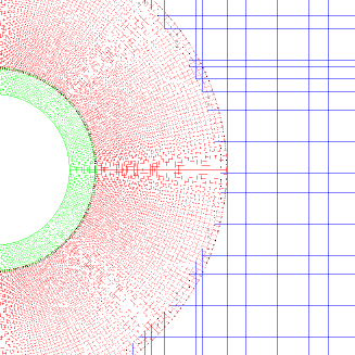
Figure 2: Left: Cropped view of GR4, showing the boundary layer grid (green), transition grid (red) and background grid (blue) with interpolation points. Right: Geometry of the convergence study problem.

In the present work, emphasis is placed on the grid characteristic length scales to optimise run time. Following Nicolle and Eames [54] we use two grid length scales to quantify the quality of the computational grid: the domain length scale (DLS) is the background grid element size while the surface length scale (SLS) is the grid element size on the surface of the particle.

The grid independence study is first performed using a grid with nearly uniform grid spacings and is then repeated using grid refinement near the particle boundary. Descriptions of the grids used are provided in table 1. Because curvilinear grids are used to represent the particles, the cells are slightly distorted in physical space. Thus, table 1 provides minimum, average and maximum cell volumes (areas).

Grid	Node count	Cell volume			DLS	SLS
		min	ave	max
GU1	1497931	0.66	0.678	0.678	$D/96$	$D/96$
GU2	670984	1.47	1.53	1.53	$D/64$	$D/64$
GU3	380394	2.58	2.71	2.71	$D/48$	$D/48$
GU4	171724	5.65	6.10	6.10	$D/32$	$D/32$
GU5	98102	9.90	10.8	10.9	$D/24$	$D/24$
GU6	44967	21.3	24.4	24.4	$D/16$	$D/16$
GR1	679685	0.67	1.52	1.53	$D/64$	$D/96$
GR2	390285	0.78	2.68	2.71	$D/48$	$D/96$
GR3	191265	0.78	5.68	6.10	$D/32$	$D/96$
GR4	123095	0.71	9.09	10.9	$D/24$	$D/96$
GR5	63935	0.78	18.2	24.4	$D/16$	$D/96$
GR6	31455	0.78	39.5	97.7	$D/8$	$D/96$

Table 1: Description of the uniform and refined grids used in the convergence study.

The test used in both convergence studies is as follows: the domain is a rectangular channel of dimensions $(W^{\ast},H^{\ast})=(4\,D,40\,D)$ filled with an a priori quiescent fluid of density $\rho_{f}=1\,\mathrm{g/cm^{3}}$ and kinematic viscosity of $0.05\,\mathrm{cm^{2}/s}$. The particle $(D,\rho_{p})=(0.25,1.5)$ is released from rest at $(x_{0}^{\ast},y_{0}^{\ast})=(D,38.4\,D)$ with the gravitational constant set to $\boldsymbol{g}=981\,\mathrm{cm/s^{2}}$ in the negative $y$-direction. The problem geometry can be seen in Fig. 2. The results are non-dimensionalised as follows:

$$u^{\ast}=\frac{u}{U_{T}},\quad v^{\ast}=\frac{v}{U_{T}},\quad x^{\ast}=\frac{x}{D},\quad y^{\ast}=\frac{y}{D},\quad\omega^{\ast}=\frac{\omega D}{U_{T}},\quad t^{\ast}=\frac{tU_{T}}{D}$$ (9)

where $U_{T}=8.6041\,\mathrm{cm}\,\mathrm{s}^{-1}$ is the measured terminal settling velocity.

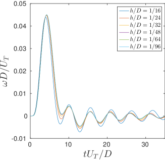
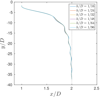
Figure 3: Left: Normalised angular velocity history for the convergence study at increasing grid resolutions. Right: Position of the disk in the channel for the convergence study at increasing grid resolutions.

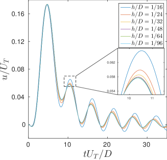
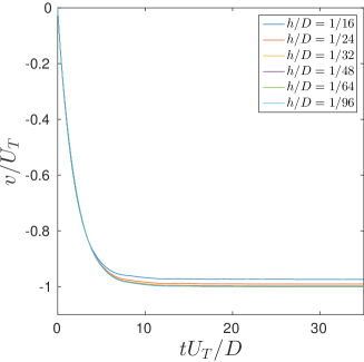
Figure 4: Left: Normalised horizontal velocity history for the convergence study at increasing grid resolutions. Right: Normalised vertical velocity history for the convergence study at increasing grid resolutions.

Under the action of gravity the particle rotates in a clockwise sense, as if rolling down the wall. Immediately after release it moves a short distance towards the near wall before migrating towards its equilibrium position along the channel centreline.

The wake remains attached but is unsteady. This is reflected in the oscillatory $u^{\ast}$ and $\omega^{\ast}$ velocity time histories, shown in figures 4 and 3. The angular velocity time history exhibits a large initial peak after which it is rapidly damped to low amplitude oscillations about $\omega^{\ast}=0$. After a very small negative peak, the $u^{\ast}$ time history exhibits a large positive peak, much like $\omega^{\ast}$, with damped successive peaks. However, unlike in $\omega^{\ast}$, the following $u^{\ast}$ oscillations have a non-zero mean value as the disk drifts towards its equilibrium position. In contrast, the vertical velocity, $v^{\ast}$, shows the particle rapidly reaching a steady settling velocity, unaffected by the attached unsteady wake.

Fig. 5 show relative errors (meaning differences compared to the reference solution) in $v^{\ast}$ and $\omega^{\ast}$, which were calculated as $\epsilon_{v}=(v^{\ast}-v^{\ast}_{\text{ref}})/v^{\ast}_{\text{ref}}$ and $\epsilon_{\omega}=(\omega-\omega^{\ast}_{\text{ref}})/\omega^{\ast}_{\text{ref}}$, where data from the GU1 simulation are used as reference values. Relative errors in $v^{\ast}$ and $\omega^{\ast}$ taken early on in the simulation, at $t=0.2\,\mathrm{s}$, and late in the simulation, at $t=1.0\,\mathrm{s}$, show greater than second order convergence for both components early on but a decrease in convergence rate for $\omega^{\ast}$ as the simulation progresses. The gravitational acceleration is impulsively turned on at $t=0$, and this non-smooth forcing could have a detrimental effect on the convergence rates.

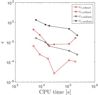
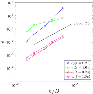
Figure 5: Left: Comparison of relative error magnitude in $v^{\ast}$ and $\omega^{\ast}$ at $t=1\,\mathrm{s}$ against required CPU time using uniform and refinement grids. Right: relative vertical and angular velocity errors at early ($t=0.2\,\mathrm{s}$) and late ($t=1.0\,\mathrm{s}$) stages of the simulation.

The test was repeated using a series of refined grids. These were constructed using a fine grid immediately surrounding the particle surface, smoothly connected to a coarse background grid using a transition grid. This construction can be seen in Fig. 2. Detailed descriptions of the grids are provided in table 1, where uniform grids are denoted by the prefix GU and refinement grids by GR.

Grid	$v/U_{T}$	$u/U_{T}$	$\omega D/U_{T}\times 10^{-4}$	$\epsilon_{v}\times 10^{-4}$	$\epsilon_{u}$	$\epsilon_{\omega}$
GU1	1.0000	0.0033	6.4761	—	—	—
GU2	0.9994	0.0034	6.1663	5.9299	0.0288	0.0521
GU3	0.9994	0.0034	6.8561	14.000	0.0969	0.2275
GU4	0.9957	0.0041	9.2127	43.000	0.2775	0.4609
GU5	0.9900	0.0046	9.4015	100.00	0.4513	0.6093
GU6	0.9734	0.0052	0.0016	266.00	0.6329	1.7913
GR1	0.9995	0.0034	6.5961	1.1599	0.0292	0.0277
GR2	0.9998	0.0033	6.4250	1.6028	0.0141	0.0069
GR3	1.0000	0.0031	6.4250	0.0755	0.0186	0.0062
GR4	1.0002	0.0031	5.8773	2.3025	0.0161	0.0061
GR5	1.0006	0.0032	6.1766	6.0949	0.0013	0.0573
GR6	1.0043	0.0026	6.9848	43.000	0.1915	0.1956

Table 2: Absolute values and relative errors for the convergence study taken at $t=1.0\,\text{s}$.

Table 2 shows absolute values of $u^{\ast}$, $v^{\ast}$ and $\omega^{\ast}$ at $t=1.0\,\mathrm{s}$ as well as relative errors, where data from GU1 were taken as reference values. As before, it is evident that $v^{\ast}$ is fairly insensitive to the grid resolution, while $u^{\ast}$ and $\omega^{\ast}$ show a large dependence on the near surface resolution. With a high resolution surface grid capturing the boundary layer, the motion of the disk can be captured quite accurately, even with a large surface to background grid resolution ratio. In fact, the GR5 grid with a resolution ratio of $6:1$ reproduced solutions of GU1 with a maximum error of $5\,\%$, with a more than 23 fold reduction in number of grid points. Fig. 5 shows the relative error in $v^{\ast}$ and $\omega^{\ast}$ at $t=1\,\mathrm{s}$ against the total CPU time of the calculation.

7.2 Settling disk impacting a wall

This test simulates the fall of a rigid circular disk in a bounded domain and its impact with the bottom boundary. This test has been performed by other researchers using DLM/FDM [26], an FEM fictitious boundary method [72], and an immersed boundary lattice Boltzmann method [36]. The computational domain has a width of $W=8\,D$, a height of $H=24\,D$ and grid characteristic length scales $\textit{DLS}=D/16$ and $\textit{SLS}=D/96$, where $D=0.25\,\mathrm{cm}$ is the disk diameter. The disk is initially placed along the centreline of the domain, $8\,D$ from the top boundary. The disk has density $\rho_{d}=1.25\,\mathrm{g/cm^{3}}$ and the kinematic viscosity of the fluid is $\nu=0.1\,\mathrm{cm^{2}/s}$. The results are non-dimensionalised as in (9), where the characteristic velocity scale $U_{s}$ is an estimated terminal velocity,

$$U_{s}=\sqrt{\frac{\pi D}{2}\left(\frac{\rho_{d}-\rho_{f}}{\rho_{f}}\right)g}.$$ (10)

The present results (Fig. 6) are in good agreement with the previous studies. The disk reaches the terminal settling velocity at $t^{\ast}=20$, with a terminal particle Reynolds number of $\operatorname{Re_{T}=17.45}$, consistent with the literature. As the disk approaches the bottom wall the results differ slightly. The studies compared against in Fig. 6 all exhibit a rebound of the disk from the bottom boundary while the present results do not.

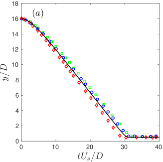
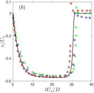
Figure 6: Histories of the $y^{\ast}$-coordinate and $v^{\ast}$ component of the centre of the disk for a low Reynolds number sedimentation of a symmetrically placed disk test case with data from Hu et al.[36] ($\color[rgb]{0,1,0}{\square}$), Wang et al.[72] ($\color[rgb]{0,0,1}{\circ}$), Glowinski et al.[26] ($\color[rgb]{1,0,0}{\lozenge}$) and the present study ($-$).

In the present study the grid around the disk and along the bottom of the tank is very fine ($\textit{SLS}=D/96$ for both the disk and the bottom of the tank), allowing the lubrication forces and flow in the gap to be better resolved. This slows the particle down more before “contact” is made with the wall. Additionally, the present study used a conservation of linear momentum based hard-sphere collision model approach to model the collision between the disk and the bottom boundary. The previous studies compared against here all used repulsive potential type methods. We can estimate a Stokes number for the particle to comment on the “correctness” of the present results. The Stokes number, $\operatorname{Stk}$, is the ratio between the particle and fluid relaxation times, $\tau_{p}$ and $\tau_{f}$, respectively. Taking $\tau_{f}=R/U_{T}$, where $R$ is the disk radius, $\tau_{p}=mv/F_{d}$, and $F_{d}$ is the drag force on the disk, then $\operatorname{Stk}=mv^{2}/(RF_{d})$. Once the disk reaches its terminal settling velocity the drag force balances with the force due to gravity, so $F_{d}=\pi R^{2}g(\rho_{d}-\rho_{f})$ and thus the Stokes number is $\operatorname{Stk}={v^{2}}/(Rg(1-\frac{\rho_{f}}{\rho_{d}}))$. Here, the Stokes number is approximately 2. It has been demonstrated that for 3D cases particles settling with $\operatorname{Stk}<10$ there is no rebound after contact is made with the bottom boundary [2, 39]. Assuming this holds true for the 2D equivalent, then the above results indicate that the repulsive potential collision model is a poor sub-grid model for low speed impacts. The rebound evident in the study of Glowinski et al. [26] indicates that a higher grid resolution is required to adequately resolve the lubrication forces than the hydrodynamic interactions during free-fall. While the current approach is adequate here it is clear that in many situations resolving the gap is not practical and prohibitively expensive. Qiu et al. [61] presented a novel solution to computing incompressible flow in thin gaps using pressure degrees of freedom on virtual solid surfaces to provide solid–fluid coupling in the gap region, which when extended to no-slip boundaries could be a good alternative for this sort of problem.

7.3 Settling of two offset disks

Two offset cylinders settling in a quiescent fluid are simulated to demonstrate the drafting, kissing, tumbling behaviour observed experimentally by Fortes et al. [25]. This is a difficult problem to simulate owing to the non-linear nature of the particle motion and the particle–particle and particle–wall interactions. Results are compared to previous studies of Patankar et al. [57, 56], Wan and Turek [72], Niu et al. [55], Zhang and Prosperetti [76] and Feng and Michaelides [23] for a low Reynolds number case and Uhlmann [67] for a moderate Reynolds number case. The low Reynolds number case uses a computational domain of width $10\,D$ and height $40\,D$, with the particles of diameter $0.2\,\mathrm{cm}$ placed along the vertical centreline, $4\,D$ and $6\,D$ from the top boundary. The high Reynolds number case uses a computational domain of width $8\,D$ and height $24\,D$, with the particles of diameter $0.25\,\mathrm{cm}$ placed $4\,D$ and $6\,D$ from the top boundary, and offset by $D/250$ and $-D/250$ from the vertical centreline. For the low Reynolds number case, the grid characteristic length scales are $\textit{DLS}=D/19$ and $\textit{SLS}=D/76$ whilst for the moderate Reynolds number case $\textit{DLS}=D/24$ and $\textit{SLS}=D/128$. In each case, both the top and bottom particles have the same density ratio. For the low Reynolds number case, the density ratio is $\rho_{r}=1.01$ and the fluid has kinematic viscosity $\nu=0.1\,\mathrm{cm^{2}/s}$. For the moderate Reynolds number case, the density ratio is $\rho_{r}=1.5$ and the kinematic viscosity is $\nu=0.01\,\mathrm{cm^{2}/s}$. In both cases the gravitational constant was taken as $\boldsymbol{g}=981\,\mathrm{cm}/\mathrm{s}^{2}$ and the results are non-dimensionalised as in (9), where the characteristic velocity, $U_{s}$, is again calculated using (10).

Figure 7: Settling of two disks in a quiescent fluid. Contours of the vorticity at five different time, with a vorticity scale between $-3.6\leq\xi D/U_{s}\leq 3.6$.

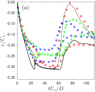
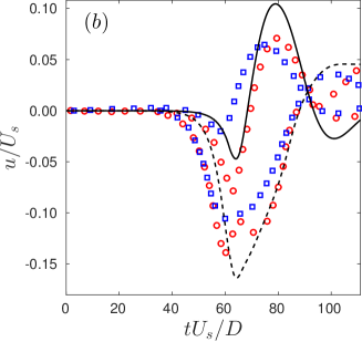
Figure 8: Histories of the $(a)$ $v^{\ast}$ and $(b)$ $u^{\ast}$ velocity components of the centre of the disks for the low Reynolds number drafting, kissing, and tumbling test case, with $\rho_{d}=1.01$, $\nu=0.1$ where the solid line denotes the (initially) top disk and the dashed line the bottom disk, with data from: $(a)$ Patankar [56] ($\color[rgb]{0,1,0}{\lozenge}$), Patankar et al. [57] ($\color[rgb]{0,0,1}{\square}$) and Feng et al. [23] ($\color[rgb]{1,0,0}\circ$); $(b)$ Patankar et al. [57] ($\color[rgb]{0,0,1}{\square}$) and Feng et al. [23] ($\color[rgb]{1,0,0}\circ$) overlayed.

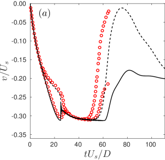
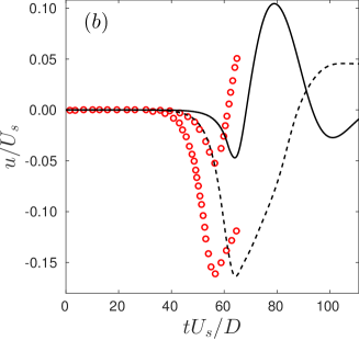
Figure 9: Time histories of the $(a)$ $v^{\ast}$ and $(b)$ $u^{\ast}$ velocity components of the centre of the disks for the low Reynolds number drafting, kissing, and tumbling test case with $\rho_{d}=1.01$, $\nu=0.1$, where the solid line denotes the (initially) top disk and the dashed line the bottom disk, and data from Zhang et al. [76] overlayed ($\color[rgb]{1,0,0}\circ$).

Fig. 7 shows the positions of the particles as they sediment, interacting with each other and the domain boundary, along with instantaneous vorticity contours. The observed dynamical interactions are in good agreement with those observed in the quasi two-dimensional experiments in [25]. Initially, the two particles begin moving from rest under the influence of gravity with the same acceleration. As the wake forms behind the lower particle the top particle becomes shielded in the resultant low pressure region. This allows the top particle to draft behind the lower particle, similar to cyclists in a peloton. This is the “drafting” stage. Eventually, the top particle makes near contact with the lower particle (they “kiss”) and effectively form an elongated body with axis parallel to the fall. This configuration is inherently unstable and the elongated body rotates to align its long axis perpendicular to the fall. This is the “tumbling” stage described in [25]. The particles separate and the lower particle is overtaken by the top particle, which continues to sediment with a slightly negative $u^{\ast}$ velocity. The other particle impacts the wall, after which it, too, sediments with a slightly negative $u^{\ast}$ velocity.

The results for the low Reynolds number case compare well qualitatively with those of [57, 56, 23] but not quantitatively (see Fig. 8). Though quantitative agreement is not necessarily apparent amongst the results of these studies themselves, what is apparent is that their settling velocities are all lower than those found in the present study. Although different methods were used, all three of these simulations used low grid resolutions around the particles, particularly [23]. The study in [76] used a higher resolution grid, with 20 computational nodes per particle diameter. Very good quantitative agreement is found between that study and the present one, as is evident from figure 9, though there is a discrepancy in the duration of the “kissing” contact and the onset of “tumbling”. The onset of “tumbling” is caused by the build up of numerical error, so this is expected to be solver specific. In the absence of numerical error, or bias introduced by the grid, the disks would not leave the “kissing” stage [67].

Figure 10: Time histories of $x^{\ast}$, $y^{\ast}$, $v^{\ast}$, $u^{\ast}$ and $\omega^{*}$ for the moderate Reynolds number drafting, kissing, and tumbling test case with $\rho_{d}=1.5$, $\nu=0.01$, where the solid line denotes the (initially) top disk and the dashed line the bottom, and data from Uhlmann [67] overlayed ($\color[rgb]{1,0,0}\circ$).

Results for the moderate Reynolds number case are shown in Fig. 10. These are compared to results from [67], who used an immersed boundary method on high resolution grids. Both qualitatively and quantitatively the results are in excellent agreement for the particle positions and $u,v$ velocity components, with the only differences found during the initial contact and subsequent “kissing” stage, due to the different collision models. All of the aforementioned studies used a repulsive force based model, while a conservation of linear momentum model is used here. Fig. 10 shows good qualitative but poor quantitative agreement for the angular velocity component. This is a very sensitive metric [67] and it is likely that the differences are due, in large part, to the different collision mechanisms used. The novel approach of Kempe and Fröhlich [42], which uses a sub-grid lubrication force correction and conserves angular momentum, would probably be a more appropriate collision mechanism for this case.

7.4 Two particle wake interaction

Figure 11: Problem geometry for the two particle wake interaction test case.

This is a case presented by Uhlmann [67] to test the fluid–structure interaction, with particular emphasis on examining the effect of wake interactions between the particles on the angular velocity. Two particles of differing densities settle in an otherwise quiescent fluid. The heavier particle passes the lighter particle, subjecting it to perturbations from its wake. The particles do not collide and therefore no collision model is required, making it an attractive benchmark case.

Figure 12: Contours of vorticity at times $t=0.8$, $t=3.2$, $t=5.6$, $t=8.0$ for the pure wake interaction test case compared to plots from Uhlmann [67] taken at the same times and with the same vorticity extrema. Left: present study using a quasi uniform grid with DLS=D/40 and SLS=D/40. Right: results from [67] computed on a uniform grid of resolution $D/40$.

The computational domain, shown in Fig. 11, has a width of $10\,D$, a height of $50\,D$ and the grid characteristic length scales are $\textit{DLS}=D/40$ and $\textit{SLS}=D/100$, where the particle diameter is $D=0.2\,\mathrm{m}$. A heavier particle of density ratio $\rho_{r,1}=1.5$ is initially positioned at $\boldsymbol{x}=(-0.65\,D,4\,D)$ from the channel centreline and top boundary respectively, while the lighter particle of density ratio $\rho_{r,2}=1.25$ is positioned at $\boldsymbol{x}=(0.65\,D,6\,D)$. Both particles are initially at rest and the fluid of kinematic viscosity $\nu=0.0008\,\mathrm{m^{2}/s}$ is quiescent at $t=0\,\mathrm{s}$. The gravitational constant is set to $\boldsymbol{g}=9.81\,\mathrm{m/s^{2}}$. The results are non-dimensionalised as in (9), where the characteristic velocity $U_{s}$ is calculated using (10) and the density ratio of the heavier disk, viz. $\rho_{r,1}=1.5$.

Figure 13: Time histories of $x^{\ast}$, $y^{\ast}$, $v^{\ast}$, $u^{\ast}$ and $\omega^{*}$ for the pure wake interaction test case with $\rho_{r,1}=1.5$, $\rho_{r,2}=1.25$, $\nu=0.0008\,\mathrm{m^{2}/s}$ and data from Uhlman [67] overlayed.

The maximum particle Reynolds numbers of the heavy and light particle are 280 and 230, respectively [67]. Uhlmann [67] used a uniform grid resolution of $\textit{DLS}=D/40$, allowing for fewer than three grid points across the estimated boundary layer depth for both the light and heavy particles. Given the findings of the convergence study in section 7.1 it is not likely that the solutions at this grid resolution are grid independent. A brief convergence study was performed, shown in table 3, and solutions were found to converge at $\textit{SLS}=D/100$, allowing for 6 points across the boundary layers for both the light and heavy particle.

SLS	$u/U_{s}$	$v/U_{s}$	$\omega D/U_{s}$	$\epsilon_{u}$	$\epsilon_{v}$	$\epsilon_{\omega}$
D/200	0.14550	-0.36470	-0.01123	—	—	—
D/150	0.14554	-0.36483	-0.01225	0.00028	0.00033	0.00181
D/100	0.14567	-0.36518	-0.01132	0.00121	0.00130	0.00831
D/50	0.14680	-0.36705	-0.01205	0.00896	0.00643	0.07353
D/40	0.01479	-0.36847	-0.01293	0.01644	0.01033	0.15205

Table 3: Absolute values and relative errors for disk 2 taken at $t=1\,\mathrm{s}$ of the wake interaction grid independence study.

Fig. 12 shows successive snapshots of the instantaneous vorticity field with snapshots from [67] below. The evolving flow field and particle positions match well. Fig. 13 shows the time histories of the particles position, velocity and angular velocity.

The converged solutions of the present study match well with those in [67], although a phase shift is apparent in the oscillatory components and the settling velocity is slightly higher in the present study.

The largest differences are found in the horizontal velocity components, particularly for the light particle. These differences are probably due in large part to the differences in the angular velocity components, which will affect vortex shedding and lift on the particles. The amplitudes of the angular velocity component oscillations for the heavier particle match well but a slight phase shift is apparent. This is reflected in the horizontal velocity components for the heavier particle by matching amplitudes but markedly different periods of oscillation. The angular velocity components of the lighter particle differ in both amplitude and period of oscillation, leading to more pronounced differences in the horizontal velocity components of the two studies.

7.5 Settling sphere

As a final validation case we compare experimental [65] and numerical [74] results on the motion of a single sphere in a closely confined container to numerical results produced by the current method. Four cases were run, with Reynolds numbers ranging from 1.5 to a moderate 31.9. The material parameters used in each case are detailed in table 4, with $\boldsymbol{g}=9.81\,\mathrm{m/s^{2}}$ throughout. For each case the grid characteristic length scales are $\textit{DLS}=D/10$ and $\textit{SLS}=D/38$, allowing for approximately six points across the estimated boundary layer depth for the highest Reynolds number case.

Case number	$\rho_{f}$	$\mu_{f}$	$\operatorname{Re}$	$\operatorname{Stk}$
	[$\mathrm{kg}/\mathrm{m}^{3}$]	[$\mathrm{N}\,\mathrm{s}/\mathrm{m}^{2}$]	[–]	[–]
1	970	0.373	1.5	0.19
2	965	0.212	4.1	0.53
3	962	0.113	11.6	1.50
4	960	0.058	31.9	4.13

Table 4: Parameters used for the four settling sphere cases.

The sphere undergoes three distinct periods of motion after its release from rest: an initial acceleration followed by a period of steady fall at a terminal settling velocity and finally a deceleration as it approaches the wall. As the Reynolds number is increased the three stages become progressively shorter. Similar to Yang and Stern [74] the wall collisions were not considered here and the simulations stopped before the sphere made contact with the wall.

The present results are shown in Fig. 14 and match satisfactorily with the experimental results of ten Cate et al. [65] although some slight differences remain: the terminal settling velocity in case 1 is found to be approximately $4.6\,\%$ lower here and in case 2 the sphere begins the wall induced deceleration sooner than in [65]. This earlier deceleration in case 2 is also present in the results of [74], as is the lower terminal settling velocity of case 1. The benefit of using overset grids is again evident; the grid used above consists of $5.18\times 10^{5}$ grid points while the results are as good as those produced on a uniform grid over three times the size.

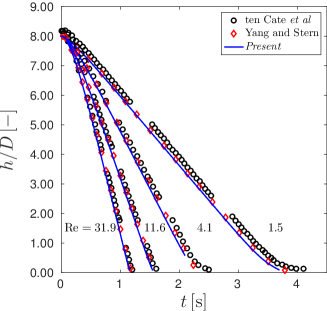
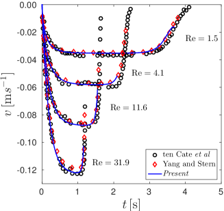
Figure 14: Left: non-dimensionalised vertical position of the sphere compared to numerical results of Yang et al. [74] ($\color[rgb]{1,0,0}{\lozenge}$) and experimental results of ten Cate et al. [65] ($\circ$). Right: dimensional vertical velocity of the sphere compared to numerical results of [74] ($\color[rgb]{1,0,0}{\lozenge}$) and experimental results of [65] ($\circ$).

8 Conclusion

We evaluated the overset grid method for DNS of viscous, incompressible fluid flow with rigid, moving bodies. Several FSI benchmark test cases were carried out for verification and validation purposes. A systematic convergence test was carried out using six uniformly refined grids and six with local refinement near the particle surface. Local refinement was found to produce results deviating no more than five percent from the reference solutions, with a more than 23 fold decrease in grid point count and a subsequent 13 fold decrease in CPU time.

Finally, results for a sphere settling in a small tank at various Reynolds numbers compared well with both experimental results of ten Cate et al. [65] and recent numerical results of Yang et al. [74], using only one third the number of grid points as the latter study.

The popular test cases presented in this work are all, to varying degrees, inertially dominated and exhibit viscous boundary layers that must be fully resolved to accurately simulate the behaviour of the rigid bodies in the flow. The second-order accurate boundary fitted method demonstrated here was found to produce reasonably converged results with approximately six grid points across the estimated boundary layer depth. By using a coarse—but fine enough to resolve wake structures—Cartesian background grid and refined, boundary-fitted grids, grid point counts were greatly reduced, even in two-dimensional problems.

The overset grid method has shown promising capabilities for fully-resolved DNS of small numbers of rigid particles. With a more sophisticated collision mechanism, e.g. the multi-scale approach of Kempe et al. [40] or the DEM approach of Wachs [70], fully-resolved DNS of larger numbers of arbitrarily shaped particles could be performed. Without modification to the underlying discretisation technique other types of flow, for example arbitrarily moving bodies in non-Newtonian flows, could be examined.

References

References

- Almgren et al. [1998] Almgren, A. S., Bell, J. B., Colella, P., Howell, L. H., Welcome, M. L., 1998. A conservative adaptive projection method for the variable density incompressible Navier–Stokes equations. J. Comput. Phys. 142, 1–46.
- Ardekani and Rangel [2008] Ardekani, A. M., Rangel, R. H., 2008. Numerical investigation of particle–particle and particle–wall collisions in a viscous fluid. J. Fluid Mech. 596, 437–466.
- Bagchi [2007] Bagchi, P., 2007. Mesoscale simulation of blood flow in small vessels. Biophys. J. 92, 1858–1877.
- Balay et al. [2013] Balay, S., Brown, J., Buschelman, K., Eijkhout, V., Gropp, W. D., Kaushik, D., Knepley, M. G., McInnes, L. C., Smith, B. F., Zhang, H., 2013. PETSc users manual. Tech. rep., Argonne National Laboratory.
- Banks et al. [2016] Banks, J. W., Henshaw, W. D., Kapila, A., Schwendeman, D. W., 2016. An added-mass partitioned algorithm for fluid-structure interactions of compressible fluids and nonlinear solids. J. Comput. Phys. 305, 1037–1064.
- Banks et al. [2012] Banks, J. W., Henshaw, W. D., Schwendeman, D. W., 2012. Deforming composite grids for solving fluid structure problems. J. Comput. Phys. 231 (9), 3518–3547.
- Banks et al. [2014a] Banks, J. W., Henshaw, W. D., Schwendeman, D. W., 2014a. An analysis of a new stable partitioned algorithm for FSI problems. Part I: incompressible flow and elastic solids. J. Comput. Phys. 269, 108–137.
- Banks et al. [2014b] Banks, J. W., Henshaw, W. D., Schwendeman, D. W., 2014b. An analysis of a new stable partitioned algorithm for FSI problems. Part II: Incompressible flow and structural shells. J. Comput. Phys. 268, 399–416.
- Banks et al. [2013] Banks, J. W., Henshaw, W. D., Sjögreen, B., 2013. A stable FSI algorithm for light rigid bodies in compressible flow. J. Comput. Phys. 245, 399–430.
- Batchelor [1967] Batchelor, G. K., 1967. An introduction to fluid dynamics. Cambridge University Press.
- Behr and Tezduyar [1994] Behr, M., Tezduyar, T. E., 1994. Finite element strategies for large-scale flow simulations. Comput. Methods Appl. Mech. Engrg. 112, 3–24.
- Borazjani et al. [2008] Borazjani, I., Ge, L., Sotiropoulos, F., 2008. Curvilinear immersed boundary method for simulating fluid structure interaction with complex 3D rigid bodies. J. Comput. Phys. 227 (16), 7587–7620.
- Brady [1988] Brady, J. F., 1988. Stokesian dynamics. Annu. Rev. Fluid Mech. 20, 111–157.
- Broering et al. [2012] Broering, T., Lian, Y., Henshaw, W., 2012. Numerical investigation of energy extraction in a tandem flapping wing configuration. AIAA Journal 50 (11), 2295–2307.
- Chan [2009] Chan, W. M., 2009. Overset grid technology development at NASA Ames Research Center. Comput. Fl. 38 (3), 496–503.
- Chandar and Damodaran [2010] Chandar, D. D. J., Damodaran, M., 2010. Numerical study of the free flight characteristics of a flapping wing in low Reynolds numbers. AIAA J. Aircraft 47 (1), 141–150.
- Chesshire and Henshaw [1990] Chesshire, G. S., Henshaw, W. D., 1990. Composite overlapping meshes for the solution of partial differential equations. J. Comput. Phys. 90 (1), 1–64.
- Chesshire and Henshaw [1994] Chesshire, G. S., Henshaw, W. D., July 1994. A scheme for conservative interpolation on overlapping grids. SIAM J. Sci. Comput. 15 (4), 819–845.
- Dougherty and Kuan [1989] Dougherty, F. C., Kuan, J.-H., 1989. Transonic store separation using a three-dimensional Chimera grid scheme. paper 89-0637, AIAA.
- English et al. [2013] English, R. E., Qiu, L., Yu, Y., Fedkiw, R., 2013. An adaptive discretization of incompressible flow using a multitude of moving Cartesian grids. J. Comput. Phys. 254, 107–154.
- Fadlun et al. [2000] Fadlun, E. A., Verzicco, R., Orlandi, P., Mohd-Yusof, J., 2000. Combined immersed-boundary finite-difference methods for three-dimensional complex flow simulations. J. Comput. Phys. 161, 35–60.
- Falgout and Yang [2002] Falgout, R. D., Yang, U. M., 2002. hypre: a library of high performance preconditioners. Springer Berlin Heidelberg.
- Feng and Michaelides [2004] Feng, Z.-G., Michaelides, E. E., 2004. The immersed boundary-lattice Boltzmann method for solving fluid–particles interaction problems. J. Comput. Phys. 195, 602–628.
- Ferziger and Perić [2002] Ferziger, J. H., Perić, M., 2002. Computational methods for fluid dynamics, 3rd Edition. Springer.
- Fortes et al. [1987] Fortes, A. F., Joseph, D. D., Lundgren, T. S., 1987. Nonlinear mechanics of fluidization of beds of spherical particles. J. Fluid Mech. 177, 467–483.
- Glowinski et al. [2001] Glowinski, R., Pan, T. W., Hesla, T. I., Joseph, D. D., Périaux, J., 2001. A fictitious domain approach to the direct numerical simulation of incompressible viscous flow past moving rigid bodies: Application to particulate flow. J. Comput. Phys. 169, 363–426.
- Haeri and Shrimpton [2012] Haeri, S., Shrimpton, J. S., 2012. On the application of immersed boundary, ficticious domain and body-conformal mesh methods to many particle multiphase flows. Int. J. Multiphas. Flow 40, 38–55.
- Henshaw [1994] Henshaw, W. D., 1994. A fourth-order accurate method for the incompressible Navier–Stokes equations on overlapping grids. J. Comput. Phys. 113, 13–25.
- Henshaw [1998] Henshaw, W. D., 1998. Ogen: An overlapping grid generator for Overture. Research Report UCRL-MA-132237, Lawrence Livermore National Laboratory.
- Henshaw [2005] Henshaw, W. D., 2005. On multigrid for overlapping grids. SIAM J. Sci. Comput. 26 (5), 1547–1572.
- Henshaw and Petersson [2001] Henshaw, W. D., Petersson, N. A., 2001. A split-step scheme for the incompressible Navier–Stokes equations. Tech. rep., Centre for Applied Scientific Computing, Lawrence Livermore National Laboratory, Livermore, CA, 94551.
- Henshaw and Petersson [2003] Henshaw, W. D., Petersson, N. A., 2003. A split-step scheme for the incompressible Navier-Stokes equations. In: Hafez, M. M. (Ed.), Numerical Simulation of Incompressible Flows. World Scientific, pp. 108–125.
- Henshaw and Schwendeman [2006] Henshaw, W. D., Schwendeman, D. W., 2006. Moving overlapping grids with adaptive mesh refinement for high-speed reactive and non-reactive flow. J. Comput. Phys. 216 (2), 744–779.
- Hu [1996] Hu, H. H., 1996. Direct simulation of flows of solid–liquid mixtures. Int. J. Multiphas. Flow 22 (2), 335–352.
- Hu et al. [2001] Hu, H. H., Patankar, N. A., Zhu, M. Y., 2001. Direct numerical simulations of fluid–solid systems using the arbitrary Lagrangian–Eulerian technique. J. Comput. Phys. 169, 427–462.
- Hu et al. [2015] Hu, Y., Li, D., Shu, S., Niu, X., 2015. Modified momentum exchange method for fluid–particle interactions in the lattice Boltzmann method. Phys. Rev. E 91.
- Hughes et al. [1981] Hughes, T. J. R., Liu, W. K., Zimmermann, T. K., 1981. Lagrangian–Eulerian finite element formulation for incompressible viscous flows. Comput. Methods Appl. Mech. Engrg. 29, 329–349.
- Johnson and Tezduyar [1996] Johnson, A. A., Tezduyar, T. E., 1996. Simulation of multiple spheres falling in a liquid-filled tube. Comput. Methods Appl. Mech. Engrg. 134, 351–373.
- Joseph et al. [2001] Joseph, G. G., Zenit, R., Hunt, M. L., Rosenwinkel, A. M., 2001. Particle–wall collisions in a viscous fluid. J. Fluid Mech. 433, 329–346.
- Kempe and Fröhlich [2012a] Kempe, T., Fröhlich, J., 2012a. Colision modelling for the interface-resolved simulation of spherical particles in viscous fluids. J. Fluid Mech. 709, 445–489.
- Kempe and Fröhlich [2012b] Kempe, T., Fröhlich, J., 2012b. An improved immersed boundary method with direct forcing for the simulation of particle laden flows. J. Comput. Phys. 231, 3663–3684.
- Kempe and Fröhlich [2012] Kempe, T., Fröhlich, J., 2012. An improved immersed boundary method with direct forcing for the simulation of particle laden flows. J. Comput. Phys. 231 (9), 3663–3684.
- Kim and Choi [2006] Kim, D., Choi, H., 2006. Immersed boundary method for flow around an arbitrarily moving body. J. Comput. Phys. 212, 662–680.
- Kushch et al. [2002] Kushch, V. I., Sangani, A. S., Spelt, P. D. M., Koch, D. L., 2002. Finite-Weber-number motion of bubbles through a nearly inviscid liquid. J. Fluid Mech. 460, 241–280.
- Küttler and Wall [2008] Küttler, U., Wall, W. A., 2008. Fixed-point fluid–structure interaction solvers with dynamic relaxation. Computational Mechanics 43 (1), 61–72.
- Lani et al. [2012] Lani, A., Sjögreen, B., Yee, H. C., Henshaw, W. D., 2012. Variable high-order multiblock overlapping grid methods for mixed steady and unsteady multiscale viscous flows, part II: hypersonic nonequilibrium flows. Commun. Comput. Phys. 13 (2), 583–602.
- Li et al. [2016] Li, L., Henshaw, W. D., Banks, J. W., Schwendeman, D. W., Main, G. A., 2016. A stable partitioned FSI algorithm for incompressible flow and deforming beams. J. Comput. Phys. 312, 272–306.
- Luo et al. [2012] Luo, H., Dai, H., Ferreira de Sousa, P. J. S. A., Yin, B., 2012. On the numerical oscillation of the direct-forcing immersed-boundary method for moving boundaries. Comput. Fluids 56, 61–76.
- Meakin [1993] Meakin, R., 1993. Moving body overset grid methods for complete aircraft tiltrotor simulations. paper 93-3350, AIAA.
- Mittal and Iccarino [2005] Mittal, R., Iccarino, G., 2005. Immersed boundary methods. Annu. Rev. Fluid Mech. 37, 239–261.
- Mohd-Yusof [1997] Mohd-Yusof, J., 1997. Combined immersed-boundary/B-spline methods for simulations of flow in complex geometries. Center for Turbulence Research Annual Research Briefs.
- Nelson and Guillot [2006] Nelson, E. B., Guillot, D., 2006. Well cementing, 2nd Edition. Schlumberger.
- Nicolle [2010] Nicolle, A., 2010. Flow through and around groups of bodies. Ph.D. thesis, University College London.
- Nicolle and Eames [2011] Nicolle, A., Eames, I., 2011. Numerical study of flow through and around a circular array of cylinders. J. Fluid Mech. 679, 1–31.
- Niu et al. [2006] Niu, X. D., Shu, C., Chew, Y. T., Peng, Y., 2006. A momentum exchange-based immersed boundary-lattice Boltzmann method for simulating incompressible viscous flows. Phys. Lett. A 354, 173–182.
- Patankar [2001] Patankar, N. A., 2001. A formulation for fast computations of rigid particulate flows. Center for Turbulence Research.
- Patankar et al. [2000] Patankar, N. A., Singh, P., Joseph, D. D., Glowinski, R., Pan, T.-W., 2000. A new formulation of the distributed Lagrange multiplier/fictitious domain method for particulate flows. Int. J. Multiphas. Flow 26, 1509–1524.
- Patankar and Spalding [1972] Patankar, S. V., Spalding, D. B., 1972. A calculation procedure for heat, mass and momentum transfer in three-dimensional parabolic flows. Int. J. Heat Mass Transfer 15, 1787–1806.
- Peskin [1972] Peskin, C. S., 1972. Flow patterns around heart valves: a numerical method. J. Comput. Phys. 10, 252–271.
- Petersson [2001] Petersson, N. A., 2001. Stability of pressure boundary conditions for Stokes and Navier–Stokes equations. J. Comput. Phys. 172, 40–70.
- Qiu et al. [2015] Qiu, L., Yu, Y., Fedkiw, R., 2015. On thin gaps between rigid bodies two-way coupled to incompressible flow. J. Comput. Phys. 292, 1–29.
- Sangani and Didwania [1993] Sangani, A. S., Didwania, A. K., 1993. Dynamic simulations of flows of bubbly liquids at large Reynolds numbers. J. Fluid Mech. 250, 307–337.
- Seo and Mittal [2011] Seo, J. H., Mittal, R., 2011. A sharp-interface immersed boundary method with improved mass conservation and reduced spurious pressure oscillations. J. Comput. Phys. 230, 7347–7363.
- Tang et al. [2003] Tang, H. S., Jones, S. C., Sotiropoulos, F., 2003. An overset-grid method for 3D unsteady incompressible flows. J. Comput. Phys. 191, 567–600.
- ten Cate et al. [2002] ten Cate, A., Nieuwstad, C. H., Derksen, J. J., Van den Akker, H. E. A., 2002. Particle imaging velocimetry experiments and lattice-Boltzmann simulations on a single sphere settling under gravity. Phys. Fluids 11.
- Tezduyar et al. [1992] Tezduyar, T. E., Behr, M., Liou, J., 1992. A new strategy for finite element computations involving moving boundaries and interfaces – the deforming-spatial-domain/space-time procodure: I. The concept and the preliminary numerical tests. Comput. Methods Appl. Mech. Engrg. 94, 339–351.
- Uhlmann [2005] Uhlmann, M., 2005. An immersed boundary method with direct forcing for the simulation of particulate flows. J. Comput. Phys. 209, 448–476.
- Uhlmann and Doychev [2014] Uhlmann, M., Doychev, T., 2014. Sedimentation of a dilute suspension of rigid spheres at intermediate Galileo numbers: the effect of clustering upon the particle motion. J. Fluid Mech. 752, 310–348.
- Vowinckel et al. [2014] Vowinckel, B., Kempe, T., Fröhlich, J., 2014. Fluid–particle interaction in turbulent open channel flow with fully-resolved mobile beds. Adv. Water Resour. 72, 32–44.
- Wachs [2009] Wachs, A., 2009. A DEM-DLM/FD method for direct numerical simulation of particulate flows: Sedimentation of polygonal isometric particles in a Newtonian fluid with collisions. Comput. Fluids 38, 1608–1628.
- Wachs et al. [2015] Wachs, A., Hammouti, A., Vinay, G., Rahmani, M., 2015. Accuracy of finite volume/staggered grid distributed Lagrange multiplier/fictitious domain simulations of particulate flows. Comput. Fluids 115, 154–172.
- Wan and Turek [2006] Wan, D., Turek, S., 2006. Direct numerical simulation of particulate flow via multigrid FEM techniques and the fictitious boundary method. Int. J. Numer. Meth. Fl. 51, 531–566.
- Yang and Balaras [2006] Yang, J., Balaras, E., 2006. An embedded-boundary formulation for large-eddy simulation of turbulent flows interacting with moving boundaries. J. Comput. Phys. 215, 12–40.
- Yang and Stern [2015] Yang, J., Stern, F., 2015. A non-iterative direct forcing immersed boundary method for strongly-coupled fluid-solid interactions. J. Comput. Phys. 295 (779–804).
- Zahle et al. [2007] Zahle, F., Johansen, J., Sørensen, N. N., Graham, J. M. R., 2007. Wind turbine rotor-tower interaction using an incompressible overset grid method. paper 2007-425, AIAA.
- Zhang and Prosperetti [2003] Zhang, Z., Prosperetti, A., 2003. A method for particle simulation. ASME 70, 64–74.