A Monte Carlo wavefunction description of losses in a 1D Bose gas and cooling to the ground state by quantum feedback

Abstract

The effect of atom losses on a homogeneous one-dimensional Bose gas lying within the quasi-condensate regime is investigated using a Monte Carlo wavefunction approach. The evolution of the system is calculated, conditioned by the loss sequence, namely the times of individual losses and the position of the removed atoms. We describe the gas within the linearized Bogoliubov approach. For each mode, we find that, for a given quantum trajectory, the state of the system converges towards a coherent state, i.e. the ground state, displaced in phase space. Provided losses are recorded with a temporal and spatially resolved detector, we show that quantum feedback can be implemented and cooling to the ground state of one or several modes can be realized.

In Grišins et al. (2016), the effect of atom losses on a one-dimensional quasi-condensate was investigated. The authors have shown that, within a linearized approach and for a large enough initial temperature, one expects the temperature of the low lying modes to decrease in time, in agreement with recent experimental results Rauer et al. (2016). The fluctuations induced by the loss process due to the discrete nature of atoms is however responsible for a heating, limiting the temperature which can be achieved. More precisely, one expects that the temperature asymptotically converges towards $g\rho(t)$ where $g$ is the coupling constant and $\rho$ the linear atomic density Grišins et al. (2016); Note . In particular, excitations in the phononic regime, i.e. of frequency much smaller than $g\rho(t)/\hbar$, never enter the quantum regime: their mean occupation number stays very large such that they lie in the Raighley-Jeans regime. This heating only occurs if one ignores the results of the losses, or, equivalently, if one takes the the partial trace on the state of the reservoir in which losses occur, ending up with the Master equation for the system’s density matrix. If on the other hand, one records the losses, more information is gained on the system and the analysis made in Grišins et al. (2016) is no longer sufficient.

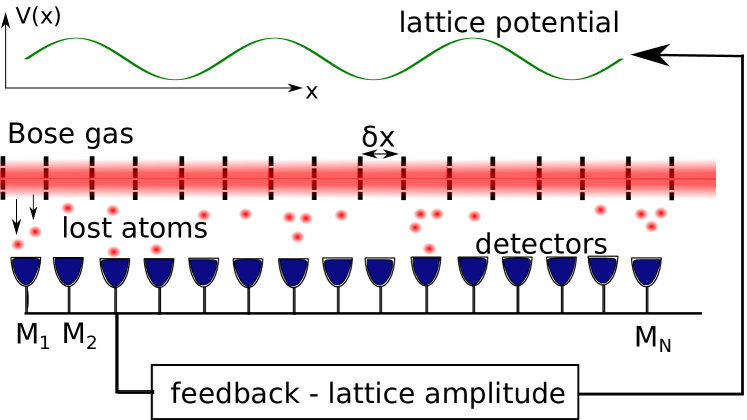
Figure 1: A one-dimensional Bose gas with atom losses and a spatially resolved single atom detectors system. The information on the atom loss can be used to create a feedback loop on the atoms via a lattice potential. The amplitude of the lattice potential is controlled by a processing unit which uses the information gained from the atom losses.

In this paper, we assume the losses are monitored with a spatially and temporally resolved detector and we describe the evolution of the system using a Monte Carlo wavefunction analysis. The measurement back action leads to an evolution of the system conditioned by the result of the loss process, namely a given history of losses. Averaging over the different possible histories, the results of Grišins et al. (2016) are recovered. The analysis proposed in this paper however not only presents an alternative picture conveying more physical insight, but it also opens the road to the realization of measurement based quantum feedback: controlled dynamics, conditioned on the monitored losses, allows to reach lower temperatures. In this paper, we show that feedback on a given mode of the system could in principle allow to cool this mode to the ground state. In particular we show that phononic excitations can be brought to the quantum regime. State preparation using information inferred from losses has already been used to prepare a well defined phase between two condensates Saba et al. (2005), with a Monte Carlo wavefunction approach providing a very clear understanding of the mechanism Castin and Dalibard (1997). Manipulation of cold atomic clouds by quantum feedback has been proposed in many theoretical papers using dispersive light-atom interaction Szigeti et al. (2009); Wade et al. (2015), while feedback has been implemented for internal degrees of freedom Vanderbruggen et al. (2013); Vasilakis et al. (2015); Kuzmich et al. (2000).

Discretization of the problem.

We consider a one-dimensional Bose gas with contact repulsive interactions of coupling constant $g$, such that the Hamiltonian writes, in second quantization,

$$H=-\frac{\hbar^{2}}{2m}\!\int\!dx\psi^{+}\partial^{2}\psi/\partial x^{2}+\frac{g}{2}\!\int\!dx\psi^{+}(x)\psi^{+}(x)\psi(x)\psi(x).$$

We assume the gas is submitted to atom losses, the loss mechanism being a single atom process described by a loss rate $\Gamma$. For instance, magnetically trapped atoms could be submitted to a radio-frequency field that would transfer atoms to an untrapped state, as realized experimentally in Rauer et al. (2016). Atoms could also be ionized by laser fields Kraft et al. (2007), or expelled by collision with fast electrons Gericke et al. (2008). We moreover assume the lost atoms are detected one by one with position-resolved detectors, as sketched in Fig. (1). We note $\bar{\rho}$ the mean linear density and we assume the gas lies within the quasi-condensate regime such that the atomic density fluctuations are small and their characteristic length scale, equal to the healing length $l_{h}=\hbar/\sqrt{mg\bar{\rho}}$, is much larger than the mean interparticle distance Mora and Castin (2003). We discretize space in $N$ cells of length $\delta x$, containing a large mean atom number $\bar{n}=\delta x\bar{\rho}$ and with small relative fluctuations. We furthermore assume that $\delta x$ is large enough such that the fluctuations are large compared to unity. The state of the gas may be expanded (as long as one is not interested in length scales smaller than $\delta x$) on the Fock basis of each cell

$$|\psi\rangle=\sum_{n_{1},n_{2},\dots,n_{N}}c_{n_{1},n_{2},\dots,n_{N}}|n_{1},n_{2},\dots,n_{N}\rangle.$$ (1)

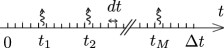
Figure 2: A typical loss sequence during a time interval $\Delta t$, for a single cell. The associated quantum trajectory followed by the system’s wavefunction is given by Eq. 2.

Time is also discretized in intervals $\Delta t$ small compared to the time scales involved in the longitudinal dynamics of the gas. This allows to consider, during $\Delta t$, the sole effect of losses first and then the effect of the free evolution. We will first concentrate on the effect of losses. Since losses do not introduce correlations between different cells, it is relevant to consider the case of a single cell first.

Monte Carlo description of losses in a single cell.

Considering a single cell, the initial state writes $|\psi(t)\rangle=\sum_{n}c_{n}|n\rangle$. Let us split $\Delta t$ in elementary time steps of length $dt$, small enough so that the probability to have an atom lost during $dt$ is small. According to the Monte Carlo wavefunction procedure Mølmer and Castin (1996), if no atoms are detected during a time step $dt$, then the state of the system evolves according to the non Hermitian Hamiltonian $H_{\rm{eff}}=-i\hbar\Gamma a^{+}a/2$, which ensures the decrease of the probability of highly occupied states. If on the other hand a lost atom has been detected, the new state is obtained by the application of the jump operator $\hat{a}$, which annihilates an atom in the cell. Let us now assume $M$ atoms have been lost from the cell between time $t$ and time $t+\Delta t$, at times $t_{1}<t_{2}<\dots<t_{M}$, as sketched in Fig. (2). By successively applying the procedure described above, we construct the quantum trajectory followed by the system and we find

$$\begin{array}[]{ll}|\psi(t+\Delta t)\rangle=&e^{-iH_{\rm{eff}}(t+\Delta t-t_{M})/\hbar}\hat{a}e^{-iH_{\rm{eff}}(t_{M}-t_{M-1})/\hbar}\dots\\ &\hat{a}e^{-iH_{\rm{eff}}(t_{1}-t)/\hbar}|\psi(t)\rangle.\\ \end{array}$$ (2)

With the normalization chosen here, the probability of the loss sequence is $(dt\Gamma)^{M}\langle\psi(t+\Delta t)|\psi(t+\Delta t)\rangle/\langle\psi(t)|\psi(t)\rangle$. From Eq. (2), we find that the Fock state coefficients $c_{n}(t+\Delta t)=\langle n|\psi(t+\Delta t)\rangle$ write

$$c_{n}(t+\Delta t)=f_{\{t_{i}\}}(n+M)c_{n+M}(t),$$ (3)

where the function $f_{\{t_{i}\}}(n)$ depends on the loss sequence. Assuming $\Delta t$ is small enough so that $M$ is much smaller than the mean atom number in the cell, itself much larger than one, $f_{\{t_{i}\}}(n)$, for a given $M$, becomes almost independent on the time sequence $\{t_{i}\}$ and can be approximated by

$$f_{\{t_{i}\}}(n)\simeq f_{M}(n)=n^{M/2}e^{-\Gamma nt/2}.$$ (4)

Within this approximation, the probability of the sequence is $\sum_{n}|c_{n}|^{2}(\Gamma ndt)^{M}e^{-\Gamma n\Delta t}$. Summing over all possible sequences with $M$ lost atoms, we find that the probability to have $M$ lost atoms is $P(M)=\sum_{n}|c_{n}|^{2}(\Gamma n\Delta t)^{M}e^{-\Gamma n\Delta t}/M!$ . For a given initial atom number $n$, we recover the expected Poissonian distribution. In the limit $\bar{n}\Gamma\Delta t\gg 1$, the typical number of losses is much larger than 1 and the function $f_{M}(n)$ can be approximated by the Gaussian

$$f_{M}(n)\simeq{\cal A}_{M}e^{-\frac{(n-M/(\Gamma\Delta t))^{2}(\Gamma\Delta t)^{2}}{4M}},$$ (5)

where ${\cal A}_{M}$ is the normalization factor. Using the fact that the number of lost atoms $M$, is typically equal to $\bar{n}\Gamma\Delta t$ and presents small relative fluctuations, Eq. (5) further approximates to

$$f_{M}(n)\simeq{\cal A}_{M}e^{-\frac{(n-M/(\Gamma\Delta t))^{2}\Gamma\Delta t}{4\bar{n}}}.$$ (6)

The same approximations lead to a mean number of lost atoms $\langle M\rangle_{\rm{tr}}=\langle n\rangle\Gamma\Delta t$, with a variance $\langle M^{2}\rangle_{\rm{tr}}-\langle M\rangle_{\rm{tr}}^{2}=\Gamma\Delta t\bar{n}$, where the symbol $\rm{tr}$ indicates that averaging is done here over many different quantum trajectories.

Generalization to all cells and Bogoliubov decomposition.

The results above can immediately be generalized to the case of several cells. If $M_{i}$ denotes the number of lost atoms in the cell $i$, the probability amplitude of the Fock state $|n_{1},n_{2},\dots,n_{N}\rangle$ is, up to a global normalization factor,

$$\begin{array}[]{l}c_{n_{1},n_{2},\dots,n_{N}}(t+\Delta t)=\\ c_{n_{1}+M_{1},n_{2}+M_{2},\dots,n_{N}+M_{N}}(t)\prod_{i}e^{-\frac{(n_{i}-M_{i}/(\Gamma\Delta t))^{2}\Gamma\Delta t}{4\bar{n}}}\end{array}$$ (7)

Since the atom number per cell is typically very large and present fluctuations large compared to unity, one can approximate discrete sums on $n_{i}$ by continuous integrals and treat the $n_{i}$ as continuous variables.

Since the gas lies in the quasicondensate regime, its Hamiltonian is well approximated by the Bogoliubov Hamiltonian Mora and Castin (2003). For a homogeneous system, the Bogoliubov modes are obtained from the Fourier decomposition. More precisely, let us introduce the Fourier quantities

$$\left\{\begin{array}[]{l}n_{k_{i},c}=\sqrt{\frac{2}{N}}\sum_{j}\cos(k_{i}j\delta x)n_{j}\\ n_{k_{i},s}=\sqrt{\frac{2}{N}}\sum_{j}\sin(k_{i}j\delta x)n_{j}\\ \end{array}\right.$$ (8)

Here $k_{i}=i2\pi/L$, where $i$ is a integer taking values between $1$ and $(N-1)/2$. We introduce in the same way the operator $\hat{n}_{k_{i},c}$ and $\hat{n}_{k_{i},s}$. The Bogoliubov Hamiltonian acts independently on each Fourier mode and, for a given mode ($k,r$), where $r$ stands for $c$ or $s$ it writes, up to a constant term,

$$\hat{H}_{k,r}=A_{k}\hat{n}_{k,r}^{2}+B_{k}\hat{\theta}_{k,r}^{2},$$ (9)

where the phase operator $\hat{\theta}_{k,r}$ is the operator conjugated to $\hat{n}_{k}$ , $A_{k}=(g/2+\hbar^{2}k^{2}/(8m\bar{\rho}))/\delta x$ and $B_{k}=\hbar k^{2}\bar{\rho}\delta x/(2m)$ and the mean particle density $\bar{\rho}=\bar{n}/\delta x$. The frequency of the mode is $\omega_{k}=2\sqrt{A_{k}B_{k}}/\hbar$.

Let us now investigate the effect of losses in the Bogoliubov basis. The state $|n_{1},n_{2},\dots,n_{N}\rangle$ is also an eigenstate of each operator $\hat{n}_{k_{i},r}$, where $r$ stands for $c$ or $s$, with eigenvalue $n_{k_{i},r}$. We thus use the notation $|n_{1},n_{2},\dots,n_{N}\rangle=|\{n_{k_{i},r}\}\rangle$, where $\{n_{k_{i,r}}\}$ is a short notation for $n_{k_{1},c},n_{k_{1},s},n_{k_{2},c},n_{k_{2},s}\dots,n_{k_{N},c},n_{k_{N},s}$. The state of the system then writes

$$|\psi\rangle=\int\prod_{i,r}dn_{k_{i},r}\tilde{c}_{\{n_{k_{i},r}\}}|\{n_{k_{i},r}\}\rangle,$$ (10)

where $\tilde{c}_{\{n_{k_{i},r}\}}=c_{n_{1},n_{2},\dots,n_{N}}$. The modification of the state of the system after a time $\Delta t$ due to atom losses is then, according to Eq. (7),

$$\tilde{c}_{\{n_{k_{i},r}\}}(t+\Delta t)\!=\!\tilde{c}_{\{n_{k_{i},r}+M_{k_{i},r}\}}(t)\!\prod_{i}e^{-\frac{(n_{k_{i}}-M_{k_{i},r}/(\Gamma\Delta t))^{2}\Gamma\Delta t}{4\bar{n}}},$$ (11)

where $M_{k_{i},c}=\sqrt{2/N}\sum_{j}M_{j}\cos(k_{i}x_{j})$ and $M_{k_{i},s}=\sqrt{2/N}\sum_{j}M_{j}\sin(k_{i}x_{j})$. We used the facts that, here, on one hand side the variances of each Gaussian in Eq. (7) are all equal and on the other hand side the density profiles of Bogoliubov modes are orthogonal, namely the transformation between the basis ${n_{i}}$ and ${n_{k,r}}$ is orthogonal. The statistics of the different quantum trajectories gives a Gaussian distribution for $M_{k_{i},r}$ with $\langle M_{k_{i},r}\rangle_{\rm{tr}}=\Gamma\Delta t\langle n_{k,r}\rangle$ and $\langle M_{k_{i},r}^{2}\rangle_{\rm{tr}}-\langle M_{k_{i},r}\rangle_{\rm{tr}}^{2}=\Gamma\Delta t\bar{n}$. Eq. (11) shows that the losses affect each Fourier component, i.e. each Bogoliubov mode, independently.

If the initial state is at thermal equilibrium, different Bogoliubov modes are uncorrelated. The free evolution, under the Bogoliubov Hamiltonian as well as the effect of losses, do not introduce correlations between modes and one can consider each mode independently. In the following, we consider a given mode of momentum $k$ and we will omit the subscript $c$ or $s$, since the upcoming considerations apply for both.

Evolution of a given Bogoliubov mode: Wigner representation.

Here we consider a given mode, described by the two conjugate variables $n_{k}$ and $\theta_{k}$. A convenient representation of the state of the system is its Wigner function $W$, a two-dimensional real function, whose expression, as a function of the density matrix $D$ of the state, is

$$W(n_{k},\theta_{k})=\frac{1}{2\pi^{2}}\int dadbe^{i(an_{k}-b\theta_{k})}Tr\left(De^{(-ia\hat{n}_{k}+ib\hat{\theta}_{k})}\right).$$ (12)

The effect of losses during $\Delta t$, in the $n_{k}$ representation, are given by Eq. (11), and transform $W$ into the new Wigner function function $W^{\prime}$ according to

$$\begin{array}[]{ll}W^{\prime}(n_{k},\theta_{k})=&\frac{\Gamma\Delta t}{2\pi^{3/2}\bar{n}}\int d\tilde{\theta}W(n_{k}+M_{k},\tilde{\theta})\\ &e^{-\frac{\Gamma\Delta t}{2\bar{n}}(n_{k}-M_{k}/(\Gamma\Delta t))^{2}}e^{-\frac{2\bar{n}}{\Gamma\Delta t}(\tilde{\theta}-\theta)^{2}}\\ \end{array}$$ (13)

The multiplication by a Gaussian function along the $n_{k}$ axis shifts the distribution towards $M_{k}/(\Gamma\Delta t)$, the value for which $\langle M_{k}\rangle_{\rm tr}$ is equal to the recorder value $M_{k}$. It also decreases the width in $n_{k}$, which reflects the gain of knowledge acquired on $n_{k}$ by the detection of the number of lost atoms. The associated convolution along the axis $\theta_{k}$ increases the width in $\theta_{k}$, and ensures preservation of uncertainty relations.

The thermal state of the Bogoliubov Hamiltonian has a Gaussian Wigner function. Since the Gaussian character is preserved by Eq. (13) and by the free evolution, the state of the system stays Gaussian. $W$ is then completely determined by its center $R=(\langle n_{k}\rangle,\langle\theta_{k}\rangle)$ and its covariance matrix

$$C=\left(\begin{array}[]{cc}\langle n_{k}^{2}\rangle-\langle n_{k}\rangle^{2}&\langle n_{k}\theta_{k}\rangle-\langle n_{k}\rangle\langle\theta_{k}\rangle\\ \langle n_{k}\theta_{k}\rangle-\langle n_{k}\rangle\langle\theta_{k}\rangle&\langle\theta_{k}^{2}\rangle-\langle\theta_{k}\rangle^{2}\\ \end{array}\right)$$ (14)

As shown in appendix A, to first order in $\Delta t$, the transformation in Eq. (13) changes $R$ and $C$ to $R^{\prime}$ and $C^{\prime}$ with

$$C^{\prime}=C+\frac{\Gamma\Delta t}{\bar{n}}\left(\begin{array}[]{cc}-C_{11}^{2}&-C_{11}C_{12}\\ -C_{11}C_{12}&-C_{12}^{2}+\frac{1}{4}\\ \end{array}\right)$$ (15)

and

$$R^{\prime}=R-\left(\begin{array}[]{c}\Gamma\Delta t\langle n_{k}\rangle\\ 0\\ \end{array}\right)-d\xi\left(\begin{array}[]{c}1-C_{11}/\bar{n}\\ -C_{12}/\bar{n}\\ \end{array}\right)$$ (16)

Here we introduced $d\xi=M_{k}-\Gamma\Delta t\langle n_{k}\rangle$. According to the statistic of trajectories, $d\xi$ is a Gaussian variable centered on 0 and of variance $\langle d\xi^{2}\rangle_{\rm{tr}}=\Gamma\Delta t\bar{n}$. The above equations account for the evolution of the state under the sole effect of atom losses. One should then implement the evolution under the Hamiltonian (9), which amounts to a simple rotation of the Wigner function in phase space and acts independently on $C$ and $R$ . Finally, one can compute the long term evolution iteratively following the procedure above, knowing, at each time interval $\Delta t$, the number of atoms lost in each cell, $M_{i}$, from which $d\xi$ is computed.

Evolution of the correlation matrix.

Eq. (15) shows that the evolution of the correlation matrix is the same for all possible quantum trajectories, and general statements can be made. Let us first consider a very slow mode such that one can ignore the free evolution. Then $C_{12}$ stays at 0 during the evolution and time integration of Eq. (15) on long times gives

$$C_{11}{\simeq}\bar{n}(t)/(1-e^{-\Gamma t}),C_{22}{\simeq}(1-e^{-\Gamma t})/(4\bar{n}(t))$$ (17)

where $\bar{n}(t)=\bar{n}(t=0)e^{-\Gamma t}$ is the time-dependent mean atom-number per cell. The system thus goes towards a state of minimal uncertainty, as expected, since more and more information is acquired on the system. Let us now consider the other limit of a mode of very high frequency. Then the free evolution of the system ensures, at any time, $C_{12}\simeq 0$ and the equipartition of the energy between the 2 degrees of freedom. Thus $A_{k}C_{11}\simeq B_{k}C_{22}\simeq\langle E_{c}\rangle/2$ where $\langle E_{c}\rangle=A_{k}C_{11}+B_{k}C_{22}$ is the contribution of the correlation matrix to the energy. We then find

$$\frac{d(\langle E_{c}\rangle/(\hbar\omega_{k}))}{dt}=\Gamma_{\rm eff}(-\left({\langle E_{c}\rangle}/(\hbar{\omega_{k}})\right)^{2}+1/4),$$ (18)

where $\Gamma_{\rm eff}=\Gamma/\sqrt{1+4mg\bar{\rho}/(\hbar^{2}k^{2})}$. $\Gamma_{\rm eff}$ depends on time via the exponential decrease of $\bar{\rho}$ due to losses. At long times, $\langle E_{c}\rangle/(\hbar\omega_{k})$ goes to $1/2$, such that the state of the system, as long as only the matrix $C$ is concerned, evolves towards the ground state. If one assumes the excitation is initially in the phononic regime, however, we show in the appendix B that $\langle E_{c}\rangle$ approaches $\hbar\omega_{k}$ only once the decrease of $\bar{\rho}$ has already promoted the excitation to the particle regime. Thus phononic excitations can not reach the quantum regime. The situation is different if the decrease of $\bar{\rho}$ is compensated by the following time dependence of $g$:

$$g(t)=g(t=0)e^{\Gamma t}.$$ (19)

Then $\Gamma_{\rm{eff}}$ and ${\omega_{k}}$ are constant and an excitation lying in the phononic regime stays in the phononic regime during the whole loss process and, as long as the $C$ matrix is concerned, is cooled to the ground state. In the following, we will assume $g$ is modified according to Eq. (19).

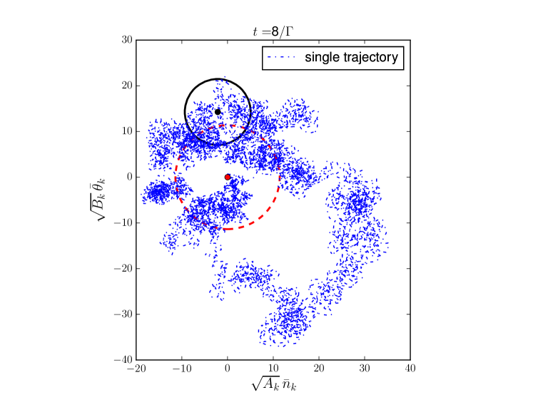
Figure 3: Evolution of the phase-space distribution for a single trajectory from time $t=0$ to $t=8/\Gamma$ in absence of feedback. The mode $k=0.1\sqrt{mg\bar{\rho}}/\hbar$ is considered, with the initial temperature $T_{i}=1.1g\bar{\rho}$ and a loss rate $\Gamma=\omega_{k}/400$. Scattered blue points give the evolution of the center $R$. We verified that $C_{12}$ stays small while, at any time, $A_{k}C_{11}\simeq B_{k}C_{22}\simeq E_{c}/2$, as expected for such a large $\omega_{k}$. The black solid-circle, of radius $\sqrt{E_{C}}$, represents the final RMS width of the Wigner function. For comparison, the red dashed-circle, of radius $\sqrt{E}$, where $E$ is the energy obtained after averaging over 100 trajectories, gives the rms width of the averaged phase space distribution. The coordinates are given in the frame rotating according to the free evolution: namely, the plotted quantity is $\bar{R}=(\bar{n}_{k},\bar{\theta}_{k})=\mathfrak{R}^{-1}(\omega_{k}t){R}$ Note (3).

Averaging over trajectories.

If the loss events are not recorded, then only the quantities averaged over all possible trajectories are meaningful. If the Wigner distribution is initially centered around 0, it will stay centered at 0. Let us investigate its evolution over a time $\Delta t$. For a given quantum trajectory, i.e. a given value $d\xi$, the losses modifies the correlation matrix according to Eq. (15) as well as the center $R$, which acquires the non zero value $R=-d\xi(1-C_{11}/\bar{n};-C_{12}/\bar{n})$. One then has

$$\langle n_{k}^{2}\rangle_{\rm st}(t+\Delta t)=\langle n_{k}^{2}\rangle(t)-\Gamma\Delta t/\bar{n}C_{11}^{2}+d\xi^{2}\left(1-\frac{\langle n_{k}^{2}\rangle}{\bar{n}}\right)^{2}$$ (20)

and

$$\langle\theta_{k}^{2}\rangle_{\rm st}(t+\Delta t)=\langle\theta_{k}^{2}\rangle(t)+\Gamma\Delta t/\bar{n}(1/4-C_{12}^{2})+(d\xi C_{12}/\bar{n})^{2},$$ (21)

where the subscript st specifies this holds for a single trajectory. Averaging over all possible trajectories, we then find, using $\langle d\xi^{2}\rangle_{\rm{tr}}=\Gamma\Delta t\bar{n}$, that losses modify the variances according to

$$\langle n_{k}^{2}\rangle(t+\Delta t)-\langle n_{k}^{2}\rangle(t)=-2\Gamma\Delta t\langle n_{k}^{2}\rangle(t)+\Gamma\Delta t\bar{n}(t).$$ (22)

and

$$\langle\theta_{k}^{2}\rangle(t+\Delta t)-\langle\theta_{k}^{2}\rangle(t)=\Gamma\Delta t/(4\bar{n}).$$ (23)

As expected, Eq. (22) and (23) are equal to those obtained using a master equation description of the loss process Grišins et al. (2016); tobepublished . Due to the diffusive process experienced by $R$, an increased rate in both equations limits the decrease of the mode energy. For phonons, and assuming the loss rate is small compared to the mode frequency, we show in appendix C that the temperature asymptotically goes towards $g\bar{\rho}(t)/2$.

This value of the asymptotic temperature $T_{\infty}$ is particular to the case of an homogeneous gas with a coupling constant evolving according to Eq. (19). For constant $g$ the asymptotic temperature is $T_{\infty}=g\bar{\rho}$ Grišins et al. (2016); tobepublished . For a gas trapped in a harmonic potential we expect $T_{\infty}$ to scale as $g\rho_{p}$, where $\rho_{p}$ is the peak density. The proportionality factor has not been derived yet, but since the averaged density is smaller than $\rho_{p}$, one naively expects that $T_{\infty}$ is smaller than $g\rho_{p}$. Experimentally $T_{\infty}$ has not been identified, while temperatures as low as $0.25\,g\rho_{p}$ have been reported for a harmonically confined gas Rauer et al. (2016).

Using information retrieved from losses detection: quantum feedback.

If the losses are recorded, such that at each time interval $\Delta t$, the values $M_{j}$ are recorded, the trajectory followed by the center of the Wigner distribution, $R$, can be computed exactly, and the heating associated to the diffusion process seen in equations (23) and (22) can be compensated for. One strategy is to perform, during the whole time-evolution, a quantum feedback on the system, based on the knowledge acquired via the atom losses, in order to prevent the center of the Wigner distribution to drift away of the phase space center. Let us here, as an illustration, assumes one is interested in a given mode $k,c$. The most simple back action is to submit the atomic cloud to a potential $V(x)=A(t)\cos(kx)$, where the computed amplitude $A(t)$ depends on the recorded history of the losses. Such a potential could be realized, for instance, using the dipole potential experienced by atoms in laser field. The cosine modulation of the laser intensity can be realized using an optical lattice, or using a spatial light modulator. The contribution to the Hamiltonian of this potential is $\hat{H}_{\rm{fb}}=A(t)\sqrt{N/2}\hat{n}_{k,c}$. In order to counteract the diffusion process of $R$ due to the loss process, one could adjust $A(t)$ such that the feedback Hamiltonian is

$$\hat{H}_{\rm{fb}}=-\hbar\nu\langle\theta_{k,c}\rangle\hat{n}_{k,c}$$ (24)

where, at each time interval, $\langle\theta_{k,c}\rangle$ is computed by integrating the equations of motion including the effect of losses, the free evolution, and the feedback process. This Hamiltonian acts as an active damping, the damping rate $\nu$ preventing $\theta_{k}$ to drift far from the phase space center. The free evolution Hamiltonian, by coupling the two degrees of freedom, will ensure that neither $\theta_{k}$ nor $n_{k}$ drift away. For a large enough damping rate $\nu$, the contribution of $R$ to the energy of the mode is expected to be negligible compared to the contribution of the covariance matrix $C$ and, according to Eq. (18), one expects to reach the ground state. We present numerical results illustrating such a scenario below.

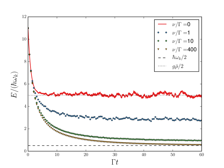
Figure 4: Simulation of the loss process for different feedback strengths $\nu$. Plotted is the time-evolution of the energy in the mode $k$, averaged over 500 quantum trajectories, the parameters being those of Fig. (3). Without feedback the energy converges to $g\bar{\rho}/2$ (horizontal dotted line); lower energies are obtained with feedback and the ground state, of energy $\hbar\omega_{k}/2$ (horizontal dashed line) is reached for large enough $\nu$.

Before presenting numerical results, let us identify the relevant quantities governing the dynamics. Introducing the reduced variable $\tilde{n}_{k}=\bar{n}^{-1/2}n_{k}$ and $\tilde{\theta}_{k}=\bar{n}^{1/2}\theta_{k}$, as shown in appendix D, we find as expected that the cell size $\delta x$ drops out of the problem and, provided time is rescaled by $1/\Gamma$, the dynamics of the mode of wave vector $k$ is solely governed by the dimensionless parameters $\omega_{k}/\Gamma$, $\hbar^{2}k^{2}/(mg\bar{\rho})$ and $\nu/\Gamma$. The relevant measurement signal, for the time interval $\Delta t$, is then $\tilde{M_{k}}=\sqrt{2/N_{at}}\int dxm(x)\cos(kx)$, where $N_{at}$ is the total atom number and $m(x)$ is the number of lost atoms per unit length. Fig. (3), shows the phase-space evolution of a single quantum trajectory, for a mode lying in the phononic regime, in absence of quantum feedback. Fig. (4) shows the time-evolution of the energy in this mode, averaged over quantum trajectories, both in the absence and in the presence of feedback. In the absence of feedback, the energy converges towards the expected value $g\rho/2$. If the feedback scheme is implemented, we observe that the energy in the mode reaches much smaller values. For a large feedback strength $\nu$, the drift of the center is almost completely prohibited and the mode is cooled to its ground state.

Discussion.

In conclusion, we proposed a description of the effect of losses in a many-body system through a Monte Carlo wavefunction approach, and we showed that quantum feedback by monitoring losses could be used to cool down selected modes of a quasi-condensate to vanishing temperatures. This work could be extended in many directions. In view of practical implementation, the sensitivity of the feedback mechanism on the exact knowledge of the system parameters should be investigated. Assuming, as is done in this paper, the system parameters are known exactly, the larger the feedback strength, the better the cooling. In presence of uncertainties, a too large feedback strength will induce heating as it will not match the exact dynamics. Additionally, in most experimental situations the quasi-condensates, trapped in a shallow longitudinal potential, are non homogeneous. Then, the effect of losses depends on the spatial coordinate. Moreover, the linearised description should use, instead of the sinusoidal modes, the spatial density profiles of the Bogoliubov modes, which are not necessarily orthogonal. These issues complicate the picture. Losses might then induce correlations between modes Wade et al. (2015). Another concern is the coupling between modes, which exists beyond the linearized approach considered here. Such coupling is present for instance in the Gross-Pitaevskii equation, which is a classical field approximation of the Lieb-Liniger model. However, long-lived non-thermal states with different Bogoliubov modes experiencing long life-time Langen et al. (2015) have been reported, which indicates small coupling between modes and the possibility to cool down a particular Bogoliubov mode. Finally, note that this cooling process is not limited to 1D systems.

Aknowledgment.

The authors thanks K. Mølmer for inspiring discussions. M. S. gratefully acknowledges support by the German Academic Scholarship Foundation.

Appendix A Effect of losses on the Wigner representation

Here we consider a given mode and we will omit the subscripts $k,r$ to make our notations lighter. We also introduce $\sigma^{2}=\bar{n}/(\Gamma\Delta t)$ and $q_{0}=M_{k}/(\Gamma t)$. Eq. (12) writes, in representation $n$,

$$W(n,\theta)=\frac{1}{\pi}\int du\langle u+n|D|u-n\rangle e^{-2iu\theta}.$$ (25)

The effect of losses, given by Eq (11) transforms the Wigner function of the mode to

$$W^{\prime}(n+M_{k},\theta)=\begin{array}[t]{l}\frac{1}{2\pi^{2}\sigma^{2}}\int du\langle u+n|D|u-n\rangle e^{-2iu\theta}\\ e^{-(n-q_{0}+u)^{2}/(4\sigma^{2})}e^{-(n-q_{0}-u)^{2}/(4\sigma^{2})}.\end{array}$$ (26)

Injecting $\langle u+n|D|u-n\rangle=\int d\tilde{\theta}W(n,\tilde{\theta})e^{i2\tilde{\theta}u}$, we then find Eq. (13).

Let us now consider a Gaussian state. Its Wigner function writes

$$W(n,\theta)=\frac{1}{2\pi\sqrt{det(C)}}e^{-\frac{1}{2}\left[(X-R)^{t}B(X-R)\right]}$$ (27)

where $X=\left(\begin{array}[]{l}n\\ \theta\end{array}\right)$, $R$ is the center of the distribution, $C$ is the covariant matrix and $B=C^{-1}$. The transformation in Eq. (13) transforms the Gaussian state into a new Gaussian state centered on $R^{\prime}$ and of covariance $C^{\prime}$. The convolution on the axis $\theta$ does not change $R$ and changes $C$ in $\tilde{C}$ according to

$$\tilde{C}=C+\left(\begin{array}[]{ll}0&0\\ 0&\frac{1}{4\sigma^{2}}\end{array}\right).$$ (28)

Let us now consider the effect of the multiplication of $W$ by $e^{-\frac{1}{2\sigma^{2}}(n-q_{0}))^{2}}$, as well as the shift along $n$ by $M_{k}$. From Eq. (27), we find

$$B^{\prime}=\left(\begin{array}[]{ll}1/\sigma^{2}&0\\ 0&0\\ \end{array}\right)+\tilde{B}$$ (29)

and

$$\tilde{B}R+\frac{q_{0}}{\sigma^{2}}\left(\begin{array}[]{ll}1\\ 0\end{array}\right)=B^{\prime}\left(R^{\prime}+\left(\begin{array}[]{l}M_{k}\\ 0\end{array}\right)\right)$$ (30)

where $\tilde{B}=\tilde{C}^{-1}$ and $B^{\prime}=C^{\prime-1}$. From Eq. (29), we obtain

$$C^{\prime}=\left(Id+\tilde{C}\left(\begin{array}[]{ll}1/\sigma^{2}&0\\ 0&0\\ \end{array}\right)\right)^{-1}C_{2}$$ (31)

Injecting $\sigma=\sqrt{\bar{n}/(\Gamma\Delta t)}$ and expanding to first order in $\Delta t$, one gets

$$C^{\prime}\simeq\left(Id-\frac{\Gamma\Delta t}{\bar{n}}\left(\begin{array}[]{ll}C_{11}&0\\ C_{12}&0\\ \end{array}\right)\right)\tilde{C}.$$ (32)

Here we used the fact that $\tilde{C}_{11}=C_{11}$ and $\tilde{C}_{12}=C_{12}$. This equation also takes the form of Eq. (15). Let us now consider the center of the distribution. Multiplying the left and right hand parts of Eq. (30) by $C^{\prime}$ and injecting (32), we deduce

$$R^{\prime}=\left(Id-\frac{\Gamma\Delta t}{\bar{n}}\left(\begin{array}[]{ll}C_{11}&0\\ C_{12}&0\end{array}\right)\right)\left(R+\frac{M_{k}}{\bar{n}}\left(\begin{array}[]{l}C_{11}\\ C_{12}\end{array}\right)\right)-\left(\begin{array}[]{l}M_{k}\\ 0\end{array}\right)$$ (33)

Neglecting terms beyond first order in $\Delta t$, we obtain

$$R^{\prime}=R+\left(\frac{M_{k}}{\bar{n}}-\frac{\Gamma\Delta t}{\bar{n}}\langle n_{k}\rangle\right)\left(\begin{array}[]{c}C_{11}\\ C_{12}\\ \end{array}\right)-\left(\begin{array}[]{c}M_{k}\\ 0\\ \end{array}\right).$$ (34)

Injecting $M_{k}=\Gamma\Delta\langle n_{k}\rangle+d\xi$, we recover Eq. (16).

Appendix B Evolution of $E_{C}$ for constant $g$.

We assume $\omega_{k}\gg\Gamma$ such that Eq. (18) is valid. Note that the condition $\omega_{k}\gg\Gamma$ also ensures adiabatic following, namely the time evolution of the Hamiltonian parameters $A_{k}$ and $B_{k}$ preserves the ratio $E_{C}/(\hbar\omega_{k})$, such that Eq. (18) holds both for a constant $g$ and a time-varying $g$. Let us introduce the variable $y=\frac{\langle E_{c}\rangle}{g\bar{\rho}}$ and rewrite Eq. (18) in the form

$$y^{\prime}(t)=y\Gamma\left\{1-\frac{g\rho}{2g\bar{\rho}+\hbar^{2}k^{2}/(2m)}\left(1+y\right)\right\}+\frac{\Gamma\hbar^{2}k^{2}}{8mg\bar{\rho}}.$$ (35)

For $y=1$ we see that $y^{\prime}(t)\geq 0$ and therefore $y(t)$ has to be an increasing function at $y=1$. It follows that for all initial conditions $y(0)\geq 1$ the energy $E_{C}$ stays greater than $g\bar{\rho}$ . This implies in particular that, as long as an excitation stays in the phononic regime (i.e. its frequency stays much smaller than $g\bar{\rho}/\hbar$), it stays in the high temperature regime, namely $E_{C}/(\hbar\omega_{k})\gg 1$.

Appendix C Asymptotic temperature for non-recorded losses

We consider a mode $k$ (we omit the index $r$ for simplicity) and we assume averaging is done over trajectories. Then evolution of the variances of $n_{k}$ and $\theta_{k}$ due to the loss process are given in Eq. (22) and  (23). Let us consider the quantity $\tilde{E}=\langle H_{k}\rangle/(\hbar\omega_{k})$. We assume the loss rate is small enough so that the free evolution under the Hamiltonian (9) ensures equipartition of the energy between the two quadratures, namely at each time $A_{k}\langle n_{k}^{2}\rangle=B_{k}\langle\theta_{k}^{2}\rangle=E/2$. Note that this is equivalent to the condition of adiabatic following. Then the modification of $\tilde{E}$ under the loss process is

$$\frac{1}{\Gamma}\frac{d\tilde{E}}{dt}=-\tilde{E}+(K+1/K)/4$$ (36)

where $K=4\bar{n}A_{k}/\omega_{k}=2\bar{n}\sqrt{A_{k}/B_{k}}$. The evolution under the Hamiltonian (9), provided the adiabatic following condition is satisfied, does not modify $\tilde{E}$. Thus Eq. (36) gives the total time evolution of $\tilde{E}$, and it is valid both when $A_{k}$ and $B_{k}$ depend on time and when they do not depend on time. In this paper, we consider the situation given by Eq. (19), where the exponential decrease of $\bar{\rho}$ is compensated by a time dependence of $g$ such that $K$ is time independent. Then Eq. (36) evolves at long times to

$$\tilde{E}\underset{t\rightarrow\infty}{\rightarrow}(K+1/K)/4.$$ (37)

For phononic modes, for which $k^{2}\ll g\rho$, one has $K\simeq 2\sqrt{g\rho}/k$. Then $\tilde{E}$ goes to $\sqrt{g\rho}/(2k)$ at long times, which gives

$$E\underset{t\rightarrow\infty}{\rightarrow}\frac{1}{2}g\rho.$$ (38)

This energy is very large compared to $\omega_{k}$. Thus the excitation lies in the high temperature limit and its temperature is $T\simeq E\simeq g\rho/2$. Note that, in the case $g$ is constant, then $K$ depends on time and solving Eq. (36) with the time-dependant value of $K$ gives that $E$ converges to $g\bar{\rho}=g\bar{\rho}_{0}e^{-\Gamma t}$, as derived in Grišins et al. (2016).

Appendix D Equations in reduced variables

Here we derive the evolution equations for the reduced variables $\tilde{n}_{k}=n_{0}^{-1/2}n_{k}$ and $\tilde{\theta}_{k}=n_{0}^{1/2}\theta_{k}$. We note $\tilde{R}$ and $\tilde{C}$ the associated mean vector and covariant matrix. Taking into account the exponential decrease of $n_{0}$, Eq. (15) and Eq.(16) give

$$\tilde{C}^{\prime}=\tilde{C}+\Gamma\Delta t\left(\begin{array}[]{cc}-\tilde{C}_{11}^{2}+\tilde{C}_{11}&-\tilde{C}_{11}\tilde{C}_{12}\\ -\tilde{C}_{11}\tilde{C}_{12}&-\tilde{C}_{12}^{2}+\frac{1}{4}-\tilde{C}_{22}\\ \end{array}\right)$$ (39)

and

$$\tilde{R}^{\prime}=\tilde{R}+d\tilde{\xi}\left(\begin{array}[]{c}\tilde{C}_{11}-1\\ \tilde{C}_{12}\\ \end{array}\right)-\frac{1}{2}\left(\begin{array}[]{c}3\Gamma\Delta t\langle\tilde{n}_{k}\rangle\\ -\Gamma\Delta t\langle\tilde{\theta}_{k}\rangle\\ \end{array}\right).$$ (40)

Here $d\tilde{\xi}=\tilde{M}_{k}-\Gamma\Delta t\langle\tilde{n}_{k}\rangle$ where $\tilde{M}_{k}=M_{k}/\sqrt{n_{0}}$. The statistic of trajectory implies that $\tilde{M}_{k}$ follows a Gaussian statistic with $\langle\tilde{M}_{k}\rangle=\Gamma\Delta t\langle\tilde{n}_{k}\rangle$ and $\rm{Var}\tilde{M}_{k}=\Gamma\delta t$.

References

- Grišins et al. (2016) P. Grišins, B. Rauer, T. Langen, J. Schmiedmayer, and I. E. Mazets, Phys. Rev. A 93, 033634 (2016).
- Rauer et al. (2016) B. Rauer, P. Grišins, I. Mazets, T. Schweigler, W. Rohringer, R. Geiger, T. Langen, and J. Schmiedmayer, Phys. Rev. Lett. 116, 030402 (2016).
- Note (0) We express temperature in energy (effectively taking ).
- Saba et al. (2005) M. Saba, T. A. Pasquini, C. Sanner, Y. Shin, W. Ketterle, and D. E. Pritchard, Science 307, 1945 (2005).
- Castin and Dalibard (1997) Y. Castin and J. Dalibard, Phys. Rev. A 55, 4330 (1997).
- Szigeti et al. (2009) S. S. Szigeti, M. R. Hush, A. R. R. Carvalho, and J. J. Hope, Phys. Rev. A 80, 013614 (2009).
- Wade et al. (2015) A. C. Wade, J. F. Sherson, and K. Mølmer, Phys. Rev. Lett. 115, 060401 (2015).
- Vanderbruggen et al. (2013) T. Vanderbruggen, R. Kohlhaas, A. Bertoldi, S. Bernon, A. Aspect, A. Landragin, and P. Bouyer, Phys. Rev. Lett. 110, 210503 (2013).
- Vasilakis et al. (2015) G. Vasilakis, H. Shen, K. Jensen, M. Balabas, D. Salart, B. Chen, and E. S. Polzik, Nat Phys 11, 389 (2015).
- Kuzmich et al. (2000) A. Kuzmich, L. Mandel, and N. P. Bigelow, Phys. Rev. Lett. 85, 1594 (2000).
- Kraft et al. (2007) S. Kraft, A. Günther, J. Fortágh, and C. Zimmermann, Phys. Rev. A 75, 063605 (2007).
- Gericke et al. (2008) T. Gericke, P. Würtz, D. Reitz, T. Langen, and H. Ott, Nat Phys 4, 949 (2008).
- Mora and Castin (2003) C. Mora and Y. Castin, Phys. Rev. A 67, 053615 (2003).
- Note (1) Note that these criteria can be fulfilled within the quasicondensate regime, for a pixel size smaller than the healing length.
- Mølmer and Castin (1996) K. Mølmer and Y. Castin, Quantum Semiclass. Opt. 8, 49 (1996).
- Note (2) .
- Note (3) The free evolution during a time amounts to a rotation in phase space according to the matrix with .
- (18) A Johnson, S Szigeti, M Schemmer, and I Bouchoule. arXiv preprint arXiv:1703.00322, 2017.
- Langen et al. (2015) T. Langen, S. Erne, R. Geiger, B. Rauer, T. Schweigler, M. Kuhnert, W. Rohringer, I. E. Mazets, T. Gasenzer, and J. Schmiedmayer, Science 348, 207 (2015).