Ranking vertices for active module recovery problem

Abstract

Selecting a connected subnetwork enriched in individually important vertices is an approach commonly used in many areas of bioinformatics, including analysis of gene expression data, mutations, metabolomic profiles and others. It can be formulated as a recovery of an active module from which an experimental signal is generated. Commonly, methods for solving this problem result in a single subnetwork that is considered to be a good candidate. However, it is usually useful to consider not one but multiple candidate modules at different significance threshold levels. Therefore, in this paper we suggest to consider a problem of finding a vertex ranking instead of finding a single module. We also propose two algorithms for solving this problem: one that we consider to be optimal but computationally expensive for real-world networks and one that works close to the optimal in practice and is also able to work with big networks.

1 Introduction

Network analysis has many applications in bioinformatics. This includes analysis of co-expression network for gene clustering [8], searching for reporter metabolites for metabolic processes [10], or stratification of tumor samples based on topological distance between somatic mutations in a gene interaction networks [5]. The overall idea is that by taking into account interactions between entities (genes, metabolites, etc.) one can better interpret the corresponding raw data (gene expression, metabolite concentrations, etc.).

One type of network analysis corresponds to the active module recovery problem. The goal of these methods is to find a connected subnetwork (module) that is enriched in individually important vertices. Such module, for example, could correspond to a signalling pathway for protein-protein interaction network [3] or a metabolic pathway for metabolic networks [7].

There are many implementations for active module recovery [6, 3, 1, 11]. These methods share a problem of non-monotonous dependence of the resulting module on the arbitrary significance threshold value. This means that when a method is rerun with a more relaxed threshold not only some vertices can appear, but they can disappear too. This situation is confusing for the user and makes interpretation of the results harder.

In this paper we consider a formulation of the active module problem in terms of connectivity-monotonous vertex ranking. This allows to generated modules for multiple thresholds that are consistent with each other. First, in section 2.1 we formally define the problem and give related definitions. Then, in sections 2.2 and 2.3 we propose two methods to solve the problem: a brute-force-based method and semmi-heuristic method based on solving a series of integer linear programming (ILP) problems. We also define two baseline methods in section 2.4. Finally in section 3 we compare the methods with each other and baseline methods on generated and real networks.

2 Methods

2.1 Formal definitions

In this section we give a formal definition of the active module recovery problem in its ranking variant. Here we consider only networks with a simple structure of an undirected graph.

Let $G=(V,E)$ be a connected undirected graph and $w:V\to[0,1]$ to be a weight function defined on its vertices. There is also an unknown connected subgraph (active module) and corresponding set of vertices $M$. Weights $w$ are assumed to be random variables such that vertices from $M$ are i.i.d. and follow a ”signal” distribution and vertices from $V\setminus M$ are also i.i.d. but follow a ”noise” distribution. Here we consider weights to be corresponding to P-values of a statistical test, where null hypothesis holds for vertices from $V\setminus M$ and corresponding weights follow uniform distribution $U(0,1)$. Following [3] vertices from $M$ are assumed to follow a beta-distribution $B(\alpha,1)$ for some parameter $\alpha$.

Definition 1

Let $G=(V,E)$ be a graph. A vertex ranking of $G$ is a permutation of its vertices $V$. For a ranking $r=(r_{1},r_{2},\ldots,r_{|V|})$ we consider vertices at the beginning of $r$ (e.g. $r_{1},r_{2},\ldots$) to be more important and ranked higher than vertices at the end (e.g. $r_{|V|},r_{|V|-1},\ldots$).

Definition 2

Let us call a vertex ranking $r$ of a connected graph $G$ to be connectivity-monotonous, if all subgraphs $G_{k}$ induced by vertices from ranking prefixes $r_{1..k}=(r_{1},\ldots,r_{k})$ for $k\in{1..|V|}$ are connected.

For convenience we will consider a rank prefix $r_{1..k}$ as a set $\{r_{1},\ldots,r_{k}\}$ rather than a vector if the context requires it.

In this paper we will use AUC (Area Under the Curve) measure to define which ranking $r$ of graph $G$ better recovers module $M$.

Definition 3

AUC value of a vertex ranking $r$ for graph $G=(V,E)$ and module $M\subset V$ can be calculated using formula:

$$AUC(r|M)=\sum_{i=1}^{n}\left(1-\frac{|r_{1..i}\setminus M|}{|V\setminus M|}\right)\frac{[r_{i}\in M]}{|M|},$$

where $[r_{i}\in M]$ is equal to 1 if $r_{i}\in M$ and 0 otherwise.

To summarize we define the considered problem as follows.

Definition 4

Given a connected graph $G$, an unknown active module $M$ and vertices weights $w$ that follow beta- and uniform distributions for vertices from $M$ and $V\setminus M$ correspondingly, the ranking variant of the active module recovery problem consists in finding a connectivity-monotonous ranking $r$ with the maximal value of $AUC(r|M)$.

Later in this paper we consider the parameter $\alpha$ of the beta-distribution $B(\alpha,1)$ to be known. Similarly to [3] one can infer parameters of the beta-uniform mixture from the vertex weights using maximum likelihood approach.

2.2 Optimal-on-average ranking

In this section we describe a method that finds ranking with the maximal expected value of AUC. Correspondingly, we call it optimal-on-average method.

First, let consider a set $D\subset 2^{V}$ of all vertex sets that induce a connected subgraph of $G$ and a discrete probability $P(M)$ defined for all $M\in D$. Together this constitutes a probability space $\mathcal{M}$.

Our task is to find a ranking $r$ with the maximal expected value of AUC score given a vector of vertex weights $w$:

$$E[AUC(r|\mathcal{M})]=\sum_{M\in D}P(M|w)\cdot AUC(r|M).$$ (1)

A conditional probability of a module $P(M|w)$ can be calculated using the Bayes’ theorem:

$$P(M|w)=\frac{P(w|M)\cdot P(M)}{P(w)}\\ =\frac{P(M)}{P(w)}\cdot\prod_{v\in M}B(\alpha,1)(w(v))\cdot\prod_{v\in{V\setminus M}}U(0,1)(w(v)).$$ (2)

Let us rewrite the formula 1:

$$E[AUC(r|\mathcal{M})]=\sum_{M\in D}p(M|w)\sum_{i=1}^{n}\left(1-\frac{|r_{1..i}\setminus M)|}{|V\setminus M|}\right)\frac{[r_{i}\in M]}{|M|}\\ =\sum_{i=1}^{n}\sum_{M\in D}\left(1-\frac{|r_{1..i}\setminus M|}{|V\setminus M|}\right)\cdot\frac{p(M|w)\cdot[r_{i}\in M]}{|M|}.$$ (3)

This allows us to calculate $E[AUC(r|\mathcal{M})]$ iteratively:

$$E[AUC(r_{1..k}|\mathcal{M})]=E(AUC(r_{1..k-1}|\mathcal{M}))+\\ \sum_{M\in D|r_{k}\in M}\left(1-\frac{|r_{1..k}\setminus M|}{|V\setminus M|}\right)\cdot\frac{p(M|w)}{|M|}.$$ (4)

Formula (4) allows to calculate every $r_{1..k}$ prefix ranking only one time.

This can be used to find the best ranking as shown in the algorithm 1. There we fill in an array that for every set of vertices $D[i]$ from $D$ contains a pair of values $dp[i].auc$ – expected AUC value of the best connectivity-monotonous ranking of vertices $D[i]$ and $dp[i].ranking$ – the corresponding ranking. The function $getArea()$ calculates the second summand of formula (4).

Algorithm 1 Optimal-on-average ranking

1:procedure OptimalRanking($V,E$)

2:     $D\leftarrow getConnectedSubgraphs(V,E)$ $\triangleright$ elements of $D$ ordered by size

3:     $dp[D]$ : (auc: Double, ranking: Vector)

4:     for $i=1$ to $|D|$ do

5:         $M\leftarrow D[i]$

6:         for all $v\in M$ do

7:              if $isNotConnected(M\setminus\{v\})$ then

8:                  continue               

9:              $j\leftarrow$ get index of $M\setminus\{v\}$ in $D$

10:              $auc\leftarrow dp[j].auc+getArea(D,dp[j].ranking,v)$

11:              if $auc>dp[i].auc$ then

12:                  $\bar{v}\leftarrow(dp[j].ranking,v)$

13:                  $dp[i]\leftarrow(\bar{v},auc)$                             return $dp[|D|].ranking$

The time complexity of the algorithm 1 is $O(n^{2}\cdot|D|^{2})$. One call to $getArea()$ requires $O(n\cdot|D|)$ time and it is multiplied by $O(n\cdot|D|)$ for the outer loops.

2.3 Semi-heuristic ranking

In this section we describe another approach for the vertex ranking problem. This approach is inspired by BioNet method [3] and consists in solving a series of integer linear programming (ILP) problems using IBM ILOG CPLEX library. Compared to the optimal-on-average approach from the previous section this method allows finding a ranking for large graphs in a rather reasonable time. As this method does not explicitly optimizes AUC score we call this method semi-heuristic.

First, similar to BioNet, let us find a subgraph of $G$ that is most likely to be the active module. The most likely subgraph has the best (log)-likelihood score. The log-likelihood score of the module can be calculated as a sum of log-likelihood scores of the individual vertices in the module, where individual score for vertex $v$ is calculated as:

$$score(v)=\log\mathcal{L}(\alpha,1|w(v))=\log(\alpha\cdot{w(v)}^{\alpha-1}).$$

Now, we can find a connected subgraph $M$ with a maximal sum of vertex scores. This corresponds to an instance of Maximum-Weight Connected Subgraph problem (MWCS). This problem is NP-hard but it can be reduced to an ILP problem and solved by IBM ILOG CPLEX as, for example, in [4].

Using the found subgraph $M$ we can define a crude partial ranking by saying that vertices of $M$ go before $V\setminus M$.

Next, we define a procedure to refine such partial ranking. This procedure takes two sets of vertices: a set $R$ that contains already ranked vertices and a set $C$ that contain set of candidate vertices to be ranked. Then we find a subset $X$ of $C$, so that $R\cup X$ is a connected and vertices from $X$ should be ranked higher than $C\setminus X$.

Using this procedure we can recursively refine ranking up to the individual vertex level. Initially we solve an instance where $R$ is set to an empty set and $C$ contains all vertices. Then we do ranking for $(R,X)$ and $(R\cup X,C\setminus X)$. We stop recursion when the candidate set consists of only one vertex.

A parameter of this procedure is how to select set $X$. For this end, similarly to the first step, we solve an MWCS instance, but with an additional constraint that requires the solution to contain at least one vertex from $R$ and at least one but not all vertices from $C$. We set $X$ as an intersection of the solution and the set $C$. The corresponding instance is solved by a modified solver from [9], where corresponding constraints were added into the ILP formulation.

Overall algorithm is shown as algorithm 2. The procedure $findMaximumSG()$ solves MWCS with the described additional constraints and returns chosen subset of vertices from $C$. If $list$ size is more than one, we call $refineRanking()$ to get a ranking of this set. The algorithm returns a ranking $r$ of vertices $C$.

Algorithm 2 Semi-heuristic ranking refinement

1:procedure refineRanking($V,E,R,C$)

2:     $r$ : Ranking

3:     while $C.size!=0$ do

4:         $list\leftarrow findMaximumSG(V,E,R,C)$

5:         if $list.size>1$ then

6:              $list\leftarrow refineRanking(V,E,R,list)$          

7:         $r.addAll(list)$

8:         $R.addAll(list)$

9:         $C.removeAll(list)$      return $r$

2.4 Baseline methods

As base line for the experiments we consider the following two methods.

The first method ranks vertices by their weights: the smaller the weight, the higher is rank. This ranking is not connectivity-monotonous but is a good starting point. We will call this method non-monotonous.

The second method consists in running BioNet algorithm for ten different significance thresholds. As the BioNet modules ($M_{1}$, $M_{2}$, …, $M_{10}$) can be non-monotonous we use the following combining procedure. We assign the highest rank to vertices from $M_{1}$, the second highest to $M_{2}\ M_{1}$, the third to $M_{3}\setminus(M_{1}\cup M_{2})$ and so on. The significance thresholds are selected to be distributed at equal steps between maximum and minimum log-likelihood vertex scores.

3 Experimental results

We carried three series of experiments for different graph sizes. First, we considered small graphs of about 20 vertices where we were able to thoroughly compare all the considered methods. Next, we analyzed medium-sized graphs of 100 vertices. For such sizes that are closer to the real-world ones we analyzed all methods except optimal-on-average one, as it became computationally infeasible to run. Finally, we tested methods on a real-world graph of two thousand vertices.

3.1 Small graphs

In the first experiment we have generated 32 different graphs of size 18. Then an active module of size 4 was chosen uniformly at random. Value of $\alpha$ was chosen from $U(0,0.5)$ distribution. Vertex weights were generated from corresponding beta- and uniform distributions.

The results of the first experiment are shown on Fig. 1. They show that the optimal-on-average method in most cases works equal or better compared to both BioNet-like and non-monotonous baseline methods (top panels). The semi-heuristic method works similarly well compared to optimal (bottom-left panel) and better than BioNet-like method.

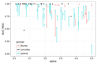
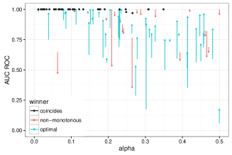
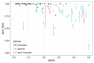
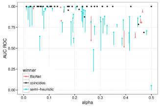
Figure 1: Module AUC values for graphs of size 18. The following methods are present: optimal-on-average, semi-heuristic, BioNet-like and non-monotonous. Each panel shows comparison of two methods. One arrow correspond to one experiment with its ends corresponding to AUC value of the first and the second methods in the pair. The color depends on which method works better. True active modules were sampled from the uniform distribution.

The distribution of active modules can be non-uniform in the real-world data, so we also carried out an experiment with such non-uniform distribution (see 3.4 for details). Aside from the four methods considered before we ran an optimal-on-average method parametrized by the real empirical distribution of the modules.

The results of this experiment are shown on Fig. 2. The situation is similar to the previous experiment with semi-heuristic method being close to optimal-on-average method and better than baseline methods. However, the semi-heuristic method works worse than optimal-on-average method parametrized by the real modules distribution.

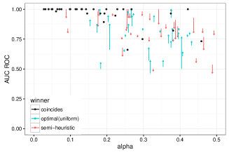
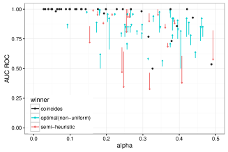
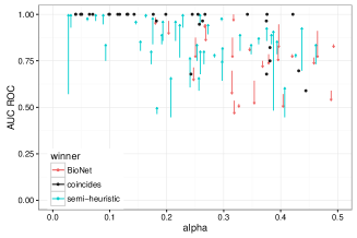
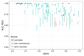
Figure 2: Module AUC values for graphs of size 18 when true active modules were sampled from a non-uniform distribution. The following methods are present: optimal-on-average, optimal-on-average parametrized by the real distribution, semi-heuristic, BioNet-like and non-monotonous.

3.2 Medium-sized graphs

Similarly to the previous section we have generated 32 different graphs of size 100. An active module were sampled to be the size of 5–25.

On these graph sizes running the optimal-on-average method becomes infeasible, so we excluded it from the analysis. A median time of running the semi-heuristic method was 146 seconds.

The results of the experiment are shown on Fig. 3. Almost for all cases semi-heuristic ranking have worked better than both BioNet-like and non-monotonous baseline methods.

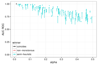
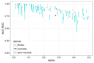
Figure 3: Module AUC values for graphs of size 100. Three methods are present: semi-heuristic, BioNet-like and non-monotonous.

3.3 Large real-world graph

Finally, we analyzed performance of the proposed semi-heuristic method on the large real-word graph. For this experiment we used a protein-protein interaction graph from the example of BioNet package [2]. This graph has 2089 vertices and 7788 edges. An active module in this network was sample to be a size of 50–250.

The results of the experiment are shown on Fig. 4. As for medium sizes semi-heuristic method works better than both baseline methods. On the other hand, the running time of the method increased significantly to about six hours.

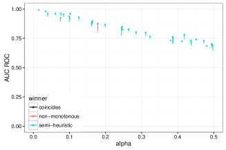
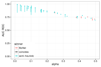
Figure 4: Module AUC values for a real protein-protein interaction graph. Three methods are present: semi-heuristic, BioNet-like and non-monotonous.

3.4 Generating graphs for experiments

To mimic real network graphs generated for the experiments were scale-free. For the generation we used an existing implementation of the Barabasi-Albert algorithm from an R-package igraph.

For subgraph sampling of the given size we used the following procedure. Let $G=(V,E)$ be a connected graph, $k$ be a required size of an active module and $M$ is the set of vertices of the generated random active module. At the beginning $M$ is empty. First we add into $M$ a random vertex from the graph. Next we choose one of the adjacent vertex of $M$ that does not already belong to $M$ and add it. This step is repeated until $M$ is of size $k$.

4 Conclusion

The problem of active module recovery appears in many areas of bioinformatics. Usually it is solved by an heuristic or exact algorithm that provides a module for a selected significance threshold. However, in practice multiple threshold values are tested and the results of these tests are not easily combined to be interpreted. In this paper we considered a ranking variant of this problem, where vertices are ranked before a particular threshold is selected. We also force a property of a module for a more stringent threshold to be a subgraph of a module for a less stringent one. We proposed two methods to solve this problem. The first method uses dynamic programming to find a ranking that maximizes an expected value of AUC score. We consider this method to be optimal, but it works only on small graphs. The second method does not explicitly maximize the AUC score but compares well to the optimal one and works better than the baseline methods in practice. However, it is also able to rank graphs with up to thousands vertices in a reasonable time.

References

- [1] Alcaraz, N., Friedrich, T., Kotzing, T., Krohmer, A., Muller, J., Pauling, J., Baumbach, J.: Efficient key pathway mining: combining networks and OMICS data. Integr Biol (Camb) 4(7), 756–764 (2012)
- [2] Beisser, D., Klau, G.W., Dandekar, T., Muller, T., Dittrich, M.T.: BioNet: an R-Package for the functional analysis of biological networks. Bioinformatics 26(8), 1129–1130 (Apr 2010)
- [3] Dittrich, M.T., Klau, G.W., Rosenwald, A., Dandekar, T., Müller, T.: Identifying functional modules in protein-protein interaction networks: an integrated exact approach. Bioinformatics (Oxford, England) 24(13), i223–31 (2008)
- [4] El-Kebir, M., Klau, G.W.: Solving the maximum-weight connected subgraph problem to optimality (2014), arXiv:1409.5308
- [5] Hofree, M., Shen, J.P., Carter, H., Gross, A., Ideker, T.: Network-based stratification of tumor mutations. Nat. Methods 10(11), 1108–1115 (2013)
- [6] Ideker, T., Ozier, O., Schwikowski, B., Siegel, A.F.: Discovering regulatory and signalling circuits in molecular interaction networks. Bioinformatics (Oxford, England) 18 Suppl 1, S233–S240 (2002)
- [7] Jha, A.K., Huang, S.C., Sergushichev, A., Lampropoulou, V., Ivanova, Y., Loginicheva, E., Chmielewski, K., Stewart, K.M., Ashall, J., Everts, B., Pearce, E.J., Driggers, E.M., Artyomov, M.N.: Network integration of parallel metabolic and transcriptional data reveals metabolic modules that regulate macrophage polarization. Immunity 42(3), 419–430 (2015)
- [8] Langfelder, P., Horvath, S.: Wgcna: an r package for weighted correlation network analysis. BMC Bioinformatics 9(1), 559 (2008)
- [9] Loboda, A.A., Artyomov, M.N., Sergushichev, A.A.: Solving Generalized Maximum-Weight Connected Subgraph Problem for Network Enrichment Analysis, pp. 210–221. Springer International Publishing, Cham (2016)
- [10] Patil, K.R., Nielsen, J.: Uncovering transcriptional regulation of metabolism by using metabolic network topology. Proceedings of the National Academy of Sciences 102(8), 2685–2689 (2005)
- [11] Sergushichev, A.A., Loboda, A.A., Jha, A.K., Vincent, E.E., Driggers, E.M., Jones, R.G., Pearce, E.J., Artyomov, M.N.: GAM: a web-service for integrated transcriptional and metabolic network analysis. Nucleic Acids Res. 44(W1), 194–200 (2016)